
Chapter 35. Connected Component Labeling in CUDA
Ondřej Št´ava and Bedřich Beneš
Connected component labeling (CCL) is a task of detecting connected regions in input data, and it finds its applications in pattern recognition, computer vision, and image processing. We present a new algorithm for connected component labeling in 2-D images implemented in CUDA. We first provide a brief overview of the CCL problem together with existing CPU-oriented algorithms. The rest of the chapter is dedicated to a description of our CUDA CCL method.
35.1. Introduction
The goal of a CCL algorithm is to find a unique label for every set of connected elements in input data. In other words, CCL is used to divide input elements, for example, pixels of a raster image, into groups where all elements from a single group represent a connected object. CCL can be thought of as topological clustering based on connectivity. CCL is often confused with segmentation, which is a closely related algorithm, but its purpose is different. Segmentation is used to detect all elements that describe some object or a feature of interest, whereas CCL is used to identify which of these elements belong to a single
connected
object. An example is a face recognition, where we can first use segmentation to detect all pixels that correspond to a human eye and then we can apply CCL to find a single group of pixels for every eye in the image. Another example of CCL is in
Figure 35.1
.
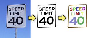 |
| Figure 35.1
Connected component labeling as a part of a text recognition pipeline. The input image (left) is segmented, and all pixels that might represent a text are retrieved (middle). Connected component labeling is then used to separate pixels into groups that represent individual characters (right). Each detected group is depicted with a different color.
|
The CCL problem is usually solved on the CPU using sequential algorithms
[1]
, but the speed of these algorithms is often not sufficient for real-time applications. Certain CCL algorithms can be parallelized, but as has been pointed out in
[2]
, the sequential algorithms often outperform the parallel ones in real applications.
We propose a new parallel algorithm for CCL of 2-D data implemented in CUDA. The input is a 2-D grid of values where each value represents a unique segment in the input data. The output is a new 2-D array where all connected elements with the same segment value share the same label. Our implementation detects connected components with Moore neighborhood (8-degree connectivity)
[3]
and the method can be easily extended for N-dimensional grids and different connectivity conditions.
The CCL problem has been a research topic for a long time, and algorithms that provide a solution in linear time have been presented
[1]
. Most of these CPU-oriented algorithms are sequential in nature, and they usually require multiple passes over the input data. The most commonly used algorithms use two passes where the first pass detects and stores equivalences between all connected neighboring elements, and the second pass analyzes the equivalences and assigns labels to individual elements. The equivalences between elements are usually stored in a disjoint set forest data structure that contains several equivalence trees where each tree represents a single connected component (see
Figure 35.2
). In these two pass algorithms, it is necessary to find an equivalence tree for every connected component of the input data in the first pass, as in the second pass the equivalence trees are used to assign labels to the input elements. To compute all equivalence trees in one pass, it is necessary to traverse the data in a fixed order and to gradually update the equivalence trees for each processed element. The most widely used method that is used to for this task is the
union-find
algorithm that ensures that the equivalence trees are always correct for all processed elements
[1]
.
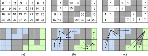 |
| Figure 35.2
Equivalence trees representing two connected components. All equivalences are stored in a 2-D array where every element is identified by its address in the array (a). All elements from one equivalence tree represent a single connected component (b). To get the final labels of the components, the equivalence trees are simply flattened (c).
|
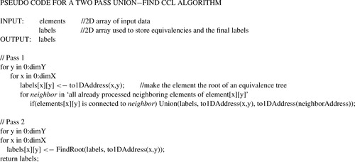
A pseudo code for a simplified version of a two-pass
union-find
CCL algorithm for 2-D raster data is described in
Figure 35.3
. Here, the equivalence trees are stored in a 2-D array with the same dimensions as the input data. All elements are identified by their 1-D address so that the root of an equivalence tree is the element with the entry in the equivalence array equal to the address of the element itself. The elements are processed in a scan-like fashion, and every analyzed element updates the equivalence array from its connections with other already-processed neighboring elements using the
Union
function (see
Figure 35.4
). In the second pass, all equivalence trees are flattened using the
FindRoot
function. After the flattening, each element is equivalent directly to the root of the tree (see
Figure 35.2c
) and the value of the root (address of the root element) is used as the label for the detected connected component. The labels generated by this algorithm are not consecutive because they are based on the address of the root element, but they can be easily relabeled.
 |
| Figure 35.3
Pseudo code for a two pass union-find CCL algorithm.
|
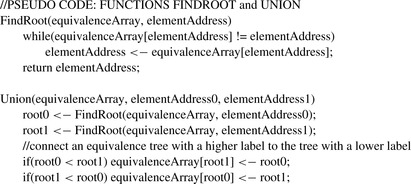 |
| Figure 35.4
Pseudo code for functions
FindRoot
and
Union
.
|
35.2.1. Parallel Union Find CCL Algorithm
The algorithm from
Figure 35.3
can be implemented on many-core devices such as GPUs. Hawick
et al
.
[2]
implemented the union-find CCL algorithm using three CUDA kernels. They demonstrated that
their implementation provides a significant performance gain over an optimized CPU version for most of the tested data. The main drawback of the parallel two-pass CCL algorithms is that it is impossible to guarantee that a single equivalence tree is constructed for a single connected component of the input data in the first pass of the algorithm. The problem is that the equivalences of all elements are processed in parallel, and therefore, it is difficult to merge the new equivalences with the results from previously
processed elements using the
Union
function. In many cases, the first pass of the algorithm will generate multiple disjoint equivalence trees for a single connected component of the input data, and to merge the trees into a single one, it is necessary to iterate several times. The exact number of the iterations is unknown because it depends on the structure of the connected components in the input data. Therefore, it is necessary to check after each iteration whether all connected elements have the correct labels. In the case of a CUDA algorithm, it is necessary to perform the check on the GPU and to upload the result back to the host, which can then execute another iteration of the kernels. Also, when the union-find CCL algorithm is directly mapped to CUDA, it is problematic to take advantage of the shared memory on the GPU because one kernel is used to compute equivalencies between all input data elements, and the resulting equivalence trees are too large for the shared memory of existing GPUs.
35.3. CUDA Algorithm and Implementation
We present a new version the two-pass union-find algorithm where all iterations are implemented inside the kernels. The number of the executed kernels is fixed for a given dimension of the input data, and no synchronization between the host and device is needed. Our method also takes advantage of shared memory on the GPU as we divide the input data into smaller tiles where the CCL problem is solved locally. The tiles are then recursively merged using a treelike hierarchical merging scheme as illustrated in
Figure 35.5
. At each level of the merging scheme, we use border regions of neighboring tiles to merge the local solution of the CCL problem from lower levels.
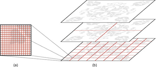 |
| Figure 35.5
Two main steps of our algorithm. First, the CCL problem is solved locally for a small sub-set of input data in shared memory (a). The global solution is then computed by a recursive merging of the local solutions (b).
|
All of the steps of our algorithm are implemented entirely on the GPU in four different kernels (see
Figure 35.6
. Kernel 1 solves the CCL problem for small tiles of the input data in shared memory. Then, the merging scheme is recursively applied on the border regions between the tiles. The merging scheme uses two different kernels. One merges together equivalence trees from a set of tiles, and the second one updates labels on border regions of the data tiles before each iteration of the merging scheme. The merging scheme is used only to merge equivalence trees from connected tiles; therefore, when all tiles on all levels are merged, it is necessary to find the final solution of the CCL problem by updating labels
on all data elements. This process is done in the last kernel. Both the first kernel and the final kernel are called only once, while the merging scheme kernels are called for each level of the merging scheme. The number of levels is determined by the dimensions of the input data; therefore, it does not depend on the structure of the connected components in the analyzed data. This is a great advantage of our algorithm because it reduces the number of executed kernels, and it also eliminates all data transfer from the device to the host. Although the number of kernel calls is fixed for given dimensions of input data, it is still necessary to execute a different number of iterations of our CCL solver even if they have the same dimensions. However, all these iterations are performed directly inside the kernels 1 and 2, and they are effectively hidden from the host. The kernels are described in detail in the next sections.
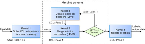 |
| Figure 35.6
A flowchart of our CUDA CCL algorithm.
|
The CCL algorithm is written in CUDA 3.0 and C++, and all source code is available in an attached demo application. The CCL algorithm requires a GPU with computing capability 1.3 or higher because the kernels use atomic operations both on global and shared memory. The demo application also requires CUDA Toolkit 3.0 because it exploits the OpenGL interoperability functions introduced in this release.
35.3.2. Input and Output
The connectivity criterion must be first explicitly defined by the user, and it is one of the parameters of our algorithm. For example, we can say that two elements of an RGB image are connected if the difference between their luminance is below a given threshold value. Another way to define the connectivity criterion is to apply segmentation
[5]
and
[6]
on the input data. In segmented data, two neighboring elements are connected only when they share the same segment value, and this is also the approach we chose in our implementation. The input data are stored in a 2-D array of 8-bit unsigned integers that contain the segment values for all elements with the exception of the segment value 0 that denotes the background and is ignored by our CCL algorithm.
The connected components are then detected for every nonbackground element using segment values from the Moore neighborhood. All connected components are represented by labels that are stored in a 32-bit integer 2-D array that has the same dimension as the input data. The same array stores the equivalence trees as described in
Section 35.2
.
35.3.3. CCL in Shared Memory
Kernel 1 finds first the local solution of the CCL problem for a small tile of the input data in the shared memory of the GPU (see the pseudo code for the kernel in
Figure 35.8
). Each tile is solved by one CUDA thread block, and each thread corresponds to a single element in the given tile. The local solution is obtained from a modified version of the two-pass CCL solver that has been described in
Figure 35.3
. The kernel executes a new iteration of the modified CCL algorithm whenever any two neighboring connected elements have a different label. Each iteration performs both passes of the algorithm, but the first pass is divided into two separate steps. First, each thread detects the lowest label from all neighboring elements. If the label from neighboring elements is lower than the label of the processed element (two connected elements belong to different equivalence trees), then we merge these equivalence trees using the
atomicMin
function. The atomic operation is necessary because the same equivalence tree could be updated by multiple threads at the same time. This CCL algorithm is demonstrated in a simple example in
Figure 35.7
. The final labels are related to the address space of the shared memory because it provides an easier addressing pattern for the memory access. Therefore, after all iterations complete, it is necessary to transfer the labels into the global address space and then store them in the global device memory.
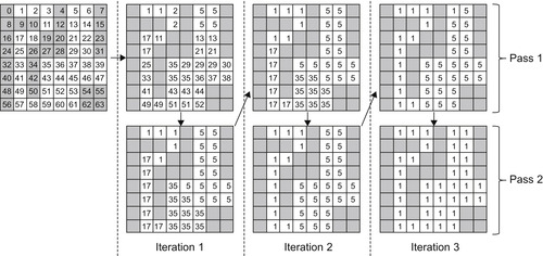 |
| Figure 35.7
Application of the modified CCL algorithm for kernel 1 on a simple example.
|
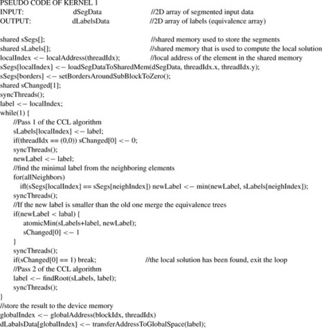 |
| Figure 35.8
Pseudo code of kernel 1.
|
35.3.4. Merging Scheme
To compute a global solution of the CCL problem, it is necessary to merge the local solutions from the previous step. We can use the connectivity between all border elements of the two tiles to merge the equivalence trees of the connected components in respective tiles. Because we want a parallel solution of the problem, it is usually necessary to perform several iterations of this merging operation
because we cannot guarantee that all equivalence trees are merged after a single merge operation. This iterative mechanism needs synchronization between individual threads of a single thread block, but in general, it is not feasible to process all border elements in one thread block because there are neither enough threads, nor enough shared memory to store all the required data. Our solution of this problem is implemented in kernel 2 and illustrated in
Figure 35.9
. A given set of tiles is merged in one 3-D thread block where the x and y dimensions of the block are used to index individual tiles while the z dimension contains individual threads that are used to compare and merge equivalence trees on a given tile boundary using the
Union
function. Because the number of threads associated to each tile is not large enough to process all boundary elements of a given tile, all threads actually process multiple boundary elements sequentially. In the first stage, the threads process elements on both sides of the bottom horizontal boundary, and in the second stage, they process both sides of the right vertical boundary. If the boundary between two tiles is too long, the thread processes one boundary sequentially before proceeding to the next one. As we can see in
Figure 35.9
, the corner elements between four tiles are processed by multiple threads, but the number of these redundant threads is low and does not require special treatment.
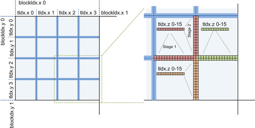 |
| Figure 35.9
Left: One CUDA thread block is used to merge 16 tiles that contain local solutions to the CCL problem from previous steps of our algorithm. Right: Threads in the CUDA block are used multiple times to process different boundaries of the merged tiles.
|
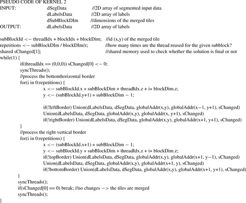
One execution of kernel 2 can merge only a limited number of tiles together, so it is necessary to call the kernel multiple times where each iteration of the kernel takes the merged tiles from previous steps as an input. The number of tiles that are merged in each level can vary. We found out that merging 4 × 4 tiles produces good results. If we merge more tiles on one level, then the number of threads associated with each tile is too small, and the whole process becomes more sequential. On the other hand, if we merge fewer tiles, then the number of levels of the merging scheme increases — a result that is also not desirable. Pseudo code for kernel 2 is given in
Figure 35.10
. Connected component (equivalence trees) from neighboring tiles are merged using the
Union
function. The implementation of the
Union
functions follows the description from
Figure 35.4
in
Section 35.2
. However, multiple threads might try to merge two equivalence trees at the same time, and that is why the merging operation is implemented using the
CUDA
atomicMin
function. When two connected elements are located in different equivalence trees (trees that have a different root label), we set the shared variable
sChanged
to 1, which indicates that another iteration of the algorithm is necessary.
 |
| Figure 35.10
Pseudo code of kernel 2.
|
It is important to mention that the output from kernel 2 is not a complete solution of the CCL problem for the given tiles because it only merges different equivalence trees together, but the labels on nonroot elements remain unchanged. However, it is guaranteed that each equivalence tree in the merged tile represents the largest possible connected component. The advantage of this approach is that the labels are updated only on a relatively small number of elements, and the amount of data written to global memory is usually small. The drawback is that as we merge more and more tiles together, the depth of equivalence trees on the border elements of the merged tiles may increase significantly, making
the
Union
operation slower. To solve this problem we use kernel 3 to flatten the equivalence trees on border elements between tiles using the
FindRoot
operation (see
Figure 35.4
). The kernel is always executed between two consecutive kernel 2 calls as illustrated in
Figure 35.6
. Although our method would work even without kernel 3, the observed performance gain from using it is around 15–20%.
35.3.5. Final Update
When all tiles are merged, we can compute the global solution of the CCL problem. The labels in the final merged tile represent a disjoint equivalence forest where it is guaranteed that every tree corresponds to the largest possible connected component. To obtain the final solution, we flatten each equivalence tree using the
FindRoot
function that is called from kernel 4 for every element of the input data.
35.4. Final Evaluation and Results
To evaluate the performance of our method, we measured throughput of our implementation and speedup over other CCL algorithms. Namely, we implemented an optimized CPU CCL algorithm described by Wu
et al
. in
[1]
and a CUDA-oriented algorithm by Hawick
et al
. in
[2]
. Because the input data were represented by 8-bit integers and output data by 32-bit integers, we decided to measure the throughput in megapixels per second where each pixel represented a single element in the input dataset. All measurements were performed on the same computer with 64-bit Windows 7, 3 GHz Intel
Core 2 Duo CPU, and NVIDIA GeForce GTX 480 GPU. We didn't measure transfers of the input and output data between the host and the device as these operations are application dependent.
The complexity of a CCL problem depends on the structure of the connected components in the input data and the performance of each method can differ dramatically for different datasets. Hence, to perform an unbiased analysis, CCL algorithms should be tested on a variety of different input cases. There is no standardized set of input data designed for the performance testing, and therefore, we created several test cases that, in our opinion, represented common real-world scenarios. Results of all of our measurements are summarized in
Figure 35.11
.
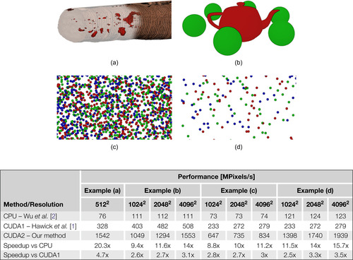 |
| Figure 35.11 |
First, we applied all tested algorithms in real-world settings in our application for defect detection in 3-D CT data of a wooden log (Figure 35.11a
). The algorithm was used to detect potential defect regions in hundreds of main-axis parallel 2-D slices with resolution of 512 × 512 pixels. The second example (Figure 35.11b
) is a scene with a small number of large objects that filled most of the analyzed data
space. The example was tested for different resolutions of input data, while the scene was rescaled to fit the dimensions of the data. For the final two examples, we generated a high number of small objects that were randomly scattered in the data space. Both cases were analyzed for different resolutions of input data, but in this case, we kept the scale of the objects locked and repeated the same pattern on a larger canvas. In the first case (Figure 35.11c
) the base resolution (1024 × 1024) contained 2500 spheres that filled almost the entire canvas, whereas in the second case (Figure 35.11d
), we generated only a sparse set of 250 spheres for the base resolution.
Results of all tested algorithms for all examples are summarized in the table in
Figure 35.11
. We can see that the speedup of our algorithm was about 10–15x compared with the tested CPU algorithm and on average about 3x compared with the Hawick's CUDA algorithm. We can also see that our algorithm performs best when the distribution of connected components in the analyzed data is sparse, as shown in Examples 1 (Figure 35.11a
) and 4 (Figure 35.11d
). On the other hand, the speedup is not so high when the connected components cover most of the input data (Figure 35.11b, c
). If we compare results measured on different resolutions of a single experiment, we can observe that our algorithm had the best scalability of all three tested methods because the measured throughput [M pixels/s] increased significantly when we increased the resolution of the data. In the case of the CPU algorithm and the Hawick's CUDA algorithm, the throughput usually remained unaffected by the resolution.
35.4.1. Performance Analysis of Kernels
To further study the performance of our method, we also measured the relative time spent on individual kernels for examples from the previous section (see
Figure 35.12
). We can observe that for all tested examples, the most time-consuming kernels are kernels 1 and 2 that are used to compute the equivalence trees for individual connected components. The only purpose of kernels 3 and 4 is to flatten the equivalence trees (a relatively simple operation), and therefore, their contribution to the final computational time is rather small. Another interesting observation is that the relative time spent on merging of the equivalence trees from different tiles (kernel 2) decreases as the dimensions of the input data increases, thereby showing the effectiveness of our merging scheme.
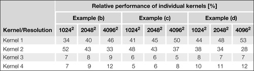 |
| Figure 35.12
Relative work distribution among individual kernels for different examples from
Figure 35.11
.
|
35.4.2. Limitations
One drawback of our method is that it does not generate consecutive final labels because each label has a value of some element from a given connected component. In order to obtain consecutive labeling,
we can apply the parallel prefix sum algorithm
[7]
on the roots of all detected equivalence trees, or we can reindex the labels on the CPU. Another limiting factor is that our implementation works only with arrays that have a size of power of two in both dimensions.
35.4.3. Future Directions
The current implementation of our CCL method provides a solid performance that is sufficient for most common cases, but still, some applications might be more demanding. A feasible solution for these cases would be to solve the CCL problem on multiple GPUs. To add support of multiple GPUs to our method, it would be necessary to modify the merging scheme by including an additional merging step that would be used to merge local solutions from different devices.
To increase the performance of our method itself, it might be interesting to explore possible optimizations of kernels 1 and 2. In the current implementation kernel 1 uses one CUDA thread to process one element, but it might be more optimal to use one thread for multiple elements because in that case we could take advantage of many optimizations proposed for sequential CCL algorithms
[1]
. The performance of kernel 2 could be potentially improved by using shared memory to speed up comparison of the equivalence trees on the boundaries of merged tiles.
References
[1]
K. Wu, E. Otto, K. Suzuki,
Optmizing two-pass connected-component labeling algorithms
,
Pattern Anal. Appli.
12
(2009
)
117
–
135
.
[2]
K.A. Hawick, A. Leist, D.P. Playne,
Parallel Graph Component Labelling with GPUs and CUDA
,
Parallel Comput.
36
(2010
)
655
–
678
.
[3]
L. Gray,
A Mathematician looks at Wolfram's new kind of science
,
Not. Am. Math. Soc.
50
(2003
)
200
–
211
.
[4]
K. Suzuki, I. Horiba, N. Sugie,
Fast connected-component labeling based on sequential local operations in the course of forward raster scan followed by backward raster scan
,
In:
Proceedings of the 15th International Conference on Pattern Recognition (ICPR'00)
,
vol. 2
(2000
)
IEEE Computer Society
,
Los Alamitos
, pp.
434
–
437
.
[5]
R.M. Haralick, L.G. Tarjan,
Image segmentation techniques
,
Comput. Vis. Graph. Image Process
29
(1
) (1985
)
100
–
132
.
[6]
J. Shi, J. Tarjan,
Normalized cuts and image segmentation
,
IEEE Trans. Pattern Anal. Mach. Intell.
22
(8
) (2000
)
888
–
905
.
[7]
M. Harris, S. Sengupta, J.D. Owens,
parallel prefix sum (scan) with CUDA
,
In: (Editors: M. Pharr, R. Fernando)
GPU Gems 3
(2007
)
Addison Wesley
;
pp. 851–576
.
..................Content has been hidden....................
You can't read the all page of ebook, please click here login for view all page.