
Chapter 44. Using GPUs to Accelerate Advanced MRI Reconstruction with Field Inhomogeneity Compensation
Yue Zhuo, Xiao-Long Wu, Justin P. Haldar, Thibault Marin, Wen-mei W. Hwu, Zhi-Pei Liang and Bradley P. Sutton
Magnetic resonance imaging (MRI) is a flexible diagnostic tool, providing image contrast relating to the structure, function, and biochemistry of virtually every system in the body. However, the technique is generally slow and has low sensitivity, which limits its application in the clinical environment. Several significant advances in the past 10 years have created potential solutions to these problems, greatly increasing imaging speed and combining information from several acquisitions to increase sensitivity. But the computational time required for these new techniques has limited their use to research settings. In the clinic, images are needed at the conclusion of a scan to immediately decide if a subject moved, if the correct location was imaged, or if sufficient signal and contrast were obtained. Therefore, to achieve clinical relevance, it is necessary to accelerate the advanced MRI image reconstruction techniques.
In this chapter, we focus on a GPU implementation for a fast advanced non-Cartesian MRI reconstruction algorithm with field inhomogeneity compensation. The parallel structure of the reconstruction algorithms makes it suitable for parallel programming on GPUs. Accelerating this kind of algorithm can allow for more accurate image reconstruction while keeping computation times short enough for clinical use.
44.1. Introduction
MRI is a relatively new medical imaging modality developed by Professor Paul Lauterbur in the early 1970s, for which he was awarded a Nobel Prize in 2003. MRI can be used to measure the structure and function of tissue inside of living subjects, such as human brain tissue, by manipulating the magnetization of nuclei (typically hydrogen nuclei in water) placed in a highmagnetic field. MRI is a noninvasive technique that can be manipulated to obtain different types of image contrast. Nowadays, MRI has become a mature medical imaging technology with many different clinical applications, for example, functional neuroimaging of the brain and cardiovascular imaging.
However, several challenges exist that limit the application of MRI in the clinical environment. Traditionally, the main limitations in MRI have been due to the manner in which data are sampled in clinical scans. Clinical data have been sampled in a Cartesian (i.e., rectilinear) manner to facilitate image reconstruction through the use of the fast Fourier transform (FFT). Cartesian sampling can place a significant limit on acquisition speed. In addition, image artifacts can also exist in MRI owing to susceptibility-induced magnetic field inhomogeneity. Accurate spatial localization in MRI relies on having a uniform magnetic field across the region of the patient's anatomy that is being imaged. Disruptions to this uniformity (called magnetic field inhomogeneity) can cause artifacts in reconstructed images, such as spatial distortions and signal loss. Because good acquisition efficiency and image quality have always been important objectives in MRI, advanced reconstruction techniques that can accommodate non-Cartesian data acquisition and field inhomogeneity have also become critical issues.
In this chapter, we introduce an MR imaging toolbox that implements a fast reconstruction algorithm using parallel programming on GPUs. This chapter is designed to assist researchers working in medical imaging and reconstruction algorithm development, especially in the area of MR image reconstruction. Many advanced acquisition and reconstruction strategies exist in research environments, but their implementation in the clinic has been impeded by their large computational requirements. Thus, this chapter describes a platform for the translation of these advanced schemes to the clinic by enabling clinically-relevant computational times. Furthermore, the speedup of image reconstruction will significantly influence the application and future development of imaging in a variety of application areas (e.g., functional brain imaging of depression and memory, detection of cancer, and evaluation of heart disease). The rest of this chapter is organized as follows: First, we describe recent technologies in MRI that are easily ported to the GPU to enable clinically useful computational times. Second, the implementation of the advanced MRI reconstruction algorithm on GPUs is presented. Finally, we will provide the implementation results and an evaluation on a sample acquisition of a brain slice for functional imaging.
44.2. Core Method: Advanced Image Reconstruction Toolbox for MRI
44.2.1. Non-Cartesian Sampling Trajectory
Traditional MRI data acquisition can be viewed as sampling information in the spatial frequency domain (k-space), and images can be reconstructed using the Fourier transform (FT). For Cartesian trajectories (Figure 44.1(a)
), image reconstruction can be performed using the fast Fourier transform (FFT) algorithm. Using the FFT can reduce the computational complexity from
O
(N
2
) to
O
(N
⋅ log(N
)) for two-dimensional images, where
N
is the total number of pixels in the final reconstructed image. Although the FFT is an efficient reconstruction method, additional techniques are required for the reconstruction of data sampled on non-Cartesian sampling trajectories. Non-Cartesian sampling trajectories (e.g., the spiral trajectory) might be preferable in some situations because they can offer more efficient coverage of k-space (Figure 44.1(b)
) and shorter acquisition times, and provide additional opportunities for balancing the spatial and temporal resolution in data acquisition. To maintain some of the speed advantage of the FFT, the gridding method for non-Cartesian reconstruction
[11]
allows for interpolation of non-Cartesian data onto a Cartesian grid. However, this method suffers from inaccuracies introduced by interpolation. In addition, gridding methods that use the FFT in reconstruction do not inherently allow for the modeling of additional physical effects during the data acquisition process. Thus, gridding can lead to image artifacts, including geometric distortions and signal loss. Compensating for physical effects such as magnetic field inhomogeneity in the gridding reconstruction requires further approximations and interpolations. Recently introduced inverse-problem approaches to image reconstruction formulate a physical model that can incorporate additional physical effects in order to correct images and reduce distortion.
 |
| Figure 44.1
Cartesian and non-Cartesian MRI sampling trajectories in k-space.
|
44.2.2. Susceptibility-Induced Magnetic Field Inhomogeneity Compensation
In MRI reconstruction, advanced imaging models can correct for geometric distortion and some of the signal loss that is due to susceptibility-induced magnetic field inhomogeneity. Field inhomogeneity is due to the fact that air and tissue in the human brain have very different magnetic susceptibilities, which leads to large deviations in the local magnetic field. The susceptibility-induced magnetic field inhomogeneity near the interface of air/tissue (e.g., in the orbitofrontal cortex) can cause geometric distortions and signal loss in reconstructed images as reported in
[12]
[15]
[16]
and
[18]
. As illustrated in
Figure 44.2
, signal loss results from susceptibility-induced magnetic field inhomogeneity gradients (called susceptibility gradients), which cause dephasing of the signal within a voxel. Methods exist for compensating for these susceptibility artifacts. Noniterative, Fourier-transform-based correction methods cannot compensate for signal loss, but only for geometric distortion. Statistical estimation (using a physical model including the effects of susceptibility gradients on the received signal) is a natural alternative, and reconstructions can be obtained in this framework using iterative algorithms.
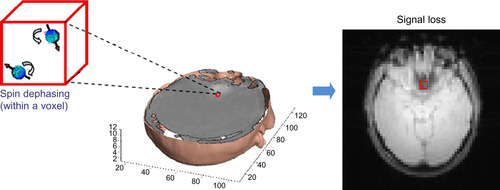 |
| Figure 44.2
Signal loss (one kind of susceptibility-induced field inhomogeneity artifact) caused by spin dephasing within a voxel.
|
Our previous work builds a physical model that accounts for field inhomogeneity and both the within-plane and through-plane susceptibility gradients to correct for geometric distortions and signal loss
[21]
and
[22]
, as shown in
Eq. 44.1
.
 where
d
denotes the complex k-space signal; ρ(r
) is the object at location
r
;
k
(t
m
) is the k-space sampling trajectory (which can include the Z-shimming imaging gradient
[9]
) at time
t
m
; and ω(r
) = ω(x
,
y
,
z
) represents the magnetic field inhomogeneity map (including the susceptibility gradients in X, Y, Z directions), which can be parameterized in terms of 3-D rectangle basis functions as in
Eq. 44.2
.
where
d
denotes the complex k-space signal; ρ(r
) is the object at location
r
;
k
(t
m
) is the k-space sampling trajectory (which can include the Z-shimming imaging gradient
[9]
) at time
t
m
; and ω(r
) = ω(x
,
y
,
z
) represents the magnetic field inhomogeneity map (including the susceptibility gradients in X, Y, Z directions), which can be parameterized in terms of 3-D rectangle basis functions as in
Eq. 44.2
.
 N
is the number of spatial image voxels; ω
n
is off-resonance frequency for each voxel (in Hz);
G
x,n
,
G
y,n
are the within-plane susceptibility gradients and
G
z,n
is the through-plane susceptibility gradient (in Hz/cm); φ
n
(x
,
y
,
z
) represents the basis function; and (x
n
,
y
n
,
z
n
) denotes the location of the center of the
n
th voxel. Using this model, geometric distortion and signal loss induced by both within-plane and through-plane susceptibility gradients
[21]
and
[22]
can be compensated simultaneously.
N
is the number of spatial image voxels; ω
n
is off-resonance frequency for each voxel (in Hz);
G
x,n
,
G
y,n
are the within-plane susceptibility gradients and
G
z,n
is the through-plane susceptibility gradient (in Hz/cm); φ
n
(x
,
y
,
z
) represents the basis function; and (x
n
,
y
n
,
z
n
) denotes the location of the center of the
n
th voxel. Using this model, geometric distortion and signal loss induced by both within-plane and through-plane susceptibility gradients
[21]
and
[22]
can be compensated simultaneously.
(44.1)
(44.2)
44.2.3. Advanced MR Imaging Reconstruction Using Parallel Programming on GPU
The motivation of this work is to reduce computation time by implementing our advanced MRI reconstruction method (that compensates for magnetic field inhomogeneity and accommodates non-Cartesian sampling trajectories) using parallel programming with CUDA on GPUs. On a typical CPU, the iterative reconstruction method requires long computation times that are not tolerable for clinical applications. Fortunately, the iterative MRI reconstruction framework can greatly benefit from a fast GPU-based implementation. Our implementation used techniques to optimize the memory management and computation, including use of constant memory with tiling, and use of fast hardware math functions. These and several other optimization techniques will be discussed in
Section 44.3.2
. Our implementation makes use of the iterative conjugate gradient algorithm
[6]
for matrix inversion. Our implementation also includes a regularization term that can contain prior information (we use a spatial smoothness constraint in our implementation using the prior knowledge that MR images are typically smooth). The computation related to this regularization term was implemented on the GPUs using sparse matrices (see
Section 44.3.2
). In contrast to our previous work that implemented regularized image reconstruction without field inhomogeneity compensation
[19]
, we have currently implemented the entire conjugate gradient algorithm on the GPU to avoid time-consuming data transfers between the CPU and the GPU. Finally, we have developed a MATLAB toolbox to facilitate the access to the GPU reconstruction algorithm, and to visualize the reconstructed images (see
Section 44.3.3
). This toolbox was designed to enhance the accessibility of the distributed version of the GPU implementation. We will show that our implementation on GPUs achieved a significant speedup with clinically viable reconstruction times.
44.3. MRI Reconstruction Algorithms and Implementation on GPUs
In this section, we first introduce the algorithms used for the advanced MRI reconstruction. Then we present the details of the fast implementation of the algorithm on GPUs using CUDA-based parallel programming.
44.3.1. Algorithms: Iterative Conjugate Gradients
The implementation of the iterative conjugate gradient (CG) algorithm used in this work is based on
[21]
and solves the optimization problem shown in
Eq. 44.3
:
 where
G
(also called the forward operator) is the system matrix modeling the MR imaging process (including non-Cartesian sampling and a model for the effects of field inhomogeneity),
R
is a penalty functional that encourages spatially smooth reconstructions, and β is a weighting factor. In our imaging model,
G
includes the zero order (causing geometric distortion) and first order (causing signal loss) effects of magnetic field inhomogeneity. These terms modify the relationship between
d
and
ρ
so that a direct FFT is not a good approximation of
G
even when data is sampled with a Cartesian trajectory. The process of directly calculating and storing
G
leads to storage problems with large datasets and long computation times. Moreover, because the FFT cannot be used (without additional approximations and algorithmic complexity
[7]
), reconstruction cannot benefit from the GPU implementations of the FFT in the CUDA library. Thus, one key point of this work is to solve the problem of calculating the system matrix
G
in a reasonable amount of time while keeping storage requirements within the constraints imposed by the GPU. Our solution for limiting memory usage is to compute the entries of
G
as they are used during matrix-vector multiplications and to store the final results of matrix-vector multiplication rather than the full
G
matrix. Similarly, in implementation of the CG algorithm (see
Table 44.1
), we also only store the entries of
G
H
d
instead of
G
H
for each voxel (the so-called backward operator), where
H
denotes the complex conjugate transpose.
where
G
(also called the forward operator) is the system matrix modeling the MR imaging process (including non-Cartesian sampling and a model for the effects of field inhomogeneity),
R
is a penalty functional that encourages spatially smooth reconstructions, and β is a weighting factor. In our imaging model,
G
includes the zero order (causing geometric distortion) and first order (causing signal loss) effects of magnetic field inhomogeneity. These terms modify the relationship between
d
and
ρ
so that a direct FFT is not a good approximation of
G
even when data is sampled with a Cartesian trajectory. The process of directly calculating and storing
G
leads to storage problems with large datasets and long computation times. Moreover, because the FFT cannot be used (without additional approximations and algorithmic complexity
[7]
), reconstruction cannot benefit from the GPU implementations of the FFT in the CUDA library. Thus, one key point of this work is to solve the problem of calculating the system matrix
G
in a reasonable amount of time while keeping storage requirements within the constraints imposed by the GPU. Our solution for limiting memory usage is to compute the entries of
G
as they are used during matrix-vector multiplications and to store the final results of matrix-vector multiplication rather than the full
G
matrix. Similarly, in implementation of the CG algorithm (see
Table 44.1
), we also only store the entries of
G
H
d
instead of
G
H
for each voxel (the so-called backward operator), where
H
denotes the complex conjugate transpose.
(44.3)
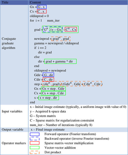
A solution to reducing computation time is to use multiple threads on the GPU to calculate the forward/backward operator for each voxel in parallel because the computations for each voxel are independent. Our CG implementation is composed of several subfunctions, including the forward operator, the backward operator, sparse matrix multiplications, and dot products.
In the implementation of the CG algorithm, the most computationally intensive operations are the matrix-vector multiplications involving
G
and
G
H
. Other than the forward/backward operators, significant computational slowdown occurs if data is transferred between the CPU and the GPU before and after each call to the forward/backward operators. For example, a data transfer time of 157 ms was observed for a dataset with
N
= 64
2
. This is a large amount of time relative to the computation time, which was 0.152 ms for the forward operator with this dataset (on an NVIDIA G80 GPU). This suggests that all CG computations should be ported to the GPU, with data stored in GPU memory. This can tremendously reduce the data transfer between the GPU and CPU during the CG iterations.
Note that a transpose sparse matrix-vector multiplication is not needed because switching rows and columns in the sparse matrix representation reduces the problem to just sparse matrix-vector multiplication. As a result, we conclude that there are five CUDA-based kernels that need to be implemented. They are (1) the forward operator, (2) the backward operator, (3) a sparse matrix-vector multiplication, (4) a vector dot product, and (5) vector-vector addition. For simplicity, we describe only two of the important functions in this chapter, namely, the backward operator (the forward operator implementation is similar), and the regularization term with a sparse representation. Additional implementation details can be found by examining the code distributed with this book
[24]
.
44.3.2. High-Speed Implementations of the Iterative CG Algorithm on GPU
In this section, we describe the important functions for high-speed implementation of the CUDA-based image reconstruction on the GPUs. We mainly focus on the implementation of the two kernels, which are the most representative in terms of GPU technique: the backward operator function and the regularization term (which uses sparse matrix representation). The brute-force approach to the calculation of the modified Fourier forward/backward transform operators is a good match to the low-memory bandwidth and high-computational capacity of GPU-based implementations, and it eliminates the need for any interpolation approaches in order to include the additional physics in the signal model. In addition, we briefly describe a multi-GPU implementation for reconstruction of multiple slices.
Kernel Functions on the GPU
In our MRI application, we applied several well-known CUDA optimization techniques from levels of algorithm implementation to program coding style and performance tuning. Regarding algorithmic level optimization, we first analyzed the overall program execution process on a CPU and located two hot spots, the forward/backward kernels, which take nearly 100% of the whole execution time. However, as mentioned earlier, because we need multiple iterations for each slice (e.g., eight iterations in the example used in this chapter), data are potentially transferred back and forth to the GPU side several times. This justifies our choice to move the data to the GPU memory and perform all calculations on the GPU.
Backward Operator
The simplified code segment of the backward operator function is shown in
Figure 44.3
. The outer loop processes each voxel, and the inner loop performs the calculations for each voxel with time-consuming mathematical operations (e.g., multiplication, division, and sin/cos functions). As mentioned earlier, the computation for each image-space voxel is independent of the computation for the other voxels, and thus, is a good match for parallel programming on the GPU.
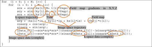 |
| Figure 44.3
Backward operator in conjugate gradient algorithm.
|
To further optimize, the implementation groups together data variables, such as fm, fmgx, fmgy, and fmgz (the magnetic field map and susceptibility gradients the X, Y, Z directions) to benefit from memory coalescing because they are often fetched together. And kx, ky, and kz (k-space sampling trajectories in kx, ky, kz directions) are placed in constant memory to speed up memory access time. An additional consideration for the memory implementation is data tiling. For example, let us assume that the number of image-space voxels is
N
= 64
2
, and the number of k-space samples is
M
= 3770 (for spiral sampling trajectory). For kx, ky, and kz (three vectors with 3770 samples each, and 4 bytes of storage for each sample), storage uses 45,240 bytes (3770 × 3 × 4 bytes), which almost fills up the 64 kB of constant memory available on an NVIDIA G80 GPU. And this case is small compared with typical clinical datasets. Data tiling in constant memory, coincident with coalescing commonly fetched variables, solves this problem. We list some of the main optimizations in the following to improve the GPU performance.
1. Use fast hardware math functions to replace sin and cos. This could cause some accuracy loss, but speeds up the computation significantly. We have previously shown that there is no significant decrease in accuracy from the use of the fast hardware math functions in
[23]
.
2. Take advantage of memory coalescence by storing variables used by the same portion of code in a structure.
3. Replace the division operations with right-shift operations.
4. Group kx, ky, and kz and store them as a structure in constant memory with a data tiling technique if their size exceeds the constant memory capacity.
5. Use registers to hold variables with multiple uses, like kData_r and kData_i (the real and imagi-nary parts of the complex k-space data from the acquisition).
6. Use multiple GPUs for reconstruction of multiple slices to further parallelize the computations (this avoids communication between GPUs, since reconstruction of a given slice is completely independent from reconstruction of the other slices).
Additionally, though not currently implemented, additional optimizations could potentially further increase the performance.
7. Unroll the loop to remove additional branch instructions and use double buffering to get better mixing of computation and memory accesses. However, when using this technique, one must be aware that the number of needed registers will increase and that could lower the number of active blocks on an SM.
8. Dividing the kernel into two parts could lower the computation to memory access ratio (the original ratio is 32/15 if taking
sin/cos
as one operation), but allows for reuse of the constant memory for the second half kernel. For example, we could let the first four statements,
scx
,
scy
,
scz
, and
arg
be the first half kernel and the remaining be the second half kernel. Then, we can reuse constant memory to store
kData_r
and
kData_i
. This method can be applied in conjunction with method 7.
Table 44.2
shows a summary of optimizations used in different versions of our MRI Toolset.
Sparse-Matrix Vector Multiplication (SpMV)
Sparse matrix-vector multiplications are widely used for many scientific computations, such as graph algorithms
[1]
, graphics processing
[2]
and
[3]
, numerical analysis
[10]
and conjugate gradients
[14]
. This problem is essentially a simple multiplication task where the worst case (dense matrix) has a complexity of
O
(N
3
). The key feature of the problem is that the majority of the elements of the matrix are zero and do not require explicit computation. In this section, we will focus on the format-selection according to sparse data format. We surveyed several recent research works on SpMV done on NVIDIA GPU platforms, including
[1]
[2]
[3]
[4]
[5]
and
[8]
. The algorithms for SpMV are greatly affected by the sparse matrix representation so we considered several popular formats, such as the Intel MKL and BSR (block compressed sparse row) sparse matrix storage formats
[10]
, CSR (Compressed Sparse Row)
[8]
and CSC (Compressed Sparse Column) formats, and Matrix Market Coordinate Format (MMCF)
[14]
. We aim at finding a balance between programmability for parallelism and efficiency for speed. The main objective of these representations is to remove the redundant elements (namely, zero values), while keeping the representations readable, easy to manipulate, and compact enough during operations to handle extremely large matrix sizes. Because each format is designed for specific matrix characteristics in order to have the best performance, it is important to choose the right format. For our application, we chose the CSR format and the corresponding GPU CSR vector kernel implementation.
In the CSR vector kernel, the nonzero elements of each row in a matrix are served by one warp (32 threads). Thus, each row is manipulated in the unit of 32 nonzero elements, and 32 multiplication results are added into the final sum of each row. Therefore, if the standard deviation of the numbers of nonzeros in all rows is higher than a warp size, the load imbalance can degrade performance. Each row of the sparse matrix in our regularization term contains roughly a similar number of nonzero elements. This is due to the form of the spatial regularization, which places local constraints on neighboring voxels. Because of this characteristic, the CSR format is very suitable for our case because little load imbalance can happen. Developers should choose a suitable sparse matrix format based on their application.
Multi-GPU Implementation
The multi-GPU-based MRI reconstruction method is implemented on an NVIDIA Tesla S1070 that contains four GT200 GPUs. As mentioned earlier, to reduce the problem of memory bandwidth bottlenecks caused by communications between the GPU and CPU, we reconstruct each slice of the MRI data on one GPU. Therefore, a multithread approach is employed. Each CPU thread is assigned a slice to process, and a GPU that will be used for the kernels. Assignments are designed to preserve a balanced load for all GPUs, as shown in
Figure 44.4
. We are currently working on a dynamic queue to optimize this multi-GPU implementation. This dynamic queue will replace static assignment of slices to GPUs by dynamically dispatching slices to available GPUs
[20]
. Significant improvement is expected to be obtained, especially if the GPUs have different performance levels.
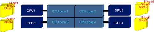 |
| Figure 44.4
Assignment is designed to keep a balanced load among multi-GPUs (e.g., four GPUs connected with a quad-core CPU).
|
44.3.3. MATLAB Toolbox for MRI Reconstruction
In order to allow easy use of our GPU reconstruction program, we have developed a MATLAB (a widely used computational environment
[13]
) toolbox to perform GPU-enabled reconstruction and conveniently visualize the reconstruction results without exporting binary files from the reconstruction program to a separate visualization program. The first part of the toolbox consists of a MATLAB interface to the GPU program (Figure 44.5
). This interface aims to decrease the effort required for new users to start using the reconstruction code, and increase the likelihood of widespread use of our code (in particular) and GPUs in MRI reconstructions (in general). By incorporating the reconstruction code into MATLAB, the iterative reconstruction can be called from MATLAB as part of a complex program (including data pre- or post-processing) with little effort. Additionally, we provide visualization tools (Figure 44.6
) for MATLAB along with export tools to common visualization formats.
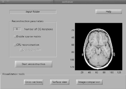 |
| Figure 44.5
MATLAB graphic user interface (GUI) to perform iterative MR image reconstruction from MATLAB.
|
 |
| Figure 44.6
Visualization functions in the advanced MR imaging toolbox.
|
44.4. Final Results and Evaluation
In this section, we present the results obtained with our GPU-based reconstruction method. The CPU and GPU code from our MRI Toolset version 0.1 is available at
[24]
. In this release, we applied the techniques of tiling with constant memory, loop invariant code motion, storing variables in registers, and using single-precision floating-point computations on the GPU kernels. In the CPU kernels, we tried to use OpenMP to parallelize the CPU reconstruction because it accelerates processing time for CPU code. However, the error rate caused by an OpenMP-enabled CPU kernel was not acceptable compared with that of the single-thread version. The normalized root mean squared error measured between CPU and GPU reconstruction was around
10
−3
when using a single-threaded CPU code, and up to around
0.03
when using OpenMP.
For evaluation, a computation time comparison between CPUs and GPUs is shown in
Table 44.3
(for matrix size of 64
2
with 8 iterations). This comparison uses our MRI Toolset v0.2a, running on a dual-core AMD Opteron Processor 2216 (CPU) and an NVIDIA GTX 280 (GPU). As shown in
Table 44.3
, the speedups of our implementation (for the advanced MRI reconstruction) on the GPU reach
398x
compared with a single-thread-enabled CPU, and
105x
compared with a four-thread-enabled CPU.
44.5. Conclusion and Future Directions
Through the use of GPU hardware, we were able to accelerate an advanced image reconstruction algorithm for MRI from around a minute to around a tenth of a second. This reconstruction speed would provide images in the time frames necessary for clinical application. Thus, the use of GPUs will enable improved trade-offs between data acquisition time, signal-to-noise ratio, and the severity of artifacts owing to nonideal physical effects during the MRI imaging experiment.
Follow-up directions include CUDA-based parallel programming on GPUs for an advanced MR imaging reconstruction method combining field inhomogeneity compensation with parallel imaging (e.g., the SENSE algorithm
[17]
). In parallel imaging, information is collected simultaneously from multiple receivers, and this additional information can be used to significantly reduce sampling requirements and greatly accelerate data acquisition.
References
[1]
R.E. Bank, C.C. Douglas,
SMMP: Sparse matrix multiplication package
,
Adv. Comput. Math.
1
(1993
)
127
–
137
.
[2]
N. Bell, M. Garland, Efficient Sparse Matrix-Vector Multiplication on CUDA, NVIDIA Technical Report NVR-2008-004, December 2008.
[3]
J. Bolz, I. Farmer, E. Grinspun, P. Schroder,
Sparse matrix solvers on the GPU: conjugate gradients and multigrid
,
ACM Trans. Graph.
22
(3
) (2003
)
917
–
924
.
[4]
L. Buatois, G. Caumon, B. Lévy,
Concurrent number cruncher — A GPU implementation of a general sparse linear solver
,
Int. J. Parallel, Emergent Distrib. Syst.
24
(3
) (2009
)
205
–
223
.
[5]
M. Christen, O. Schenk, H. Burkhart, General-Purpose Sparse Matrix Building Blocks using the NVIDIA CUDA Technology Platform, Book of Abstracts for First Workshop on General Purpose Processing on Graphics Processing Units, October 4, 2007, Boston.
[6]
J.A. Fessler,
Penalized weighted least-squares image reconstruction for positron emission tomography
,
IEEE Trans. Med. Imaging
13
(2
) (1994
)
290
–
300
.
[7]
J.A. Fessler, S. Lee, V.T. Olafsson, H.R. Shi, D.C. Noll,
Toeplitz-based iterative image reconstruction for MRI with correction for magnetic field inhomogeneity
,
IEEE Trans. Signal Process,
53
(9
) (2005
)
3393
–
3402
.
[8]
M. Garland,
Sparse matrix multiplications on manycore GPU's
,
In:
Proceedings of the 45th Annual Conference on Design Automation, Annual ACM IEEE Design Automation Conference, 8–13 June 2008
Anaheim, ACM, New York
. (2008
), pp.
2
–
6
.
[9]
G.H. Glover,
3D z-shim method for reduction of susceptibility effects in BOLD fMRI
,
Magn. Reson. Med.
42
(2
) (1999
)
290
–
299
.
[10]
Intel Corporation
,
Sparse Matrix Storage Formats
,
http://www.intel.com/software/products/mk1/docs/webhelp/appendices/mk1_appA_SMSF.html
.
[11]
J.I. Jackson, C.H. Meyer, D.G. Nishimura, A. Macovski,
Selection of a convolution function for Fourier inversion using gridding
,
IEEE Trans. Med. Imaging
10
(3
) (1991
)
473
–
478
.
[12]
G. Liu, S. Ogawa,
EPI image reconstruction with correction of distortion and signal losses
,
J. Magn. Reson. Imaging
24
(3
) (2006
)
683
–
689
.
[13]
Matlab,
http://www.mathworks.com/products/matlab
.
[14]
The Matrix Market, Website:
http://math.nist.gov/MatrixMarket/
.
[15]
D.C. Noll, C.H. Meyer, J.M. Pauly, D.G. Nishimura, A. Macovski,
A homogeneity correction method for magnetic resonance imaging with time-varying gradients
,
IEEE Trans. Med. Imaging
10
(4
) (1991
)
629
–
637
.
[16]
D.C. Noll, J.A. Fessler, B.P. Sutton,
Conjugate phase MRI reconstruction with spatially variant sample density correction
,
IEEE Trans. Med. Imaging
24
(3
) (2005
)
325
–
336
.
[17]
K.P. Pruessmann, M. Weiger, M.B. Scheidegger, P. Boesiger,
SENSE: Sensitivity encoding for fast MRI
,
Magn. Reson. Med.
42
(1999
)
952
–
962
.
[18]
K. Sekihara, K. Masao, H. Kohno,
Image restoration from non-uniform magnetic field influence for direct Fourier NMR imaging
,
Phys. Med. Biol.
29
(10
) (1984
)
15
–
24
.
[19]
S.S. Stone, J.P. Haldar, S.C. Tsao, W.W. Hwu, B.P. Sutton, Z.-P. Liang,
Accelerating advanced MRI reconstructions on GPUs
,
J. Parallel Distrib. Comput.
68
(2008
)
1307
–
1318
.
[20]
J. Stone, J. Saam, D.J. Hardy, K.L. Vandivort, W.W. Hwu, K. Schulten,
High performance computation and interactive display of molecular orbitals on GPUs and multi-core CPUs
,
In:
Washington, DC, ACM, New York
.
ACM International Conference Proceeding Series, 8 March 2009
,
vol. 383
(2009
), pp.
9
–
18
.
[21]
B.P. Sutton, D.C. Noll, J.A. Fessler,
Fast, iterative image reconstruction for MRI in the presence of field inhomogeneities
,
IEEE Trans. Med. Imaging
22
(2
) (2003
)
178
–
188
.
[22]
Y. Zhuo, B.P. Sutton,
Effect on BOLD sensitivity due to susceptibility-induced echo time shift in spiral-in based functional MRI
,
In:
Proc of IEEE Engineering in Med and Biol Society 2009, 2–6 September 2009
Minneapolis, IEEE, Piscataway, NJ
. (2009
), pp.
4449
–
4452
.
[23]
Y. Zhuo, X. Wu, J.P. Haldar, W. Hwu, Z. Liang, B.P. Sutton,
Multi-GPU Implementation for Iterative MR Image Reconstruction with Field Correction
,
In:
Proceedings of International Society for Magnetic Resonance in Medicine (ISMRM 2010), 1–7 May 2010
(2010
)
Stockholm
, p.
2942
.
[24]
Y. Zhuo, X. Wu, J.P. Haldar, W. Hwu, Z. Liang, B.P. Sutton, GPU/CPU Code is available for download at the following Web sites:
http://impact.crhc.illinois.edu/mri.php
or
http://mrfil.bioen.illinois.edu/index_files/code.htm
.
..................Content has been hidden....................
You can't read the all page of ebook, please click here login for view all page.