
Chapter 43. Using GPUs to Learn Effective Parameter Settings for GPU-Accelerated Iterative CT Reconstruction Algorithms
Wei Xu and Klaus Mueller
43.1. Introduction, Problem Statement, and Context
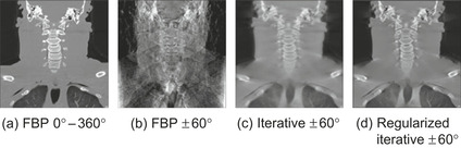
In computed tomography (CT), the filtered backprojection (FBP) algorithm is most widely used for the reconstruction of an object from its X-ray projections. It considers each projection only once and is therefore fast to compute. FBP requires a great number of projection images to be acquired, and within a highly constrained scanning orbit. Recently, more awareness has been placed on reducing the patient X-ray dose. This limits the number of projection images per scan, among other factors. Here, FBP methods are less applicable and iterative reconstruction methods produce significantly better results (Figure 43.1
). However, iterative methods are computationally expensive, but they are now becoming feasible owing to the vast computational performance of GPUs.
 |
| Figure 43.1
Reconstructions of the visible human neck area, coronal cuts. (a) FBP − 360 projections, 0∘ – 360∘, (b) FBP −60 projections, ±60∘, (c) iterative− 60 projections, ±60∘, (d) regularized iterative−60 projections, ±60∘.
|
Iterative methods typically offer a diverse set of parameters that allow control over quality and computation speed, often requiring trade-offs. The interactions among these parameters can be complex, and thus effective combinations can be difficult to identify for a given data scenario. As a result their choice is often left to educated guesses, which in most cases leads to suboptimal speed and quality performance. In addition, we have also found that the specific parallel architecture of GPUs further influences this parameter optimization, modifying some of this conventional wisdom.
Determining the optimal parameter settings, similar to iterative CT reconstruction, is a high-dimensional search problem, and we seek to make this search computationally feasible with GPUs taking part in this process. We further aim to learn these optimal parameter settings in the context of specific imaging tasks and then port these settings to other similar imaging scenarios to achieve equally optimal results.
43.2. Core Method(s)
As an interesting observation in the context of parallel computation, we have found
[11]
that iterative reconstruction methods used in medical imaging, such as EM (expectation maximization) or algebraic methods, such as SIRT (simultaneous iterative reconstruction method), have special properties when it comes to their acceleration on GPUs. This is particularly well expressed when the data is divided in subsets, with each forming an atomic iterative step in a so-called
ordered subsets
algorithm. Although splitting the data used within each iterative update into a larger number of smaller subsets has long been known to offer greater convergence and computation speed on the CPU, it can be vastly slower on the GPU. This is a direct consequence of the thread fill rate in the projection and backprojection phase. Larger subsets spawn a greater number of threads, which keeps the pipelines busier and also reduces the latencies incurred by a greater number of passes and context switches. This is different from the behavior on CPUs where this decomposition is less relevant in terms of computation overhead per iteration. So we seek to optimize the number of subsets for best speed of computation.
On the other hand, from a quality perspective the best subset size is one that most optimally balances the noise compensation offered by larger subsets (many projections in one subset) and the smaller number of iterations required for convergence offered by smaller subsets (many corrective updates within one iteration). Having noticed that on GPUs the speed of convergence is not necessarily related to actual wall clock time, our focus was to provide a mechanism by which one can balance GPU
runtime performance
(which is convergence as measured in wall-clock time) with noise cancelation (for better reconstruction quality).
A second parameter that can be used to mitigate noise effects in the data is to co-optimize the relaxation factor for the iterative updates (see the discussion later in this chapter). It can be used to restore the theoretical convergence advantage of data decompositions into smaller ordered subsets. Finally, using only a small number of projections in the backprojection causes streak artifacts, whereas noisy projections acquired in low-dose acquisition modes lead to a significant amount of noise in the reconstructions. Both can be reduced by ways of regularization between iterative updates. Regularization entails an edge-preserving smoothing operation, which also has parameters that trade quality and speed.
We describe a framework that not only targets GPU-acceleration of iterative reconstruction algorithms but also exploits GPUs to optimize their parameters for a given quality/speed performance objective. In essence we use GPUs to help us reason about GPUs within a machine-learning framework. Our optimization procedure exploits fast GPU-based computation to generate computation products that it then automatically evaluates using a perceptually based fitness function, implementing a simulated human observer, together with the recorded execution time, to steer the optimization.
We offer two different approaches. In the first, we compute a large number of CT reconstructions for all possible parameter combinations and then search this population to recommend parameter settings under two different labeling criteria: (1) “best quality, given a certain time limit” or (2) “best reconstruction speed, given a certain quality threshold.” A weighting scheme is applied to combine the candidate parameters: either a fast-decaying Gaussian function or the max function. In the second approach, we treat the problem as a multi-objective optimization problem, optimizing the settings for desired speed/quality trade-off (or compromise). Genetic algorithms are well suited for this class of problems. Instead of computing all parameter combinations beforehand, we randomly generate a subset as the initial population and then guide the creation of new generations with selection, recombination, and mutation operators on the parameter settings, improving the fitness values until the nondominated optimal solutions set has been determined. With this approach, the suggested parameters are no longer one specific value, but a group of mutually nondominated values comprising objectives. Both approaches require a massive number of reconstructions to be computed, which is only economically feasible with GPU support. Finally, besides the two approaches, an interactive parameter selection interface is introduced to assist evaluation of the behavior of different parameter settings.
43.3. Algorithms, Implementations, and Evaluations
43.3.1. GPU-Accelerated Iterative Ordered-Subset Algorithms
Iterative CT reconstruction methods can broadly be categorized into projection onto convex sets (POCS) algorithms and statistical algorithms. The method we devised, OS-SIRT
[7]
, is a generalization of the simultaneous algebraic reconstruction technique (SART)
[2]
and the simultaneous iterative reconstruction technique (SIRT)
[4]
, two traditional iterative algorithms belonging to the first category. It groups the projections into a number of equal-size subsets and for each subset, iteratively applies the three-phase computation — forward projection, corrective update computation, and backprojection until convergence. We describe this algorithm next.
Most iterative CT techniques use a projection operator to model the underlying image-generation process at a certain viewing configuration (angle) φ. The result of this projection simulation is then compared with the acquired image obtained at the same viewing configuration. If scattering or diffraction effects are ignored, the modeling consists of tracing a straight ray
r
i
from each image element (pixel) and summing the contributions of the (reconstruction) volume elements (voxels)
v
i
. Here, the weight factor
w
ij
determines the contribution of a
v
j
to
r
i
and is given by the interpolation kernel used for sampling the volume. The projection operator is given as
 where
M
and
N
are the number of rays (one per pixel) and voxels, respectively. Because GPUs are heavily optimized for computing and less for memory bandwidth, computing the
w
ij
on the fly, via bilinear interpolation (possibly using the GPU fixed-function pipelines), is by far more efficient than storing the weights in memory. The correction update is computed with the following equation:
where
M
and
N
are the number of rays (one per pixel) and voxels, respectively. Because GPUs are heavily optimized for computing and less for memory bandwidth, computing the
w
ij
on the fly, via bilinear interpolation (possibly using the GPU fixed-function pipelines), is by far more efficient than storing the weights in memory. The correction update is computed with the following equation:

(43.1)
(43.2)
Here, the
p
i
are the pixels in the
M/S
acquired images that form a specific (ordered) subset
OS
s
where 1 ≤
s
≤
S
and
S
is the number of subsets. The factor λ is the relaxation factor that scales the corrective update to each voxel (reducing oscillations). The factor
k
is the iteration count, where
k
is incremented each time all
M
projections have been processed. In essence, all voxels
v
j
on the path of a ray
r
i
are updated (corrected) by the difference of the projection ray
r
i
and the acquired pixel
p
i
, where this correction factor is first normalized by the sum of weights encountered by the (backprojection) ray
r
i
. Because a number of backprojection rays will update a given
v
j
, these corrections need also to be normalized by the sum of (correction) weights. In practice, only the forward projection uses a ray-driven approach, where each ray is a parallel thread and interpolates the voxels on its path. Conversely, the backprojection uses a voxel-driven approach, where each voxel is a parallel thread and interpolates the correction image. Thus, the weights used in the projection and the backprojection are slightly different, but this turns out to be of less importance in practice.
The high performance of GPUs stems from its multicore structure, enabling parallel execution of a sufficiently large number of SIMD (single instruction, multiple data) computing threads. Each such thread must have a target that eventually receives the outcome of the thread's computation. In the forward projection the targets are the pixels on the projection images receiving the outcome of the ray integrations (Eq. 43.1
). The corrective update computation is a simple weighted subtraction operation between computed and scanned projections that has the same targets as forward projections. In the backprojection the targets are the reconstructed volume voxels receiving the corrective updates (Eq. 43.2
). At any phase, the computation of each target (pixel or voxel) is independent of the outcomes of other targets. This feature allows us to manage the three phases as three passes in the GPU and inside each pass the threads with corresponding targets can be executed in parallel. For details, the reader is referred to our papers
[7]
[8]
[9]
[10]
and
[11]
.
43.3.2. GPU-Accelerated Regularization for OS-SIRT
A regularization step is needed when the reconstruction becomes severely ill posed, in cases when the data is sparse or the angular coverage is limited. This is often the case in low-dose CT applications. The regularization operator is added as the fourth phase to “clean up” the intermediate reconstruction between iterations. Here, the targets are the volume voxels and the computation can also be accelerated on the GPU. We have used the bilateral filter (BF) to remove noise and streaking artifacts that emerge in these situations, while at the same time keeping sharp edges as the salient features. The bilateral filter uses a combination of two Gaussians as a weighting function to average the values inside a target voxel neighborhood. One of the Gaussian functions operates as a domain filter to measure the spatial difference, while the other operates as a range filter to measure the pixel value difference. Because the BF-filter is noniterative, it is by nature much faster than the (iterative) TVM algorithm and, as shown earlier in this chapter, offers the same or even better regularization results, except in extremely noisy situations.
43.3.3. Approach 1: Learning Effective Reconstruction Parameters Using Exhaustive Sampling
With the projection data, we compute a representative set of reconstructions, sampling the parameter space in a comprehensive manner. The parameters include number of subsets
S
, the relaxation factor λ, and number of iterations. If the regularization operator is applied, then three more parameters are added: two Gaussian standard deviations and a neighborhood size. We then evaluate these reconstructions with a perceptual quality metric as discussed later in this chapter to obtain a fitness (quality) score for each reconstruction. Adaptive sampling can be used to drive the data collection into more “interesting” parameter regions (those that produce more diverse reconstruction results in terms of the quality metrics). Therefore, each reconstruction has both a quality score and a computation time. Having acquired these observations, we label them according to certain criteria, such as “quality, given a certain wall-clock time limit,” or “reconstruction speed, given a certain quality threshold.” The observations with the higher marks, according to some grouping, subsequently receive higher weights in determining the reconstruction algorithm parameters. Currently, we either use the max function or a fast-decaying Gaussian function to produce this weighting.
43.3.4. Approach 2: Learning Effective Reconstruction Parameters Using Multi-Objective Optimization
For OS-SIRT, the best quality and minimum time are the two objectives that are conflicting in nature with one another. Essentially, there is no single solution to satisfy every objective. Finding the optimal solutions is to make good compromises or trade-offs of the objectives. Therefore, this parameter-learning problem is actually a multi-objective optimization (MOO)
[3]
[4]
and
[5]
. Generally speaking, there are two classes of approaches to this problem: combining objective functions to a single composite function or determining a nondominated optimal solution set (a so-called Pareto optimal set). The kernel of Approach 1 described previously belongs to the former class of multi-objective optimization problems. The two objectives are weighted together to form a single objective function by selecting different labeling criteria. However, when the user does not have a specific quality or time demand, but is curious about the level of potential progress toward each objective when the reconstruction continues, a nondominated Pareto optimal set is more helpful and reasonable.
To solve the MOO problems, genetic algorithms (GA) are well suited. Genetic algorithms inspired by the evolutionary theory about the origin of species have been developed for decades. They mimic the species evolutionary process in nature that strong species have higher opportunity to pass down their genes to the next generations, and at the same time, random changes may occur to bring additional advantages. By natural selection, the weak genes will be eliminated eventually. GA operates in a similar way by evolving from a population with individuals representing initial solutions with operators such as selection, crossover, and mutation to create descending generations. The fitness function is used to evaluate an individual that determines its probability of survival for the next generation. For MOO several fitness functions are used. Numerous GA methods have been described, such as weighted-based genetic algorithm (WBGA), vector evaluated genetic algorithm (VEGA), multi-objective genetic algorithm (MOGA), and nondominated sorting genetic algorithm (NSGA)
[3]
. Approach 1 is a customized application of the combination of fitness functions of WBGA to accommodate our special requirements. VEGA is limited owing to the “middling” problem, whereas MOGA is highly dependent on an appropriate selection of the sharing factor. NSGA progresses more slowly than MOGA and is shown to be computationally inefficient.
In our work, we have selected NSGA-II
[1]
, which is the improved version of NSGA as the method to find the Pareto optimal set. This method uses elitism and a crowded comparison operator to keep both the inheritance from well-performing chromosomes and the diversity of the found optimal solutions, while keeping the computational efficiency. We execute the learning process in this way: after generating the initial population, the reconstruction algorithm OS-SIRT and the parameter searching algorithm NSGA-II are run alternatively until the stopping criterion has been satisfied (for instance, after a sufficient number of generations). This scheme falls into the category of a master-slave model of parallel genetic algorithms
[6]
. Within each generation, OS-SIRT is executed as a parallel fitness values evaluator, while NSGA-II combines these values to find the current solution set with a user-defined set size. Time is recorded as one objective and reconstruction quality is evaluated by a perceptual metric E-CC introduced later in this chapter. To cast the optimization into a minimization problem, we modify the quality metric to its distance to unity. The process stops until the solutions in the current set are nondominated to each other. For the selection, crossover, and mutation operators, we use binary tournament selection, real coded blend crossover, and a nonuniform mutation. Although the parameters we found may not be substantially better for a specific user demand, they provide a pool of candidates that are trade-offs of time and quality. More important, they are obtained considerably faster because fewer reconstructions need to be computed. With Approach 1 we need to perform every combination of the representative parameters, whereas with Approach 2, the computational complexity is the number of generations multiplying twice the size (user defined) of Pareto optimal solutions, which is usually much smaller.
43.3.5. Perceptual Metric as Automated Reconstruction Quality Evaluator
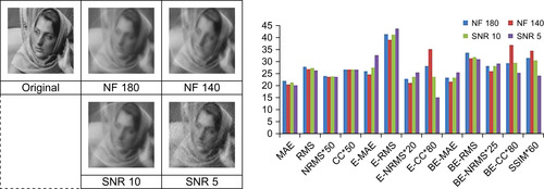
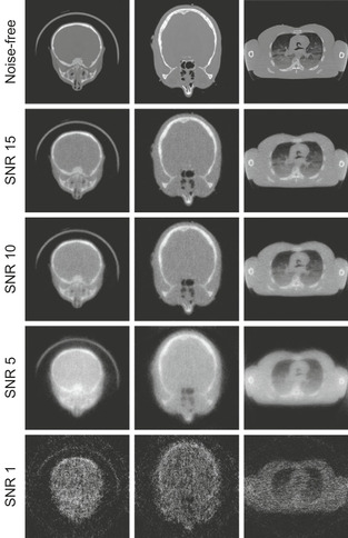
As mentioned before, a reliable quality metric is needed to evaluate the reconstruction results. Most popular for the assessment of image quality in CT have been statistical metrics such as mean absolute error (MAE), root mean square (RMS), normalized RMS (NRMS), cross-correlation coefficient (CC), and R-factor. However, these metrics do not consider the fact that human vision is highly sensitive to structural information. These properties are well captured in the gradient domain, by ways of an edge-filtered image calculated via a Sobel Filter operator. We have labeled this group of metrics by prefix E-. Further, shifting effects caused by the CT reconstruction backprojection step can be alleviated by Gaussian-blurring the reconstruction image before edge filtering. We have labeled this group of metrics with prefix “BE-.” Another method to gauge structural information is structural similarity (SSIM), which combines luminance, contrast, and structure
[8]
.
We tested the evaluation of these methods with four images whose rankings are determined by a human observer (in the order NF 140, NF 180, SNR 10, SNR 5, with NF 140 being the best) shown in
Figure 43.2
. Only the edge-based metrics (E-MAE, E-NRMS, and E-CC), as well as SSIM, can reproduce this ranking. In this chapter, the E-CC metric standing for the CC of two edge images is used as the perceptual quality metric as automated human observer owing to its efficiency in computation.
 |
| Figure 43.2
A metrics comparison.
|
43.3.6. An Interactive Parameter Selection Interface
Users often like to see what will happen when some parameters are slightly changed to express their personal trade-offs better. We devised an effective parameter space navigation interface
[10]
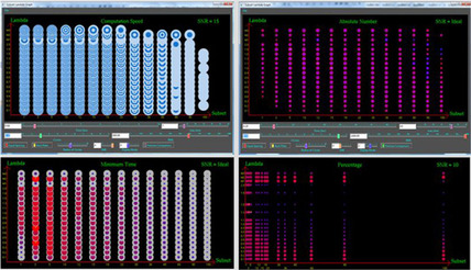
allowing users to interactively assist parameter selection for iterative CT reconstruction algorithms (here for OS-SIRT). It is based on a 2-D scatter plot with six display modes to show different features of the reconstruction results based on user preferences. It also enables a dynamic visualization by gradual parameter alteration for illustrating the rate of impact of a given parameter constellation.
For OS-SIRT, there are seven parameters to represent one reconstruction: SNR-level, relaxation factor λ, number of subsets S, number of iterations, time, CC, and RMS. With the given projections, we selected a representative set of integer subsets, λ(plus three simulated relaxation factor functions) and SNR-levels, respectively. For each combination of “<
S
, λ, SNR-level > ” (called grid points), <time, CC, RMS> (called tuples) were recorded every five iterations. With this pool of tuples, we use our parameter space visualizer to visualize the parameters with user control.
The interface of the parameter space visualizer is composed of a main window and a control panel (see the first row of
Figure 43.3
). The main window is a 2-D scatter plot of number of subsets (x coordinate) and relaxation factor (y coordinate) with different sizes and colors of circles to show the features of tuples. The size and color of the circle represent the number of tuples satisfying current parameter settings controlled by users in the control panel. In the control panel, users could change the values of the time, CC, and RMS bars to set boundary values to sift tuples and switch visualizations among different SNR-levels. There are six modes showing various features of the tuples: computation speed mode, percentage mode, absolute number mode, minimum time mode, maximum CC mode, and starting CC mode. The interface assists users to quickly find the preferred parameter settings and provide a dynamic view of parameter changes by moving the control bars.
 |
| Figure 43.3
Parameter space navigator.
|
43.4. Final Evaluation and Validation of Results, Total Benefits, and Limitations
In this section, we tested the performance for every algorithm mentioned previously: the OS-SIRT reconstruction with regularization and the two parameter learning approaches. All computations used an NVIDIA GTX 280 GPU/Intel 2 Quad CPU 2.66 GHz. Cg/GLSL with OpenGL API is used for the coding of GPU acceleration parts.
43.4.1. Performance Gains of Our Iterative CT Reconstruction Algorithms
An application where very large volumes are frequently reconstructed from projections is electron microscopy. Here, the maximal dose (and therefore number of projection images) is limited by the amount of energy that the biological specimen can tolerate before decomposition. This application forms an excellent test bed for our high-performance iterative reconstruction framework.
We find that our GPU-accelerated iterative ordered-subset (OS) algorithm is able to decrease the running time from hours to minutes for the reconstruction large 3-D volumes.
Tables 43.1
and
43.2
demonstrate the speedup for both 2-D (Table 43.1
comparing ours with timing reported by others) and 3-D (Table 43.2
)
[11]
. The reconstruction results for SART (N subsets of size 1 projection), SIRT (1 subset with size N projections), and our ordered subsets SIRT (OS-SIRT) with the optimal number of subsets, 5 (OS-SIRT 5), as determined by our optimization procedure, are shown in
Figure 43.4
.
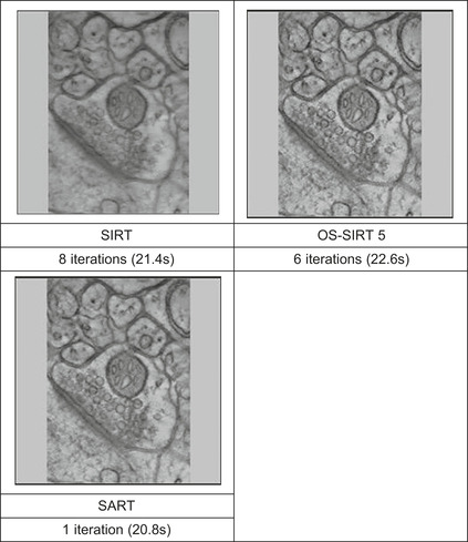 |
| Figure 43.4
Comparing electron microscopy reconstructions (HPFcere2 dataset) obtained at similar wall-clock times, but different qualities (OS-SIRT 5 is best).
|
Figure 43.5
compares the three different algorithms (SIRT, OS-SIRT 5, and SART) quantitatively using the R-factor (the R-factor compares the absolute error of the actual projections with the simulated projections). Although the R-factor still improves beyond the images we have shown here, we found that these improvements are not well perceived visually, and so, we have not shown these images here. To visualize the aspect of computational performance in the context of a quantitative reconstruction quality measure (here, the R-factor), we have inserted into
Figure 43.5
a metric that we call the “computation time iso-contour.” Here, we used 22s for this contour — the approximate time required for 1 SART, 6 OS-SIRT, and 8 SIRT iterations (see
Figure 43.4
), which yielded reconstructions of good quality for OS-SIRT 5. We observe that OS-SIRT 5 offers a better time-quality performance than SART, and this is also true for other such time iso-contours (although not shown here) because the time per iteration for OS-SIRT is roughly 1/6 of that for SART. SIRT, on the other hand, converges at a much higher R-factor.
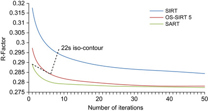 |
| Figure 43.5
Comparing different subsets algorithms in terms of speed and quality. The 22s iso-contour shows that OS-SIRT achieves the best quality (R-factor).
|
43.4.2. Performance Gains of Our Regularization Scheme
As mentioned, for few-view, limited-angle, and noisy projection scenarios, the application of regularization operators between reconstruction iterations seeks to tune the final or intermediate results to some a priori model. Total variation minimization (TVM) is a commonly used method for medical imaging regularization. It has the effect of flattening the density profile in local neighborhoods and thus is well suited for noise and streak artifact reduction. However, in the context of high-performance computing, owing to its iterative procedure, TVM is quite time-consuming, even when accelerated on GPUs. To speed up the computation we aim to devise a method that is not iterative, but has the same goals as TVM, that is, the reduction of local variations (noise, streaks) while preserving coherent local features. We found that a bilateral filtering (BF) scheme can behave just as good or better than TVM, but without the need for iterative application. In our scheme each kernel performs a convolution operation inside a neighborhood with two textures used as lookup tables of weights to combine the nearby and similar pixels. The performances of CPU and GPU are compared in
Table 43.3
. We observe that GPU acceleration leads to speedups of two orders of magnitude, reducing it to only 10% of an iterative update, making regularization a computationally affordable operation. The effects of filtering for both BF and TVM are shown in
Figure 43.6
[9]
.
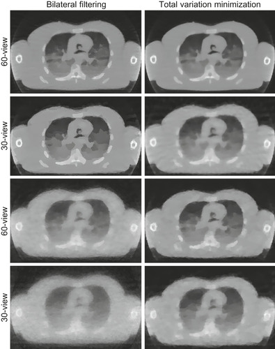 |
| Figure 43.6
A slice of a CT few-view reconstructed torso with lung: (top two rows) noise free; (bottom two rows) SNR 10.
|
43.4.3. Performance of Approach 1
To test the effectiveness of the learned parameters using Approach 1, we first simulated, from the test image (here is baby head CT scan), 180 projections at uniform angular spacing of [−90∘, +90∘] in a parallel projection viewing geometry. We then added different levels of Gaussian noise to the projection data to obtain SNRs (signal-noise ratio) of 15, 10, 5, and 1. The first column of
Figure 43.7
presents the best reconstruction results (using the E-CC between the original and the reconstructed image) for each SNR in terms of the “reconstruction speed, given a certain quality threshold” criterion. In other words, the images shown are the reconstructions that could be obtained at the shortest wall-clock time given a certain minimal E-CC constraint. This constraint varies for each projection dataset (low SNR cannot reach high E-CC levels), and this is also part of the process model.
Figure 43.8
summarizes the various parameters obtained for the various aforementioned data scenarios. The “Best Subset” and “Best λ” values denote the parameter settings that promise to give the best results, in terms of the given quality metric and label criterion. The “Lowest λ” and “Turning Point” values describe the shape of the λ-curve as a function of the number of subsets. The λ-factor is always close to 1 for small subsets and then linearly (as an approximation) falls off at the “Turning Point” to value “Lowest λ” when each subset only consists of one projection.
 |
| Figure 43.7
Applying learned parameter settings for different imaging scenarios.
|
 |
| Figure 43.8
Optimal learned parameter settings for different SNR.
|
We then explored if the knowledge we learned translates to other similar data and reconstruction scenarios. Columns 2 and 3 of
Figure 43.7
show the results obtained when applying the optimal settings learned from the baby head to reconstructions of the visible human head (size 265
2
) and visible human lung (512
2
), from similar projection data. We observe that the results are quite consistent with those obtained with the baby head, and this is promising. As future work, we plan to compare the settings with those learned directly from these two candidate datasets.
43.4.4. Performance of Approach 2
To test the performance of the second approach, the visible human head (size 256
2
) with different noise levels (ideal, SNR 10, and SNR 5) is used. We set the size of any Pareto optimal set to 20 and obtained the corresponding sets for parameters (number of iterations, number of subsets, and relaxation factor λ) after adequate generations (here until any solution is nondominated by others in the same set). The results for different noise levels are shown in
Figure 43.9
. For each noise level, the gradual evolutions of the fitness values after a selected number of generations are plotted. We observed that when the generation develops, the fitness values are closer to the axes that means closer to its optimal value. The solutions pool is listed in
Table 43.4
. It demonstrates that when the noise level increases the reconstruction is more difficult, while at the same time, the needed numbers of iterations and subsets are getting smaller. This is confirmed by Approach 1 as well
[8]
.
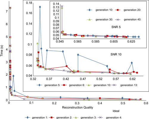 |
| Figure 43.9
Fitness values of solutions set evolutions for different SNR.
|
43.5. Future Directions
In this chapter, we introduced a framework based on a GPU-accelerated iterative reconstruction platform with regularization to search the optimal parameter settings for the reconstruction process itself satisfying multiple performance objectives. In essence, we use GPUs to help us reason about GPUs within a machine-learning framework. As future work, the machine-learning procedure could further be accelerated in GPUs, and the regularization parameters could also be studied in the same way. We believe that our parameter-learning approach has many more general applications than shown here. Parameters are commonplace in many applications, and finding optimal settings for these can be a laborious task. By using GPUs to test all possible parameter settings in parallel, optimal settings can be found fast and accurately. Because the result we optimize is ultimately meant for human consumption, an important component we have devised and integrated into our optimization framework is the simulated human observer. At the same time, we also use the interactive performance of GPUs to allow users to formulate and test trade-offs on the fly, by way of the parameter visualization framework that we also presented here.
References
[1]
K. Deb, S. Agrawal, A. Pratap, T. Meyarivan,
A fast elitist non-dominated sorting genetic algorithm for multi-objective optimization: NSGA-II
,
In:
Proceedings of the Sixth International Conference on Parallel Problem Solving from Nature (PPSN VI), 18–20 September 2000
(2000
)
Springer
,
Paris, France
, pp.
849
–
858
.
[2]
A.H. Andersen, A.C. Tarjan,
Simultaneous algebraic reconstruction technique (SART): a superior implementation of the ART algorithm
,
Ultrason. Imaging
6
(1984
)
81
–
94
.
[3]
C.A. Coello,
A short tutorial on evolutionary multiobjective optimization
,
In:
Proceedings of the 1st International Conference Evolutionary Multi-Criterion Optimization (EMO'01), 7–9 March 2001
(2001
)
Springer-Verlag
,
Zurich, Switzerland
, pp.
21
–
40
.
[4]
P. Tarjan,
Iterative methods for the 3D reconstruction of an object from projections
,
J. Theor. Biol.
36
(1
) (1972
)
105
–
117
.
[5]
A. Konak, D.W. Coit, A.E. Smith,
Multi-objective optimization using genetic algorithms: a tutorial
,
Reliab. Eng. Syst. Saf. (Special Issue – Genetic Algorithms and Reliability)
91
(9
) (2006
)
992
–
1007
.
[6]
E. Cantu-Paz, A Survey of Parallel Genetic Algorithms, Technical Report 97003, Illinois Genetic Algorithms Laboratory, Department of General Engineering, University of Illinois, Urbana, Illinois, 1997.
[7]
F. Xu, W. Xu, M. Jones, B. Keszthelyi, J. Sedat, D. Agard, K. Mueller,
On the efficiency of iterative ordered subset reconstruction algorithms for acceleration on GPUs
,
Comput. Methods Programs Biomed.
98
(3
) (2010
)
261
–
270
.
[8]
W. Xu, K. Mueller,
Learning effective parameter settings for iterative CT reconstruction algorithms
,
In:
10th International Meeting on Fully Three-Dimensional Image Reconstruction in Radiology and Nuclear Medicine (Fully3D'09) 5–10 September 2009
Beijing China
. (2009
), pp.
251
–
254
.
[9]
W. Xu, K. Mueller,
A performance-driven study of regularization methods for PU-accelerated iterative CT
,
In:
10th International Meeting on Fully Three-Dimensional Image Reconstruction in Radiology and Nuclear Medicine, 2nd High Performance Image reconstruction Workshop (HPIR'09)
Beijing China
. (6 September 2009
), pp.
20
–
23
.
[10]
W. Xu, K. Mueller,
Parameter space visualizer: an interactive parameter selection interface for iterative CT reconstruction algorithms
,
In:
San Diego, CA, SPIE, Bellingham, WA
.
SPIE on Medical Imaging, 13–18 February 2010
,
vol. 7625
(2010
), p.
76251Q
.
[11]
W. Xu, F. Xu, M. Jones, B. Keszthelyi, J. Sedat, D. Agard,
et al.
,
High-performance iterative electron tomography reconstruction with long-object compensation using Graphics Processing Units (GPUs)
,
J. Struct. Biol.
171
(2
) (2010
)
142
–
153
.
..................Content has been hidden....................
You can't read the all page of ebook, please click here login for view all page.