
Chapter 1. GPU-Accelerated Computation and Interactive Display of Molecular Orbitals
John E. Stone, David J. Hardy, Jan Saam, Kirby L. Vandivort and Klaus Schulten
In this chapter, we present several graphics processing unit (GPU) algorithms for evaluating molecular orbitals on three-dimensional lattices, as is commonly used for molecular visualization. For each kernel, we describe necessary design trade-offs, applicability to various problem sizes, and performance on different generations of GPU hardware. We then demonstrate the appropriate and effective use of fast on-chip GPU memory subsystems for access to key data structures, show several GPU kernel optimization principles, and explore the application of advanced techniques such as dynamic kernel generation and just-in-time (JIT) kernel compilation techniques.
1
1
This work was supported by the National Institutes of Health, under grant
P41-RR05969
. Portions of this chapter © 2009 Association for Computing Machinery, Inc. Reprinted by permission
[1]
.
1.1. Introduction, Problem Statement, and Context
The GPU kernels described here form the basis for the high-performance molecular orbital display algorithms in VMD
[2]
, a popular molecular visualization and analysis tool. VMD (Visual Molecular Dynamics) is a software system designed for displaying, animating, and analyzing large biomolecular systems. More than 33,000 users have registered and downloaded the most recent VMD software, version 1.8.7. Due to its versatility and user-extensibility, VMD is also capable of displaying other large datasets, such as sequence data, results of quantum chemistry calculations, and volumetric data. While VMD is designed to run on a diverse range of hardware — laptops, desktops, clusters, and supercomputers — it is primarily used as a scientific workstation application for interactive 3-D visualization and analysis. For computations that run too long for interactive use, VMD can also be used in a batch mode to render movies for later use. A motivation for using GPU acceleration in VMD is to make slow batch-mode jobs fast enough for interactive use, thereby drastically improving the productivity of scientific investigations. With CUDA-enabled GPUs widely available in desktop PCs, such acceleration can have a broad impact on the VMD user community. To date, multiple aspects of VMD have been accelerated with the NVIDIA Compute Unified Device Architecture (CUDA), including electrostatic potential calculation, ion placement, molecular orbital calculation and display, and imaging of gas migration pathways in proteins.
Visualization of molecular orbitals (MOs) is a helpful step in analyzing the results of quantum chemistry calculations. The key challenge involved in the display of molecular orbitals is the rapid evaluation of these functions on a three-dimensional lattice; the resulting data can then be used for plotting isocontours or isosurfaces for visualization as shown in
Fig. 1.1
and for other types of analyses. Most existing software packages that render MOs perform calculations on the CPU and have not been heavily optimized. Thus, they require runtimes of tens to hundreds of seconds depending on the complexity of the molecular system and spatial resolution of the MO discretization and subsequent surface plots.
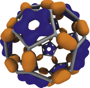 |
| Figure 1.1
An example of MO isovalue surfaces resulting from the lattice of wavefunction amplitudes computed for a Carbon-60 molecule. Positive valued isosurfaces are shown in dark grey, and negative valued isosurfaces are shown in light grey.
|
With sufficient performance (two orders of magnitude faster than traditional CPU algorithms), a fast real-space lattice computation enables interactive display of even very large electronic structures and makes it possible to smoothly animate trajectories of orbital dynamics. Prior to the use of the GPU, this could be accomplished only through extensive batch-mode precalculation and preloading of time-varying lattice data into memory, making it impractical for everyday interactive visualization tasks. Efficient single-GPU algorithms are capable of evaluating molecular orbital lattices up to 186 times faster than a single CPU core (see
Table 1.1
), enabling MOs to be rapidly computed and animated on the fly for the first time. A multi-GPU version of our algorithm has been benchmarked at up to 419 times the performance of a single CPU core (see
Table 1.2
).
| Device | CPU Workers | Runtime (sec) | Speedup vs. Q6600 | Speedup vs. X5550 | Multi-GPU Efficiency depth5pt |
|---|---|---|---|---|---|
| Quadro 5800 | 1 | 0.381 | 122 | 80 | 100.0% |
| Tesla C1060 | 2 | 0.199 | 234 | 154 | 95.5% |
| Tesla C1060 | 3 | 0.143 | 325 | 214 | 88.6% |
| Tesla C1060 | 4 | 0.111 | 419 | 276 | 85.7% |
1.2. Core Method
Since our target application is visualization focused, we are concerned with achieving interactive rendering performance while maintaining sufficient accuracy. The CUDA programming language enables GPU hardware features — inaccessible in existing programmable shading languages — to be exploited for higher performance, and it enables the use of multiple GPUs to accelerate computation further. Another advantage of using CUDA is that the results can be used for nonvisualization purposes.
Our approach combines several performance enhancement strategies. First, we use the host CPU to carefully organize input data and coefficients, eliminating redundancies and enforcing a sorted ordering that benefits subsequent GPU memory traversal patterns. The evaluation of molecular orbitals on a 3-D lattice is performed on one or more GPUs; the 3-D lattice is decomposed into 2-D planar slices, each of which is assigned to a GPU and computed. The workload is dynamically scheduled across the pool of GPUs to balance load on GPUs of varying capability. Depending on the specific attributes of the problem, one of three hand-coded GPU kernels is algorithmically selected to optimize performance. The three kernels are designed to use different combinations of GPU memory systems to yield peak memory bandwidth and arithmetic throughput depending on whether the input data can fit into constant memory, shared memory, or L1/L2 cache (in the case of recently released NVIDIA “Fermi” GPUs). One useful optimization involves the use of zero-copy memory access techniques based on the CUDA mapped host memory feature to eliminate latency associated with calls to
cudaMemcpy()
. Another optimization involves dynamically generating a problem-specific GPU kernel “on the fly” using just-in-time (JIT) compilation techniques, thereby eliminating various sources of overhead that exist in the three general precoded kernels.
A molecular orbital (MO) represents a statistical state in which an electron can be found in a molecule, where the MO's spatial distribution is correlated with the associated electron's probability density. Visualization of MOs is an important task for understanding the chemistry of molecular systems. MOs appeal to the chemist's intuition, and inspection of the MOs aids in explaining chemical reactivities. Some popular software tools with these capabilities include MacMolPlt
[3]
, Molden
[4]
, Molekel
[5]
and VMD
[2]
.
The calculations required for visualizing MOs are computationally demanding, and existing quantum chemistry visualization programs are only fast enough to interactively compute MOs for only small molecules on a relatively coarse lattice. At the time of this writing, only VMD and MacMolPlt support multicore CPUs, and only VMD uses GPUs to accelerate MO computations. A great opportunity exists to improve upon the capabilities of existing tools in terms of interactivity, visual display quality, and scalability to larger and more complex molecular systems.
1.3.1. Mathematical Background
In this section we provide a short introduction to MOs, basis sets, and their underlying equations. Interested readers are directed to seek further details from computational chemistry texts and review articles
[6]
and
[7]
. Quantum chemistry packages solve the electronic Schrödinger equation
H
Ψ =
E
Ψ for a given system. Molecular orbitals are the solutions produced by these packages. MOs are the eigenfunctions Ψ
ν
for expression of the molecular wavefunction Ψ, with
H
the Hamiltonian operator and
E
the system energy. The wavefunction determines molecular properties, for instance, the one-electron density is
ρ
(r
) = |Ψ(r
)|
2
. The visualization of the molecular orbitals resulting from quantum chemistry calculations requires evaluating the wavefunction on a 3-D lattice so that isovalue surfaces can be computed and displayed. With minor modifications, the algorithms and approaches we present for evaluating the wavefunction can be adapted to compute other molecular properties such as charge density, the molecular electrostatic potential, or multipole moments.
Each MO Ψ
ν
can be expressed as a linear combination over a set of
K
basis functions Φ
κ
,
 where
c
νκ
are coefficients contained in the quantum chemistry calculation output files, and used as input for our algorithms. The basis functions used by the vast majority of quantum chemical calculations are atom-centered functions that approximate the solution of the Schrödinger equation for a single hydrogen atom with one electron, so-called atomic orbitals. For increased computational efficiency, Gaussian type orbitals (GTOs) are used to model the basis functions, rather than the exact solutions for the hydrogen atom:
where
c
νκ
are coefficients contained in the quantum chemistry calculation output files, and used as input for our algorithms. The basis functions used by the vast majority of quantum chemical calculations are atom-centered functions that approximate the solution of the Schrödinger equation for a single hydrogen atom with one electron, so-called atomic orbitals. For increased computational efficiency, Gaussian type orbitals (GTOs) are used to model the basis functions, rather than the exact solutions for the hydrogen atom:
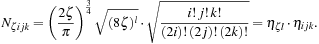
 The exponential factor
ζ
is defined by the basis set;
i
,
j
, and
k
are used to modulate the functional shape; and
N
ζijk
is a normalization factor that follows from the basis set definition. The distance from a basis function's center (nucleus) to a point in space is represented by the vector
R
= {
x
,
y
,
z
} of length
R
= |
R
|.
The exponential factor
ζ
is defined by the basis set;
i
,
j
, and
k
are used to modulate the functional shape; and
N
ζijk
is a normalization factor that follows from the basis set definition. The distance from a basis function's center (nucleus) to a point in space is represented by the vector
R
= {
x
,
y
,
z
} of length
R
= |
R
|.
(1.1)
(1.2)
The exponential term in
Eq. 1.2
determines the radial decay of the function. Composite basis functions known as contracted GTOs (CGTOs) are composed of a linear combination of
P
individual GTO
primitives
in order to accurately describe the radial behavior of atomic orbitals.
(1.3)
CGTOs are classified into different
shells
based on the sum
l
=
i
+
j
+
k
of the exponents of the
x
,
y
, and
z
factors. The shells are designated by letters s, p, d, f, and g for
l
= 0, 1, 2, 3, 4, respectively, where we explicitly list here the most common shell types but note that higher-numbered shells are occasionally used. The set of indices for a shell is also referred to as the
angular momenta
of that shell. We establish an alternative indexing of the angular momenta based on the shell number
l
and a systematic indexing
m
over the possible number of sums
l
=
i
+
j
+
k
, where
 counts the number of combinations and
m
= 0, …,
M
l
− 1 references the set
counts the number of combinations and
m
= 0, …,
M
l
− 1 references the set
 .
.
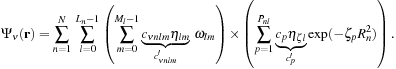
The linear combination defining the MO Ψ
ν
must also sum contributions from each of the
N
atoms of the molecule and the
L
n
shells of each atom
n
. The entire expression, now described in terms of the
data output from a QM package, for an MO wavefunction evaluated at a point
r
in space then becomes
 where we have replaced
c
νκ
by
c
νnlm
, with the vectors
R
n
=
r
−
r
n
connecting the position
r
n
of the nucleus of atom
n
to the desired spatial coordinate
r
. We have dropped the subscript
p
from the set of contraction coefficients {
c
} and exponents {
ζ
} with the understanding that each CGTO requires an additional summation over the primitives, as expressed in
Eq. 1.3
.
where we have replaced
c
νκ
by
c
νnlm
, with the vectors
R
n
=
r
−
r
n
connecting the position
r
n
of the nucleus of atom
n
to the desired spatial coordinate
r
. We have dropped the subscript
p
from the set of contraction coefficients {
c
} and exponents {
ζ
} with the understanding that each CGTO requires an additional summation over the primitives, as expressed in
Eq. 1.3
.
(1.4)
The normalization factor
N
ζijk
in
Eq. 1.2
can be factored into a first part
η
ζl
that depends on both the exponent
ζ
and shell type
l
=
i
+
j
+
k
and a second part
η
ijk
(=
η
lm
in terms of our alternative indexing) that depends only on the angular momentum,
 The separation of the normalization factor in
Eq. 1.5
allows us to factor the summation over the primitives from the summation over the array of wavefunction coefficients. Combining
(1.2)
(1.3)
and
(1.4)
and rearranging terms gives
The separation of the normalization factor in
Eq. 1.5
allows us to factor the summation over the primitives from the summation over the array of wavefunction coefficients. Combining
(1.2)
(1.3)
and
(1.4)
and rearranging terms gives
 We define
 using our alternative indexing over
l
and
m
explained in the previous section. Both data storage and operation count can be reduced by defining
using our alternative indexing over
l
and
m
explained in the previous section. Both data storage and operation count can be reduced by defining
 and
and
 . The number of primitives
P
nl
depends on both the atom
n
and the shell number
l
.
Figure 1.2
shows the organization of the basis set and wavefunction coefficient arrays listed for a small example molecule.
. The number of primitives
P
nl
depends on both the atom
n
and the shell number
l
.
Figure 1.2
shows the organization of the basis set and wavefunction coefficient arrays listed for a small example molecule.
(1.5)
(1.6)
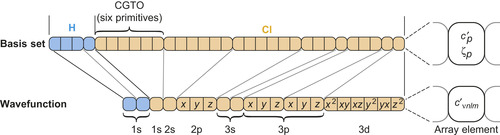 |
| Figure 1.2
Structure of the basis set and the wavefunction coefficient arrays for HCl using the 6-31G* basis
[8]
. Each rounded box contains the data for a single shell. Each square box in the basis set array represents a CGTO primitive composed of a contraction coefficient
c
′
p
and exponent
ζ
p
. In the wavefunction array the elements signify linear combination coefficients
c
′
νnlm
for the basis functions. Despite the differing angular momenta, all basis functions of a shell (marked by
x
,
y
, and
z
) use the same linear combination of primitives (see lines relating the two arrays). For example, the 2p shell in Cl is associated with three angular momenta that all share the exponents and contraction coefficients of the same six primitives. There can be more than one basis function for a given shell type (brackets below array). © 2009 Association for Computing Machinery, Inc. Reprinted by permission
[1]
.
|
1.3.2. GPU Molecular Orbital Algorithms
Visualization of MOs requires the evaluation of the wavefunction on a 3-D lattice, which can be used to create 3-D isovalue surface renderings, 3-D height field plots, or 2-D contour line plots within a plane. Since wavefunction amplitudes diminish to zero beyond a few Angstroms (due to the radial decay of exponential basis functions), the boundaries of the 3-D lattice have only a small margin beyond the bounding box containing the molecule of interest.
The MO lattice computation is heavily data dependent, consisting of a series of nested loops that evaluate the primitives composing CGTOs and the angular momenta for each shell, with an outer loop over atoms. Since the number of shells can vary by atom and the number of primitives and angular momenta can be different for each shell, the innermost loops traverse variable-length coefficient arrays
containing CGTO contraction coefficients and exponents, and the wavefunction coefficients. Quantum chemistry packages often produce output files containing redundant basis set definitions for atoms of the same species; such redundancies are eliminated during preprocessing, resulting in more compact data and thus enabling more effective use of fast, but limited-capacity on-chip GPU memory systems for fast access to key coefficient arrays. The memory access patterns that occur within the inner loops of the GPU algorithms can be optimized to achieve peak performance by carefully sorting and packing coefficient arrays as a preprocessing step. Each of the coefficient arrays is sorted on the CPU so that array elements are accessed in a strictly consecutive pattern. The pseudo-code listing in
Algorithm 1
summarizes the performance-critical portion of the MO computation described by
Eq. 1.6
.
The GPU MO algorithm decomposes the 3-D lattice into a set of 2-D planar slices, which are computed independently of each other. In the case of a single-GPU calculation, a simple
for
loop processes the slices one at a time until they are all completed. For a multi-GPU calculation, the set of slices is dynamically distributed among the pool of available GPUs. Each of the GPUs requests a slice index to compute, computes the assigned slice, and stores the result at the appropriate location in host memory.
Each planar slice computed on a GPU is decomposed into a 2-D CUDA grid consisting of fixed-size 8 × 8 thread blocks. As the size of the 3-D lattice increases, the number of planar slices increases, and the number of thread blocks in each CUDA grid increases accordingly. Each thread is responsible for computing the MO at a single lattice point. For lattice dimensions that cannot be evenly divided by the thread block dimensions or the memory coalescing size, padding elements are added (to avoid unnecessary branching or warp divergence). The padding elements are computed just as the interior lattice points are, but the results are discarded at the end of the computation.
Figure 1.3
illustrates the multilevel parallel decomposition strategy and required padding elements.
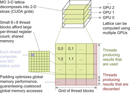 |
| Figure 1.3
Molecular orbital multilevel parallel decomposition. The 3-D MO lattice is decomposed into 2-D planar slices that are computed by the pool of available GPUs. Each GPU computes a single slice, decomposing the slice into a grid of 8 × 8 thread blocks, with each thread computing one MO lattice point. Padding elements are added to guarantee coalesced global memory accesses for lattice data.
|
1: Ψ
ν
⇐ 0.0
2:
ifunc
⇐ 0 {index the array of wavefunction coefficients)
3:
ishell
⇐ 0 {index the array of shell numbers}
4:
for
n
= 1 to
N
do
{loop over atoms}
5:
(x
,
y
,
z
) ⇐
r
−
r
n
(r
n
is position of atom
n
}
6:
R
2
⇐
x
2
+
y
2
+
z
2
7:
iprim
⇐
atom_basis
[
n
] {index the arrays of basis set data}
8:
for
l
= 0
to num_shells_per_atom
[
n
] − 1} {loop over shells}
9:
Φ
CGTO
⇐ 0.0
10:
for
p
= 0 to
num_prim_per_shell
[
ishell
] − 1
do
{loop over primitives}
11:
c
′
p
⇐
basis_c
[
iprim
]
12:
ζ
p
⇐
basis_zeta
[
iprim
]
13:
Φ
CGTO
⇐ Φ
CGTO
+
c
′
p
e
−
ζpR
2
14:
iprim
⇐
iprim
+ 1
15:
end for
16:
for all
0 ≤
i
≤
shell_type
[
ishell
]
do
{loop over angular momenta}
17:
jmax
⇐
shell_type
[
ishell
] −
i
18:
for all
0 ≤
j
≤
jmax
do
19:
k
⇐
jmax
−
j
20:
c
′ ⇐
wavefunction
[
ifunc
]
21:
Ψ
ν
⇐ Ψ
ν
+
c
′ Φ
CGTO
x
i
y
j
z
k
22:
ifunc
⇐
ifunc
+ 1
23:
end for
24:
end for
25:
ishell
⇐
ishell
+ 1
26:
end for
26:
end for
27:
return
Ψ
ν
In designing an implementation of the MO algorithm for the GPU, one must take note of a few key attributes of the algorithm. Unlike simpler forms of spatially evaluated functions that arise in molecular modeling such as Coulombic potential kernels, the MO algorithm involves a comparatively large number of floating-point operations per lattice point, and it also involves reading operands from several different arrays. Since the MO coefficients that must be fetched depend on the atom type, basis set, and other factors that vary due to the data-dependent nature of the algorithm, the control flow complexity is also quite a bit higher than for many other algorithms. For example, the bounds on the loops on lines 10 and 16 of
Algorithm 1
are both dependent on the shell being evaluated. The MO algorithm makes heavy use of exponentials that are mapped to the dedicated exponential arithmetic instructions provided by most GPUs. The cost of evaluating
e
x
by calling the CUDA routines
expf()
or
__expf()
, or evaluating 2
x
via
exp2f()
, is much lower than on the CPU, yielding a performance benefit well beyond what would be expected purely as a result of effectively using the massively parallel GPU hardware.
Given the high performance of the various exponential routines on the GPU, the foremost consideration for achieving peak performance is attaining sufficient operand bandwidth to keep the GPU
arithmetic units fully occupied. The algorithms we describe achieve this through careful use of the GPU's fast on-chip caches and shared memory. The MO algorithm's inner loops read varying numbers of coefficients from several different arrays. The overall size of each of the coefficient arrays depends primarily on the size of the molecule and the basis set used. The host application code dispatches the MO computation using one of several GPU kernels depending on the size of the MO coefficient arrays and the capabilities of the attached GPU devices. Optimizations that were applied to all of the kernel variants include precomputation of common factors and specialization and unrolling of the angular momenta loops (lines 16 to 24 of
Algorithm 1
). Rather than processing the angular momenta with loops, a
switch
statement is used that can process all of the supported shell types with completely unrolled loop iterations, as exemplified in the abbreviated source code shown in
Figure 1.4
.
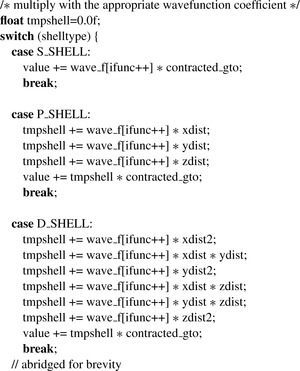 |
| Figure 1.4
Example of completely unrolled shell-type-specific angular momenta code.
|
Constant Cache
When all of the MO coefficient arrays (primitives, wavefunctions, etc.) will fit within 64kB, they can be stored in the fast GPU constant memory. GPU constant memory is cached and provides near-register-speed access when all threads in a warp access the same element at the same time. Since all of the threads in a thread block must process the same basis set coefficients and CGTO primitives, the constant cache kernel source code closely follows the pseudo-code listing in
Algorithm 1
.
Tiled-Shared Memory
If the MO coefficient arrays exceed 64kB in aggregate size, the host application code dispatches a GPU kernel that dynamically loads coefficients from global memory into shared memory as needed, acting
as a form of software-managed cache for arbitrarily complex problems. By carefully sizing shared memory storage areas (tiles) for each of the coefficient arrays, one can place the code for loading new coefficients outside of performance-critical loops, which greatly reduces overhead. Within the innermost loops, the coefficients in a shared memory tile are read by all threads in the same thread block, reducing global memory accesses by a factor of 64 (for 8 × 8 thread blocks). For the outer loops (over atoms, basis set indices, the number of shells per atom, and the primitive count and shell type data in the loop over shells) several coefficients are packed together with appropriate padding into 64-byte memory blocks, guaranteeing coalesced global memory access and minimizing the overall number of global memory reads. For the innermost loops, global memory reads are minimized by loading large tiles immediately prior to the loop over basis set primitives and the loop over angular momenta, respectively. Tiles must be sized to a multiple of the 64-byte memory coalescing size for best memory performance, and power-of-two tile sizes greatly simplify shared memory addressing arithmetic. Tiles must also be sized large enough to provide all of the operands consumed by the loops that follow the tile-loading logic.
Figure 1.5
illustrates the relationship between coalesced memory block sizes, the portion of a loaded array that will be referenced during subsequent innermost loops, and global memory padding and unreferenced data that exist to simplify shared memory addressing arithmetic and to guarantee coalesced global memory accesses.
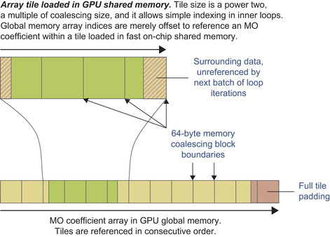 |
| Figure 1.5
Schematic representation of the tiling strategy used to load subsets of large arrays from GPU global memory, into small regions of the high-performance on-chip shared memory. © 2009 Association for Computing Machinery, Inc. Reprinted by permission
[1]
.
|
NVIDIA recently released a new generation of GPUs based on the “Fermi” architecture that incorporate both L1 and L2 caches for global memory. The global memory cache in Fermi-based GPUs enables a comparatively simple kernel that uses only global memory references to run at nearly the speed of the highly tuned constant cache kernel; it outperforms the tiled-shared memory kernel due to the reduction in arithmetic operations encountered within the inner two loop levels of the kernel. The hardware cache kernel can operate on any problem size, with an expected graceful degradation in performance up until the point where the problem size exceeds the cache capacity, at which point it may begin to perform slower than uncached global memory accesses if cache thrashing starts to occur. Even in the situation where the problem size exceeds cache capacity, the strictly consecutive memory access patterns employed by the kernel enable efficient broadcasting of coefficients to all of the threads in the thread block.
Zero-Copy Host-Device I/O
One performance optimization that can be paired with all of the other algorithms is the use of CUDA “host-mapped memory.” Host-mapped memory allocations are areas of host memory that are made directly accessible to the GPU through on-demand transparent initiation of PCI-express transfers between the host and GPU. Since the PCI-e transfers incur significant latency and the PCI-e bus can provide only a fraction of the peak bandwidth of the on-board GPU global memory, this technique is a net win only when the host side buffers are read from or written to only once during kernel execution. In this way, GPU kernels can directly access host memory buffers, eliminating the need for explicit host-GPU memory transfer operations and intermediate copy operations. In the case of the MO kernels, the output lattice resulting from the kernel computation can be directly written to the host output buffer, enabling output memory writes to be fully overlapped with kernel execution.
Since
Algorithm 1
is very data dependent, we observe that most instructions for loop control and conditional execution could be eliminated for a given molecule by generating a molecule-specific kernel at runtime. A significant optimization opportunity exists based on dynamical generation of a molecule-specific GPU kernel. The kernel is generated when a molecule is initially loaded, and may then be reused. The generation and just-in-time (JIT) compilation of kernels at runtime has associated overhead that must be considered when determining how much code to convert from data-dependent form into a fixed sequence of operations. The GPU MO kernel is dynamically generated by emitting the complete arithmetic sequence normally performed by looping over shells, primitives, and angular momenta for each atom type. This on-demand kernel generation scheme eliminates the overhead associated with loop control instructions (greatly increasing the arithmetic density of the resulting kernel) and allows the GPU to perform much closer to its peak floating-point arithmetic rate. At present, CUDA lacks a mechanism for runtime compilation of C-language source code, but provides a mechanism for runtime compilation of the PTX intermediate pseudo-assembly language through a driver-level interface. OpenCL explicitly allows dynamic kernel compilation from C-language source.
To evaluate the dynamic kernel generation technique with CUDA, we implemented a code generator within VMD and then saved the dynamically generated kernel source code to a file. The standard batch-mode CUDA compilers were then used to recompile VMD incorporating the generated CUDA kernel. We have also implemented an OpenCL code generator that operates in much the same way, but the kernel can be compiled entirely at runtime so long as the OpenCL driver supports online compilation. One significant complication with implementing dynamic kernel generation for OpenCL is the need to handle a diversity of target devices that often have varying preferences for the width of vector types, work-group sizes, and other parameters that can impact the structure of the kernel. For simplicity of the present discussion, we present the results for the dynamically generated CUDA kernel only.
1.4. Final Evaluation
The performance of each of the MO algorithms was evaluated on several hardware platforms. The test datasets were selected to be representative of the range of quantum chemistry simulation data that researchers often work with, and to exercise the limits of our algorithms, particularly in the case of the GPU. The benchmarks were run on a Sun Ultra 24 workstation containing a 2.4GHz Intel Core 2 Q6600 quad core CPU running 64-bit Red Hat Enterprise Linux version 4 update 6. The CPU code was compiled using the GNU C compiler (gcc) version 3.4.6 or Intel C/C++ Compiler (icc) version 9.0. GPU benchmarks were performed using the NVIDIA CUDA programming toolkit version 3.0 running on several generations of NVIDIA GPUs.
All of the MO kernels presented have been implemented in either production or experimental versions of the molecular visualization program VMD
[2]
. For comparison of the CPU and GPU implementations, a computationally demanding carbon-60 test case was selected. The
C
60
system was simulated with GAMESS, resulting in an output file (containing all of the wavefunction coefficients, basis set, and atomic element data) that was then loaded into VMD. The MO was computed on a lattice with a 0.075Å spacing, with lattice sample dimensions of 172 × 173 × 169. The
C
60
test system contained 60 atoms, 900 wavefunction coefficients, 15 unique basis set primitives, and 360 elements in the per-shell primitive count and shell type arrays. The performance results listed in
Table 1.1
compare the runtime for computing the MO lattice on one or more CPU cores, and on several generations of GPUs using a variety of kernels.
The CPU “icc-libc” result presented in the table refers to a kernel that makes straightforward use of the
expf()
routine from the standard C library. As is seen in the table, this results in relatively low performance even when using multiple cores, so we implemented our own
expf()
routine. The single-core and multicore CPU results labeled “icc-sse-cephes” were based on a handwritten SIMD-vectorized SSE adaptation of the scalar
expf()
routine from the Cephes
[9]
mathematical library. The SSE
expf()
routine was hand-coded using intrinsics that are compiled directly into x86 SSE machine instructions. The resulting “icc-sse-cephes” kernel has previously been shown to outperform the CPU algorithms implemented in the popular MacMolPlt and Molekel visualization tools, and it can be taken to be a representative peak-performance CPU reference
[1]
.
The single-core CPU result for the “icc-sse-cephes” kernel was selected as the basis for normalizing performance results because it represents the best-case single-core CPU performance. Benchmarking on a single core results in no contention for limited CPU cache or main memory bandwidth, and performance can be extrapolated for an arbitrary number of cores. Most workstations used for scientific visualization and analysis tasks now contain four or eight CPU cores, so we consider the four-core CPU results to be representative of a typical CPU use-case today.
The CUDA “const-cache” kernel stores all MO coefficients within the 64kB GPU constant memory. The “const-cache” kernel can be used only for datasets that fit within fixed-size coefficient arrays within GPU constant memory, as defined at compile time. The “const-cache” results represent the best-case performance scenario for the GPU. The CUDA “tiled-shared” kernel loads blocks of the MO coefficient arrays from global memory using fully coalesced reads, storing them in high-speed on-chip shared memory where they are accessed by all threads in each thread block. The “tiled-shared” kernel supports problems of arbitrary size. The CUDA Fermi “L1-cache (16kB)” kernel uses global memory reads for all MO coefficient data and takes advantage of the Fermi-specific L1/L2 cache hardware to achieve performance exceeding the software-managed caching approach implemented by the “tiled-shared” kernel. The CUDA results for “zero-copy” kernels demonstrate the performance advantage gained by having the GPU directly write orbital lattice results back to host memory rather than requiring the CPU to execute
cudaMemcpy()
operations subsequent to each kernel completion. The CUDA results for the JIT kernel generation approach show that the GPU runs a runtime-generated basis-set-specific kernel up to 1.85 times faster than the fully general loop-based kernels.
All of the benchmark test cases were small enough to reside within the GPU constant memory after preprocessing removed duplicate basis sets, so the “tiled-shared” and “L1-cache (16kB)” test cases were conducted by overriding the runtime dispatch heuristic, forcing execution using the desired CUDA kernel irrespective of problem size.
We ran multi-GPU performance tests on an eight-core system based on 2.6GHz Intel Xeon X5550 CPUs, containing an NVIDIA Quadro 5800 GPU, and three NVIDIA Tesla C1060 GPUs (both GPU types provide identical CUDA performance, but the Tesla C1060 has no video output hardware).
Table 1.2
lists results for a representative high-resolution molecular orbital lattice intended to show scaling performance for a very computationally demanding test case. The four-GPU host benchmarked in
Table 1.2
outperforms the single-core SSE results presented in
Table 1.1
by up to factors of 419 (vs. Q6600 CPU) and 276 (vs. X5550 CPU). The four-GPU host outperforms the eight-core SSE X5550 CPU result by a factor of 37, enabling interactive molecular visualizations that were previously impossible to be achieved with a single machine.
1.5. Future Directions
The development of a range-limited version of the molecular orbital algorithm that uses a distance cutoff to truncate the contributions of atoms that are either far away or that have very rapidly decaying exponential terms can change the molecular orbital computation from a quadratic time complexity algorithm into one with linear time complexity, enabling it to perform significantly faster for display of very large quantum chemistry simulations. Additionally, just-in-time dynamic kernel generation techniques can be applied to other data-dependent algorithms like the molecular orbital algorithm presented here.
References
[1]
J.E. Stone, J. Saam, D.J. Hardy, K.L. Vandivort, W.W. Hwu, K. Schulten,
High performance computation and interactive display of molecular orbitals on GPUs and multi-core CPUs
,
In:
Proceedings for the 2nd Workshop on General-Purpose Processing on Graphics Processing Units
(2009
)
ACM
,
New York
, pp.
9
–
18
;
http://doi.acm.org/10.1145/1513895.1513897
.
[2]
W. Humphrey, A. Dalke, K. Schulten,
VMD – visual molecular dynamics
,
J. Mol. Graph
14
(1996
)
33
–
38
.
[3]
B.M. Bode, M.S. Gordon,
MacMolPlt: a graphical user interface for GAMESS
,
J. Mol. Graph. Model.
16
(3
) (1998
)
133
–
138
.
[4]
G. Schaftenaar, J.H. Nooordik,
Molden: a pre- and post-processing program for molecular and electronic structures
,
J. Comput. Aided Mol. Des.
14
(2
) (2000
)
123
–
134
.
[5]
S. Portmann, H.P. Lüthi,
Molekel: an interactive molecular graphics tool
,
Chimia
54
(2000
)
766
–
770
.
[6]
C.J. Cramer,
Essentials of Computational Chemistry
. (2004
)
John Wiley & Sons, Ltd.
,
Chichester, England
.
[7]
E.R. Davidson, D. Feller,
Basis set selection for molecular calculations
,
Chem. Rev.
86
(1986
)
681
–
696
.
[8]
M.M. Francl, W.J. Pietro, W.J. Hehre, J.S. Binkley, M.S. Gordon, D.J. DeFrees,
et al.
,
Self-consistent molecular orbital methods. XXIII. A polarization-type basis set for second-row elements
,
J. Chem. Phys.
77
(1982
)
3654
–
3665
.
[9]
S.L. Moshier, Cephes Mathematical Library Version 2.8.
http://www.moshier.net/#Cephes
, 2000.
..................Content has been hidden....................
You can't read the all page of ebook, please click here login for view all page.