
Discrete Lifetime Models
Abstract
This chapter is concerned with the current and prospective tools that enable the representation of lifetime data through some model. A major component of such a formulation is to identify the probability distribution of the underlying lifetime. We discuss some possible lifetime distributions and their properties in this chapter. Often, a family of distributions is initially chosen and then a member that adequately describes the features of the data is assumed to be the model. We begin with the Ord family comprising of the binomial, Poisson, negative binomial, hypergeometric, negative hypergeometric and beta-Pascal distributions. The power series family and its subfamily, the Lerch distributions, are considered next. Among the distributions discussed in this class are the Hurwitz zeta, Zipf, Zipf-Manelbrot, Good, geometric, uniform, discrete Pareto, Estoup, Lotka, logarithmic and the zeta models. This is followed by considering the Abel series family consisting of generalized Poisson, quasi-binomial I, quasi-negative binomial, quasi-binomial II, and quasi-logarithmic series distributions. Further, the Lagrangian family, with special reference to the Geeta and generalized geometric models, are also discussed. The reliability characteristics of each of the above families such as hazard rate, mean residual life, characterizations based on relationships between reliability functions, recurrence relations, etc. are discussed. Of special interest in reliability modelling in discrete time is the development of discretized versions of acclaimed continuous life distributions. In this category, we review the works on discrete Weibull I, half-logistic, geometric, inverse-Weibull, generalized exponential, gamma and Lindley models and their reliability aspects. We conclude the discussions by presenting other models that do not belong to the above classifications like the discrete Weibull II and III and the S-distributions.
Keywords
Ord family; Power series distributions; Abel series; Discrete versions of continuous models; Discrete Weibull reliability properties
3.1 Introduction
The main emphasis of this chapter is to present a discussion of the current and prospective tools that enable the representation of lifetime data through some model. A major component in such a formulation is the distribution of the underlying lifetime. Probability distributions facilitate characterization of the uncertainty prevailing in the data set by identification of the patterns of variation. By summarizing the observations into a mathematical form that contains a few unknown parameters, distributions provide a means to the best possible understanding to the basic data generating mechanism. Lifetime distributions, being a probabilistic description of the behaviour of the length of life, is to a marked extent depends on the mode of failure of the device under study. Choice of an appropriate distribution for the data set depends largely on our knowledge about the physical characteristics of the process that give rise to the observations. In some cases, the relationship between the failure mechanism and various concepts encountered in Chapter 2 can be forged. However, many situations, unlike the case of the normal distribution where the central limit theorem affords a bridge between theory and practice, the discrete distributions we confront with are difficult to justify on practical grounds. The real position is that within the range of observations we have in hand, more than one distribution may pass well established goodness-of-fit tests in many cases. Characterization properties, being unique to a specified distribution, are the only exact tools that can identify the correct model. When the sample observations provide evidence of characteristic properties exhibited by reliability functions such as hazard rate, mean residual life, etc., pertaining to a particular model with high accuracy, there is reasonable justification to choose that model. If such a model passes the goodness-of-fit test also, then we have a match between observations and the chosen distribution both in terms of comparable physical properties and statistical validity. In Chapter 2, several examples of this nature were illustrated for modelling real data with some specified distributions. The subsequent sections of this chapter will to present various discrete distributions along with their properties that can be used for modelling and analysis of lifetime data. For a detailed discussion of various aspects of reliability modelling, we refer to Blischke and Murthy (2000).
3.2 Families of Distributions
In the presence of lack of understanding of the data generating mechanism due to insufficient details about the physical characteristics, the investigator has to be content with finding the best approximating distribution from a collection of candidate models. Based on a preliminary assessment of the features of the observations at disposal, mathematical formulation of a suitable model is initially made. A family of distributions that contains enough members with different shapes and varying characteristics can be useful aids in the process of empirical modelling described above.
3.2.1 Ord Family
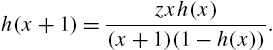
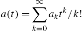
The family of distributions has its origin in 1895 when Pearson introduced a system bearing his name in the continuous case. A discrete version of the Pearson system, defined by the difference equation
was studied by Ord (1967a, 1967b), which is referred to as the Ord family in the sequel, where x takes values in a subset T of integers.
The members of the system with non-negative integers as the values of X are:
- (i) binomial

- (ii) negative binomial

- (iii) Poisson
- (iv) hypergeometric

- (v) negative hypergeometric (beta-binomial)

- (vi) beta-Pascal

-
 ;
;  ;
;  .
.
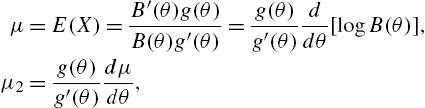
The first four moments of the family are given by
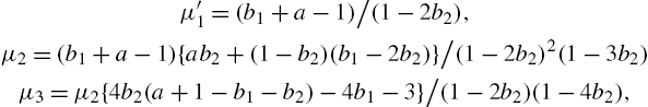
and
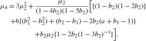
These will be required for analysing the descriptive characteristics of the distribution, estimating parameters by the method of moments, and in computing standard errors of statistics. All distributions of the system are either J shaped or unimodal. A crucial issue of interest when families are considered for model selection, is the criteria to distinguish its members. Ord (1972) considered the quantities ![]() , which is the variance mean ratio called index of dispersion, and
, which is the variance mean ratio called index of dispersion, and ![]() , and proposed a diagram of
, and proposed a diagram of ![]() . In this diagram, the line
. In this diagram, the line ![]() defines the binomial or Poisson or negative binomial distributions as
defines the binomial or Poisson or negative binomial distributions as ![]() . The other distributions are obtained by analyzing
. The other distributions are obtained by analyzing ![]() . The region
. The region ![]() gives the beta-binomial,
gives the beta-binomial, ![]() corresponds to the hypergeometric or beta-Pascal according to whether
corresponds to the hypergeometric or beta-Pascal according to whether ![]() or >1 in addition. Since the parameters of the family are completely determined by the first three moments, the
or >1 in addition. Since the parameters of the family are completely determined by the first three moments, the ![]() diagram can be used to locate a suitable distribution for a given data, by replacing the population moments with the corresponding sample moments. Ord (1972) also proposed the plot of
diagram can be used to locate a suitable distribution for a given data, by replacing the population moments with the corresponding sample moments. Ord (1972) also proposed the plot of ![]() against x, where
against x, where ![]() is the sample frequency. Since successive
is the sample frequency. Since successive ![]() values are dependent, a smoothing
values are dependent, a smoothing ![]() is has also been suggested. For example, the binomial distribution satisfies
is has also been suggested. For example, the binomial distribution satisfies
in the population, so that the plot of ![]() must show an approximate line. An interesting property of the Ord family is that the truncated version of X at either end also belongs to this family.
must show an approximate line. An interesting property of the Ord family is that the truncated version of X at either end also belongs to this family.
Various reliability functions, like the hazard rate, for the Ord family can not be expressed in simple forms. However, the members of the family admit a simple relationship between the hazard rate and the mean residual life. Ahmed (1991) has shown that X has binomial distribution in (3.2) if and only if
Since the mean residual life ![]() , the relationship between
, the relationship between ![]() and
and ![]() characterizing the binomial distribution is obvious. On similar lines, Osaki and Li (1988) have shown that X follows negative binomial distribution
characterizing the binomial distribution is obvious. On similar lines, Osaki and Li (1988) have shown that X follows negative binomial distribution

if and only if
for all integers ![]() . They have also shown that X has Poisson distribution in (3.4) if and only if
. They have also shown that X has Poisson distribution in (3.4) if and only if
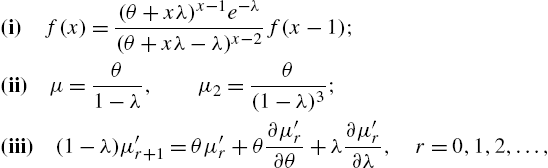
A more general result for the Ord family in (3.1) rewritten as

was characterized by Nair and Sankaran (1991) through the identity
where
The values of ![]() and
and ![]() for the distributions in (3.2)–(3.7) are listed in Table 3.1.
for the distributions in (3.2)–(3.7) are listed in Table 3.1.
Table 3.1
Values of a0,a1 and a2 in (3.9) for the Ord family
| Distribution |
|
|
|
|---|---|---|---|
| binomial | q | q | 0 |
| Poisson | 1 | 1 | 0 |
| negative binomial |
|
|
0 |
| hypergeometric |
|
|
|
| negative hypergeometric |
|
|
|
| beta-Pascal |
|
|
|

Figs 3.1A, 3.1B and 3.1C show the hazard rates of negative binomial, hypergeometric and negative hypergeometric distributions for various values of the parameters.

Various distributional properties of the individual models along with results on inference and applications have been discussed in Johnson et al. (1992). Further, characterization problems of the family in terms of truncated moments have been addressed by Glanzel et al. (1984) and Glanzel (1987, 1991). Of particular interest is the result
in Glanzel (1991), where ![]() and
and ![]() are polynomials of degree at most one, with real coefficients. Obviously, (3.10) leads to a property of the variance residual life in relation to the mean residual life.
are polynomials of degree at most one, with real coefficients. Obviously, (3.10) leads to a property of the variance residual life in relation to the mean residual life.
There are two related families in connection with (3.1) that deserves special mention. One is the Katz (1965) system defined by
It is easy to see that (3.11) is a special case of (3.1) when ![]() ,
, ![]() . This restricted model contains the binomial (
. This restricted model contains the binomial (![]() ), Poisson (
), Poisson (![]() ) and negative binomial (
) and negative binomial (![]() ) distribution as particular members. These members can be discriminated by performing a test of hypothesis
) distribution as particular members. These members can be discriminated by performing a test of hypothesis ![]() against
against ![]() (
(![]() ), with
), with ![]() if accepted gives Poisson, otherwise
if accepted gives Poisson, otherwise ![]() (
(![]() ) gives negative binomial (binomial). The test is based on the statistic
) gives negative binomial (binomial). The test is based on the statistic
which is closely approximated by a normal distribution ![]() , where n is the sample size, and
, where n is the sample size, and ![]() and
and ![]() are the variance and mean of the sample. Following (3.9), for the Katz family, we see that
are the variance and mean of the sample. Following (3.9), for the Katz family, we see that
is satisfied for all x, and conversely. Sudheesh and Nair (2010) established the following characteristic properties for the Ord and Katz families, respectively:
where

and
For example, in the Poisson case, we have
or alternatively in terms of the variance and the hazard rate as
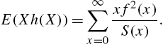
Let τ be the class of real-valued functions ![]() of X. Then, for the Ord family, we have
of X. Then, for the Ord family, we have
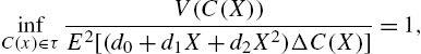
where ![]() and Δ is the forward difference operator,
and Δ is the forward difference operator, ![]() . In particular, for the Katz family, we have
. In particular, for the Katz family, we have

provides the lower bound to the variance of a random function ![]() . Under some regularity conditions, Nair and Sudheesh (2008) showed that these bounds reduce to the Cramer-Rao and Chapman-Robbins inequalities. The moments of the Katz family are
. Under some regularity conditions, Nair and Sudheesh (2008) showed that these bounds reduce to the Cramer-Rao and Chapman-Robbins inequalities. The moments of the Katz family are
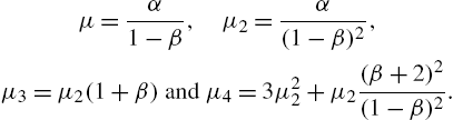
It has a probability generating function
An extension of the Ord family has been provided by Sindhu (2002) wherein the difference equation in (3.1) has the modified form
with ![]() and
and ![]() as real constants. Besides containing all members of the Ord family, the system in (3.14) contains several other distributions such as the confluent hypergeometric distribution of Bhattacharya (1966), Borel-Tanner model (Tanner, 1953), and the Haight distribution (Haight, 1961).
as real constants. Besides containing all members of the Ord family, the system in (3.14) contains several other distributions such as the confluent hypergeometric distribution of Bhattacharya (1966), Borel-Tanner model (Tanner, 1953), and the Haight distribution (Haight, 1961).
Theorem 3.1
A necessary and sufficient condition for the distribution of X to belong to the family in (3.14) is that

Remark 3.1
The approach for relationships between reliability functions in reversed time is the same and very similar results emerge. Corresponding to (3.9), the identity between ![]() and
and ![]() for the Ord family is
for the Ord family is
with ![]() ,
, ![]() and
and ![]() .
.
Gupta et al. (1997) have given a formula for computing the hazard rate as

when the ratio of two successive probabilities are known. By utilizing of this, for the Katz family, we have

where ![]() . An alternative expression is
. An alternative expression is

where ![]() is the hypergeometric function defined as
is the hypergeometric function defined as
with ![]() .
.
For an elaborate study on the orthogonal polynomials in the cumulative Ord family and their application to variance bounds, one may refer to the recent work of Afendras et al. (2017).
3.2.2 Power Series Family
The power series family of distributions were initially studied by Kosambi (1949) and Noack (1950). Any distribution that can be represented as
where ![]() and
and ![]() , is said to be of power series form. In (3.18),
, is said to be of power series form. In (3.18), ![]() is called the series function. Sometimes, (3.18) is also referred to as the discrete linear exponential family in view of the specification of (3.18) as
is called the series function. Sometimes, (3.18) is also referred to as the discrete linear exponential family in view of the specification of (3.18) as
Initially, Noack (1950) considered ![]() with support as the whole set of non-negative integers. Patil (1962) extended the support to any arbitrary non-empty subset T of non-negative integers such that
with support as the whole set of non-negative integers. Patil (1962) extended the support to any arbitrary non-empty subset T of non-negative integers such that
with ![]() ,
, ![]() , so that
, so that ![]() is positive, finite and differentiable. Then, (3.18) for
is positive, finite and differentiable. Then, (3.18) for ![]() is called a generalized power series distribution (GPSD). The system in (3.19) includes the binomial, negative binomial, Poisson and logarithmic series distributions. A truncated GPSD is also a GPSD.
is called a generalized power series distribution (GPSD). The system in (3.19) includes the binomial, negative binomial, Poisson and logarithmic series distributions. A truncated GPSD is also a GPSD.
A further extension of the GPSD has been introduced by Gupta (1974) who defined the modified power series distributions (MPSD), specified by the probability mass function of the form
where ![]() , and
, and ![]() and
and ![]() are positive finite and differentiable. When
are positive finite and differentiable. When ![]() is invertible, MPSD reduces to the GPSD. Apart from all distributions belonging to the GPSD family, the modified version contains more distributions, such as the generalized binomial distribution of Jain and Consul (1971). Being the more general form, the properties of (3.20) will be mentioned so that the results for GPSD can be deduced from them. The moments of (3.20) are
is invertible, MPSD reduces to the GPSD. Apart from all distributions belonging to the GPSD family, the modified version contains more distributions, such as the generalized binomial distribution of Jain and Consul (1971). Being the more general form, the properties of (3.20) will be mentioned so that the results for GPSD can be deduced from them. The moments of (3.20) are
and

The factorial moments can be calculated from the recurrence relation
Consul (1995) has developed characterizations of the exponential family of distributions
which contains numerous discrete probability mass functions and probability density functions of continuous random variables for various choices of ![]() ,
, ![]() and
and ![]() . In the discrete case, the translations
. In the discrete case, the translations ![]() ,
, ![]() and
and ![]() reduce (3.21) to the form (3.20). His main result can be stated in our notation as
reduce (3.21) to the form (3.20). His main result can be stated in our notation as
As examples, the Lagrangian Poisson distribution

satisfies the property

the Lagrangian negative binomial with probability function
is characterized by
Notice that (3.24) contains, as special cases, the binomial distribution (![]() ), negative binomial (
), negative binomial (![]() ), the Geeta distribution
), the Geeta distribution

when ![]() and x is replaced by
and x is replaced by ![]() so that the identity in (3.25) is true for
so that the identity in (3.25) is true for ![]() (binomial), for all x (negative binomial), and
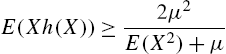
(binomial), for all x (negative binomial), and ![]() (Geeta). The identity in (3.22) can be used to obtain the lower bound for the variance as
(Geeta). The identity in (3.22) can be used to obtain the lower bound for the variance as
when ![]() is any real-valued function of x (Nair and Sudheesh, 2008) and
is any real-valued function of x (Nair and Sudheesh, 2008) and
3.2.3 Lerch Family
An important sub-family of the MPSD is the Hurwitz-Lerch zeta distributions (HLZD). Various properties of this class, along with their applications to reliability, have been studied by Gupta et al. (2008). The HLZD arises from the general Hurwitz-Lerch zeta function defined by

and ![]() when
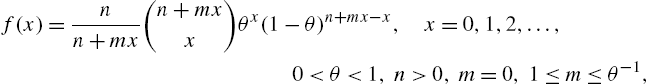
when ![]() and C is the set of complex numbers. Some known special cases of the function (3.26) are the Riemann zeta function
and C is the set of complex numbers. Some known special cases of the function (3.26) are the Riemann zeta function
Hurwitz zeta function
and the polylogarithmic function

For detailed properties of these functions, we refer to Erdelyi et al. (1953). Zornig and Altmann (1995) introduced the three parameter HLZD as a generalization of the Zipf, Zipf-Mandelbrot and Good distributions mentioned below. Subsequently, the family has found some applications as a model in ecology, linguistics, information sciences, statistical physics and survival analysis.
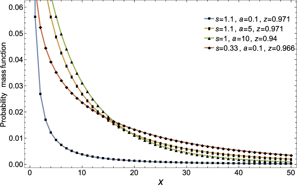
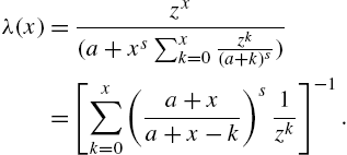
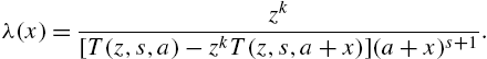
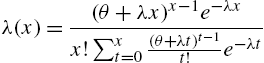
Aksenov and Savageau (2005) defined the Lerch family of distributions through the probability mass function
where ![]() , the Lerch transcendent (Lerch, 1887), also called the Hurwitz-Lerch zeta function defined in (3.26) for
, the Lerch transcendent (Lerch, 1887), also called the Hurwitz-Lerch zeta function defined in (3.26) for ![]() ,
, ![]() . By virtue of the relationship
. By virtue of the relationship

we can arrive at the distribution function
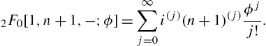
The probability generating function and the moment generating function are, respectively,
and
There is unimodality for the family if ![]() and
and ![]() with mode at
with mode at
where ![]() is the integer part of W. Furthermore,
is the integer part of W. Furthermore,
and
Regarding the reliability functions, we obtain directly from the definitions that

and

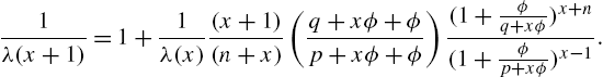
We observe that the expressions in (3.32) leads to some new interesting recurrence relationships and formulae. Since
and
from (3.31), we have on eliminating ϕ between the last two equations,
a recurrence relation for evaluating ![]() . One may use the initial value
. One may use the initial value ![]() in (3.34) to initiate the recurrence.
in (3.34) to initiate the recurrence.
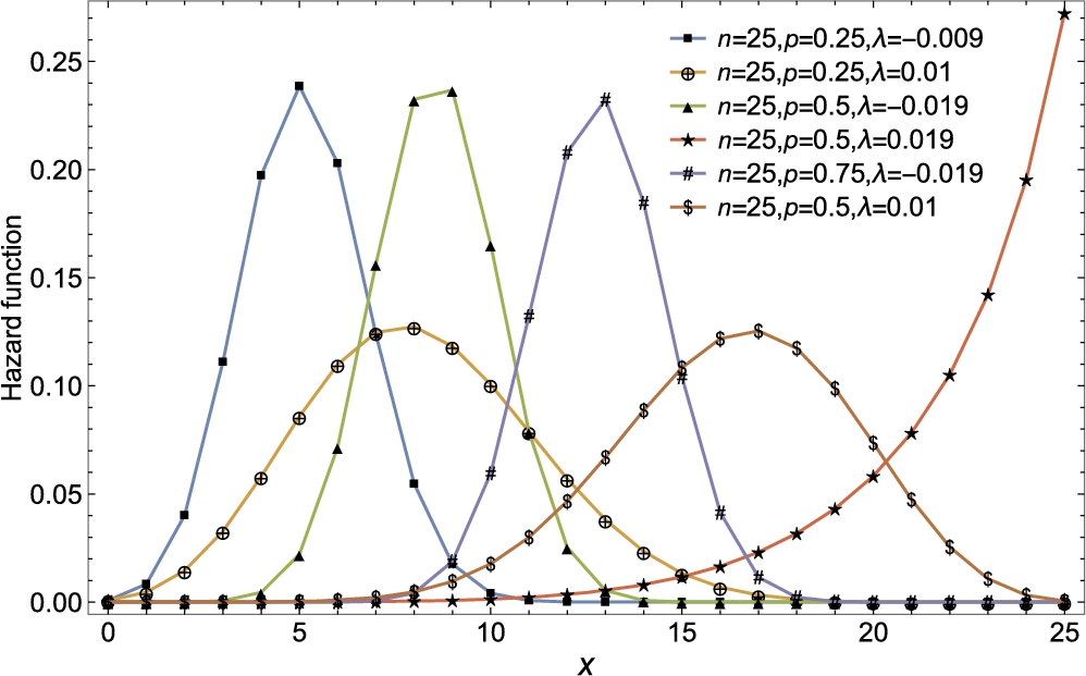
The probability mass function and the hazard rate function of the family are presented in Figs 3.2 and 3.3 respectively.

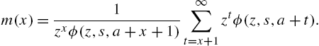
To simplify (3.33) further, we apply (Magnus et al., 1966)

to write a closed-form expression
The mean residual life is given by
It now follows that
or
Lerch family can be written in the form (3.20) with
as a modified power series family with parameter z in place of ![]() . Hence, the moments satisfy the recurrence formula
. Hence, the moments satisfy the recurrence formula
for the central moments, and
connecting the factorial moments. With the use of the expressions for μ and ![]() given above, the central and factorial moments can be computed. In the context of reliability modelling, the following characterization in terms of reliability concepts are useful.
given above, the central and factorial moments can be computed. In the context of reliability modelling, the following characterization in terms of reliability concepts are useful.
Theorem 3.2
Proof
We have
Differentiating with respect to z, we get

and so

By virtue of the identity

and the fact that
(3.38) simplifies to (3.37). To prove the sufficiency part, condition (3.7) means that

Changing ![]() to x and from the resulting equation, subtracting (3.39), yields
to x and from the resulting equation, subtracting (3.39), yields
or
Upon integrating, we get
Since ![]() and
and ![]() we have the proof. □
we have the proof. □
Theorem 3.3
Proof


Proof
Theorem 3.5

Proof
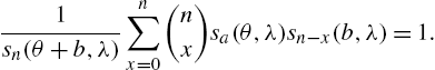
Sudheesh and Nair (2010) have characterized the modified power series family by

Since the Lerch family is a special case when ![]() , we have
, we have
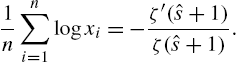
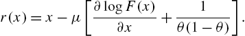
The estimation of parameters of the Lerch family has been addressed by Aksenov and Savageau (2005), who proposed the method of moments and the method of maximum likelihood. Denoting the sample moments by
from a random sample ![]() from the distribution, the equations to be solved in the method of moments are as follows:
from the distribution, the equations to be solved in the method of moments are as follows:

to get the estimates ![]() of
of ![]() . The above equations have to be solved numerically. Aksenov and Savageau (2005) also presented formulas for the asymptotic variances and covariances of the estimates obtained by the method of moments and the method of maximum likelihood.
. The above equations have to be solved numerically. Aksenov and Savageau (2005) also presented formulas for the asymptotic variances and covariances of the estimates obtained by the method of moments and the method of maximum likelihood.
Remark 3.2
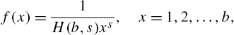
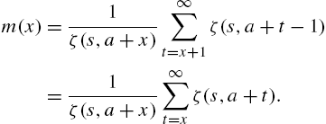
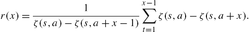
Gupta et al. (2008) have studied the Lerch family with positive integers as support. They considered the probability mass function of the form
where

The basic characteristics of this distribution are evaluated from

and
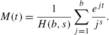
Other functions of interest are the probability generating function given by
the distribution function given by
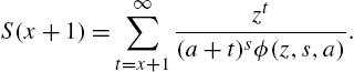
the survival function given by
the hazard rate given by
and the reversed hazard rate given by
The maximum likelihood method is proposed to estimate the parameters with the estimators solved from

and

They further observed that the likelihood equations are the same as the method of moments equations.
Zornig and Altmann (1995) and Kemp (2010) provided a list of members of the Lerch family. We now present some of these distributions and their properties. It may be noted that there is a difference in the expressions for the probability generating functions when the supports are different. For instance,

The geometric distribution is a member of all the families discussed so far, and hence enjoys the properties of all families. In addition to some of the characteristic properties already discussed in the preceding chapter, we present a few more results here that are relevant to reliability studies. The foremost among them is the no-ageing (lack of memory) property of the geometric lifetimes. It states that X is geometric with probability mass function
if and only if
for all
Writing (3.46) as
we can recognize the left hand side as the distribution of the residual life Being a characteristic property, for devices that does not age with time, the geometric law provides a suitable model. This is consistent with our earlier observation that the hazard rate, mean residual life and variance residual life are constant independent of the age of the device. Further, all these properties are equivalent to one another. The notion of no-ageing, also defined as
for all
in which case also the no-ageing property applies when X is replaced
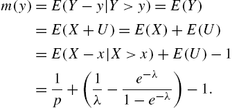
It is more informative to pursue the above results in a more general framework. Let Y be a continuous random variable with probability density function
Here, J stands for the absolute Jacobian of transformation and
Example Starting with the exponential case
which is again the exponential distribution truncated at unity. The application of the above result in reliability analysis is quite clear. On the one hand, we can convert the data on exponential to geometric and vice versa. Also by simulating exponential observations, their integer parts will be geometric. Some of the reliability functions from one distribution can be expressed in terms of the other. For example, in the exponential case, the mean residual life function is
Thus, the difference between the mean residual lives of the exponential and geometric lifetimes is
Theorem 3.7
Proof
The discrete uniform distribution arises from (3.30) when
It has distribution function
If
and
Among the reliability functions, the hazard rate is
a constant, characterizing the uniform distribution as a special case of the negative hypergeometric distribution (see Chapter 1). The variance residual life is found to be
Also, the functions in reversed time turns out to be
with their product
a constant. Further, the reversed variance residual life becomes
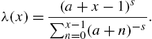
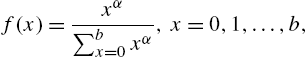
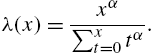
which is also a characterization of the discrete uniform distribution. The discrete Pareto distribution, also known as the Zipf distribution and as Riemann zeta distribution, is specified by the probability mass function (Fig. 3.4)
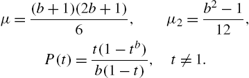
where
and
and the moments are infinite for
Some special cases of the discrete Pareto are the Estoup model, given by
(who noted that the rank r and frequency f in a French text were related by a hyperbolic law which translates in to the form (3.52)) and the Lotka law given by
where
which is a proper distribution with
and accordingly
The mean and variance are given by
and the moment generating function is given by
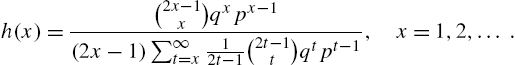
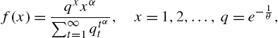
A distribution that is unrelated to the above, but bears the name ‘zeta distribution’ was introduced by Haight (1969) with probability mass function
The distribution and survival functions are, respectively,
and
Thus, the hazard and reversed hazard functions have simple closed form expressions as
and
Further, the mean residual life and reversed mean residual life are found to be
and
where
The variance of the distribution is
Notice that the mean is infinite for Figs 3.4–3.7 show hazard rate functions of discrete Pareto, Estoup, Lotka and truncated discrete Pareto distributions. A second major distribution belonging to the Lerch family is the Hurwitz-zeta distribution defined by
with
so that
Accordingly, the reliability functions have the expressions
Also,
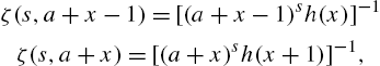
along with
leads to
Formula (3.55) enables the evaluation of successive hazard rates starting from
which leads to a compact expression of the form
Consequently, we have the recurrence relation
which can be determined iteratively by setting the initial value as
Hence,
By virtue of
we have a recurrence relation
The reversed mean residual life is given by
Further simplification yields
The probability mass function and hazard rate function of Hurwitz-zeta distribution are presented in Figs 3.8 and 3.9, respectively. A special case of the Hurtwitz-zeta model that is in use is the Zipf-Mandelbrot law (Mandelbrot, 1959, 1966) specified by
obtained when A third category of distribution in the Lerch family makes use of the general term in the polylogarithmic function Accordingly, the general form of the probability mass function in such cases is the Good distribution (Good, 1953) given by
with Setting
where
Historical remarks and the origin of the logarithmic series distribution and its properties can be found in Johnson et al. (1992). Regarding distributional properties, it may be noted that the probability generating function has the form
The factorial moment of order r is
from which the mean and variance are obtained as
Various central moments can be found from the above value of
From the recurrence relation for
with
giving
On the other hand, the hazard rate function is the reciprocal of an infinite series, viz.,
Hence,
Fig. 3.10 gives hazard rate functions of Good distribution. The rest of the reliability functions characterizing the logarithmic distribution are given in the following theorem.
Theorem 3.8
Proof
From (3.61), the mean residual life function of X is determined as
with the expression for Some general aspects of various distributions and their applications, other than those connected with reliability modelling, are given in the works of Vilaplana (1987), Gut (2005), Doray and Luong (1995, 1997), Kulasekera and Tonkyn (1992) and Panaretos (1989). Figs 3.1A, B, C and Fig. 3.3 provide the shapes of the hazard rate functions of the modified power series and Lerch families.Geometric Distribution
![]() , or equivalently,
, or equivalently,![]() . Thus, the residual life of a geometric lifetime at any age is the same as the original lifetime, thereby, justifying the name ‘no-ageing’ property.
. Thus, the residual life of a geometric lifetime at any age is the same as the original lifetime, thereby, justifying the name ‘no-ageing’ property.![]() , forms the basis of many ageing concepts discussed in the next chapter. Also, (3.47) suitably extended to higher dimensions is employed to generate various forms of multivariate geometric distributions; see Chapter 7 for details. A simple extension of the geometric law is possible by assuming X to take values
, forms the basis of many ageing concepts discussed in the next chapter. Also, (3.47) suitably extended to higher dimensions is employed to generate various forms of multivariate geometric distributions; see Chapter 7 for details. A simple extension of the geometric law is possible by assuming X to take values ![]() , with
, with![]() in (3.46). More interesting results of (3.48), in connection with ageing behaviour of X, can be seen in Chapter 4. Some additional properties of the geometric distribution are as follows:
in (3.46). More interesting results of (3.48), in connection with ageing behaviour of X, can be seen in Chapter 4. Some additional properties of the geometric distribution are as follows:
![]() are independent geometric random variables with parameter p, then
are independent geometric random variables with parameter p, then ![]() is distributed as negative binomial with parameters
is distributed as negative binomial with parameters ![]() ;
; ![]() are independent geometric random variables with parameters
are independent geometric random variables with parameters ![]() respectively, then
respectively, then ![]() is a geometric random variable with parameter
is a geometric random variable with parameter ![]() ;
;![]() and
and ![]() are independent random variables with same parameter p, then
are independent random variables with same parameter p, then ![]() has distribution
has distribution
![]() . Thus, geometric distribution arises as a mixture.
. Thus, geometric distribution arises as a mixture.
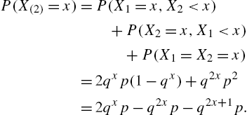
![]() ; see also Deng and Chhikkara (1990). Arising from the above result, it is also shown that the order statistics
; see also Deng and Chhikkara (1990). Arising from the above result, it is also shown that the order statistics ![]() ,
, ![]() , from the geometric distribution satisfies
, from the geometric distribution satisfies
![]() denotes equality in distribution, all variables on the right hand side are independent, and
denotes equality in distribution, all variables on the right hand side are independent, and ![]() as stated above. Also,
as stated above. Also,
![]() satisfying
satisfying ![]() , where D is an open subset of
, where D is an open subset of ![]() , the one-dimensional Euclidean space. If D can be divided into mutually exclusive regions
, the one-dimensional Euclidean space. If D can be divided into mutually exclusive regions ![]() with corresponding regions
with corresponding regions ![]() such that
such that ![]() ,
, ![]() , are injective and continuously differentiable. Then
, are injective and continuously differentiable. Then ![]() has probability density function
has probability density function![]() is the inverse of T (see Hoffman-Jorgensen, 1994). Applying the above transformation theorem with
is the inverse of T (see Hoffman-Jorgensen, 1994). Applying the above transformation theorem with ![]() ,
, ![]() ,
, ![]() , then
, then ![]() for every
for every ![]() . When Y is a continuous random variable with X as integer part and U as fractional part, we have the following result.
. When Y is a continuous random variable with X as integer part and U as fractional part, we have the following result.![]() . Even if failure times are observed at integer values, a very good approximation to continuous measurement can be made by virtue of the above result, from the estimated value of p, employing the equation
. Even if failure times are observed at integer values, a very good approximation to continuous measurement can be made by virtue of the above result, from the estimated value of p, employing the equation ![]() .
.
![]() and
and ![]() . The reliability properties follow from the general formulas for this family and also from our discussions in Chapter 2.
. The reliability properties follow from the general formulas for this family and also from our discussions in Chapter 2.Discrete Uniform Distribution
![]() ,
, ![]() and
and ![]() , with probability mass function
, with probability mass function![]() and survival function
and survival function ![]() . Various distributional characteristics are as follows:
. Various distributional characteristics are as follows:![]() are independent random variables with distribution in (3.50), then
are independent random variables with distribution in (3.50), then ![]() and
and ![]() ,
, ![]() have respective probability mass functions
have respective probability mass functions![]() and the mean residual life function is
and the mean residual life function is ![]() , giving
, givingDiscrete Pareto
![]() is the Riemann zeta function defined earlier in (3.27). As a model of random phenomenon, the distribution in (3.51) have been used in literature in different contexts. It is used to model the size or ranks of objects chosen randomly from certain type of populations, for example, the frequency of words in long sequences of text approximately obeys the discrete Pareto law. Zipf (1949) law states that out of a population of N elements, the frequency of elements of rank
is the Riemann zeta function defined earlier in (3.27). As a model of random phenomenon, the distribution in (3.51) have been used in literature in different contexts. It is used to model the size or ranks of objects chosen randomly from certain type of populations, for example, the frequency of words in long sequences of text approximately obeys the discrete Pareto law. Zipf (1949) law states that out of a population of N elements, the frequency of elements of rank ![]() is (3.51) and hence the name Zipf distribution, when used in linguistics. Seal (1947) has used it to model the number of insurance policies per individual, and as the distribution of surnames by Fox and Lasker (1983); see also Good (1953) and Haight (1966). Various distributional characteristics are obtained as special cases of the corresponding results of the Lerch family. In particular, moments of (3.51) are given by
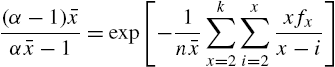
is (3.51) and hence the name Zipf distribution, when used in linguistics. Seal (1947) has used it to model the number of insurance policies per individual, and as the distribution of surnames by Fox and Lasker (1983); see also Good (1953) and Haight (1966). Various distributional characteristics are obtained as special cases of the corresponding results of the Lerch family. In particular, moments of (3.51) are given by![]() . The maximum likelihood estimator
. The maximum likelihood estimator ![]() is obtained by solving
is obtained by solving![]() . Lotka law results from the finding that the number of authors making n contributions is about
. Lotka law results from the finding that the number of authors making n contributions is about ![]() of those making one contribution, in which empirically a is nearly equal to two. When the value of x in (3.51) is truncated at b, we obtain
of those making one contribution, in which empirically a is nearly equal to two. When the value of x in (3.51) is truncated at b, we obtain![]() . In this case,
. In this case,![]() and
and ![]() is the mean.
is the mean.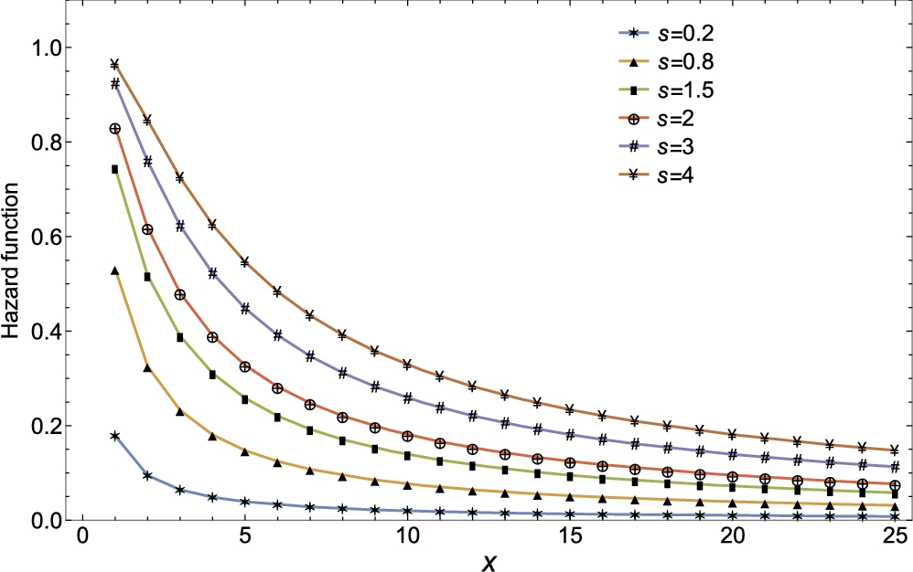
![]() and the variance is infinite for
and the variance is infinite for ![]() . Some further literature on discrete Pareto versions can be seen in Lin and Hu (2001) and Shan (2005).
. Some further literature on discrete Pareto versions can be seen in Lin and Hu (2001) and Shan (2005).


Hurwitz-Zeta Distribution
![]() being the Hurwitz-zeta function defined in (3.28). This distribution is mainly used in linguistics in connection with ranking problems. We note that
being the Hurwitz-zeta function defined in (3.28). This distribution is mainly used in linguistics in connection with ranking problems. We note that![]() . The expression for
. The expression for ![]() given above admits further simplification on applying the relationship
given above admits further simplification on applying the relationship![]() . We can write the mean residual life as
. We can write the mean residual life as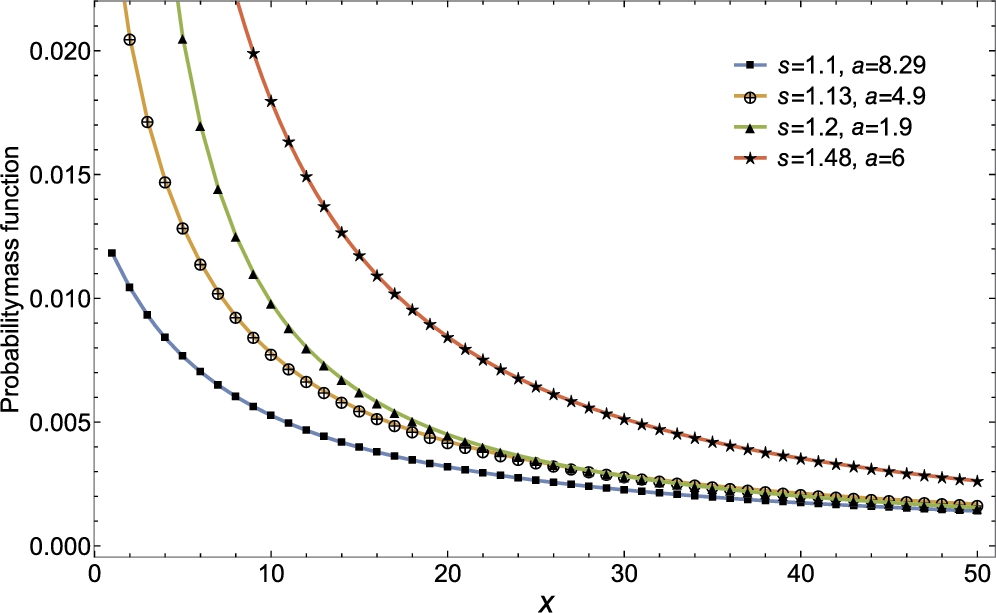

![]() in (3.54). See Zornig and Altmann (1995) for a discussion on the distribution.
in (3.54). See Zornig and Altmann (1995) for a discussion on the distribution.![]() defined in (3.29).
defined in (3.29).![]() . An important member in the above form, repeatedly used in the sequel, is the logarithmic series distribution (Fig. 3.8).
. An important member in the above form, repeatedly used in the sequel, is the logarithmic series distribution (Fig. 3.8).![]() in (3.57), we have the probability mass function of the distribution as
in (3.57), we have the probability mass function of the distribution as![]() . It is also member of the GPSD discussed above. It is easily seen that
. It is also member of the GPSD discussed above. It is easily seen that![]() and the recurrence relation
and the recurrence relation![]() mentioned in (3.58), the ratio
mentioned in (3.58), the ratio ![]() is always less than unity, so that
is always less than unity, so that ![]() is always a decreasing function. The distribution has a long tail and it resembles the geometric distribution for large values of x. We can identify the logarithmic series distribution by plotting
is always a decreasing function. The distribution has a long tail and it resembles the geometric distribution for large values of x. We can identify the logarithmic series distribution by plotting ![]() against x, where
against x, where ![]() is the observed frequency of x (see Eq. (3.58)). The plot is expected to give a straight line parallel to the x-axis with intercept z. In problems of estimation of z, the maximum likelihood estimator
is the observed frequency of x (see Eq. (3.58)). The plot is expected to give a straight line parallel to the x-axis with intercept z. In problems of estimation of z, the maximum likelihood estimator ![]() is obtained by solving the equation
is obtained by solving the equation![]() being the mean of a random sample drawn from the distribution. The reversed hazard rate function is
being the mean of a random sample drawn from the distribution. The reversed hazard rate function is
![]() given above.
given above.


3.2.4 Abel Series Distributions
The family of Abel series distributions is named after the Norwegian mathematician Niels Henrik Abel (1802–1829) who found the series whose general term specifies the probability mass function of the family. Abel polynomials (Comptet, 1994) are defined in terms of sequence ![]() , where
, where
with the first term ![]() and the second term
and the second term ![]() . Successive differentiation of (3.63) with respect to θ yields
. Successive differentiation of (3.63) with respect to θ yields
For a fixed λ, not related to θ, ![]() forms the basis of a set of polynomials in θ. Hence, for a finite, positive and successively differentiable function
forms the basis of a set of polynomials in θ. Hence, for a finite, positive and successively differentiable function ![]() in θ, we have
in θ, we have
where

Accordingly, restricting the parameter space to ![]() for which the terms in the expansion (3.65) are non-negative, we conclude that
for which the terms in the expansion (3.65) are non-negative, we conclude that
qualifies to be a probability mass function of a discrete random variable X. The distribution in (3.66) will be designated as the Abel series distribution (ASD), with series function ![]() . It may be noted that the truncated version of the ASD is also an ASD.
. It may be noted that the truncated version of the ASD is also an ASD.
Some special notation and functions are required to describe the properties of ASD, as given in Charalambides (1990). They are the shift operator E and the usual differential operator D combined to give
The Bell partition polynomials
are defined by

where the summation is extended over all partitions of n over ![]() satisfying
satisfying ![]() and
and ![]() is the number of parts of the partition. The special cases
is the number of parts of the partition. The special cases ![]() ,
, ![]() , and
, and ![]() ,
, ![]() , for real s of the Bell polynomials are denoted by
, for real s of the Bell polynomials are denoted by ![]() and
and ![]() . Also, let
. Also, let
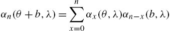
be the generating function of the sequence ![]() . With the above notations Charalambides (1990) has then shown that
. With the above notations Charalambides (1990) has then shown that
- (i) the probability generating function of ASD is
- where
 ,
,  is the inverse of q and
  ;
; - (ii) the factorial moments are given by
- with

- where
Various basic members of the ASD are obtained by the Abel series expansions of the exponential, binomial and logarithmic functions. We will discuss these distributions in some detail.
Generalized Poisson Distribution
Take
and consequently ![]() . Thus, we have the probability mass function as
. Thus, we have the probability mass function as

representing the generalized Poisson distribution of Consul and Jain (1973a, 1973b) who obtained it from the Lagrangian expansion. A comprehensive study of this distribution is available in Consul (1989). By way of properties of the distribution, we have:
and

where ![]() is
is ![]() with λ and θ replaced by λt and θt, respectively.
with λ and θ replaced by λt and θt, respectively.
The distribution in (3.67) is a modified power series distribution. We can estimate the parameters by the method of moments as

and
where ![]() and
and ![]() is the ith sample moment,
is the ith sample moment, ![]() .
.
Regarding reliability characteristics, which has not been studied so far, we first observe that the hazard rate function is

Also, (3.69) satisfies the relationship
from which successive values of ![]() can be calculated starting with
can be calculated starting with ![]() .
.
Secondly, the mean residual life function is obtained from the theorem due to Consul (1995) given below, with parametrization as ![]() .
.

Reliability functions in reversed time obey similar properties. We have
and therefrom
Differentiating the distribution function

and simplifying the resulting expression, we obtain

Thus, the reversed mean residual life has the expression
When ![]()
![]() , all the above results reduce to those of the Poisson distribution. In the Poisson process, the probability of occurrence of a single event remains constant, whereas in the generalized Poisson case the probability depends on the previous occurrence. On the basis of experimental evidence, the generalized case appears to model situations in which failures occur rarely in short periods of time where the frequency of such events are of interest over longer duration of time.
, all the above results reduce to those of the Poisson distribution. In the Poisson process, the probability of occurrence of a single event remains constant, whereas in the generalized Poisson case the probability depends on the previous occurrence. On the basis of experimental evidence, the generalized case appears to model situations in which failures occur rarely in short periods of time where the frequency of such events are of interest over longer duration of time.
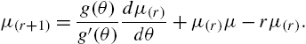
Quasi-Binomial Distribution I
Set ![]() ,
,
and

When ![]() , we have the probability mass function
, we have the probability mass function

A random variable X having its as probability mass function as in (3.71) is said to have a quasi-binomial distribution I (QBD-I). The probabilities of X are computed from the recurrence relation

QBD-I is unimodal and the values of the parameter λ substantially affects various characteristics of the distribution. Expressions for the mean and variance are

and

respectively. When ![]() , the mean of the QBD 1 is larger (smaller) than the mean of the binomial. Further distributional aspects and estimation of the parameters have been discussed by Consul and Famoye (2006).
, the mean of the QBD 1 is larger (smaller) than the mean of the binomial. Further distributional aspects and estimation of the parameters have been discussed by Consul and Famoye (2006).
The hazard rate function of QBD 1 is given by
and there exists a recurrence formula of the form

with ![]() . Likewise, the reversed hazard rate satisfies the recurrence formula
. Likewise, the reversed hazard rate satisfies the recurrence formula

with ![]() .
.
The probability mass functions and hazard rate functions of quasi-binomial distribution are presented in Figs 3.11 and 3.12, respectively.

Quasi-Negative Binomial Distribution
Taking ![]() , we have
, we have

Thus,

or

defines a probability distribution, which is called the quasi-negative binomial distribution (QNBD). In (3.74), ![]() ,
, ![]() and
and ![]() in the original expansion. Some special cases of (3.73) are as follows:
in the original expansion. Some special cases of (3.73) are as follows:
- (i) the negative binomial when
 ;
; - (ii) the quasi-geometric distribution (QGD)
- when
 and
and - (iii) the geometric distribution when and .
The probability mass function, for successive values of x, satisfies the recursive formula
and the moments are evaluated from the generating function
Eq. (3.74) yields the survival function as

From (3.74) and (3.75), we find that the hazard rate function can be computed from the recursive formula

Similarly, the reversed hazard rate function satisfies the recursive formula
When ![]() , we have the results for the quasi-geometric law. Models that lead to QNBD as well as various properties of QNBD have been discussed by Bilal and Hassan (2006) and Hassan and Bilal (2008). They have found the mean and variance to be
, we have the results for the quasi-geometric law. Models that lead to QNBD as well as various properties of QNBD have been discussed by Bilal and Hassan (2006) and Hassan and Bilal (2008). They have found the mean and variance to be
and

respectively, where
Quasi-Logarithmic Series Distribution
In this case, an extension of the usual logarithmic series distribution is obtained by taking ![]() . Then, the Abel series expansion yields
. Then, the Abel series expansion yields

so that

![]() , is a probability mass function, representing the quasi-logarithmic distribution. The hazard rate function becomes
, is a probability mass function, representing the quasi-logarithmic distribution. The hazard rate function becomes
Recurrence relations for ![]() and
and ![]() can be obtained in the usual manner. For instance, a recursive relation for the hazard function is given by
can be obtained in the usual manner. For instance, a recursive relation for the hazard function is given by

Quasi-Binomial Distribution II
The quasi-binomial distribution II (QBD II) can be derived in different ways. We obtain it here as a property of Abel polynomials and the corresponding series expansion. A sequence ![]() is of the binomial type if
is of the binomial type if
for all b. With the choice of
we have
from (3.64).
Hence,
Using the expansion in (3.66), we have
so that
Substituting for ![]() from (3.76), we see that
from (3.76), we see that
![]() ,
, ![]() ,
, ![]() and
and ![]() . The distribution defined by (3.77) is called QBD II. When
. The distribution defined by (3.77) is called QBD II. When ![]() , it reduces to the binomial model. A reparametrization of
, it reduces to the binomial model. A reparametrization of ![]() and
and ![]() provide another QBD II version
provide another QBD II version

The mean and variance of the form in (3.77) are
and

respectively. From (3.78), we can write expressions for the hazard rate and reversed hazard rate functions, respectively, as

and
They satisfy the recursive relationships
and
Figs 3.13 and 3.14 provide probability mass functions and hazard rate functions of quasi-binomial distribution II.

The Abel series distributions presented above have been obtained by Nandi and Das (1994). They have proposed estimates of the parameters of the distributions by equating the proportion of zeros and ones in the sample with ![]() and
and ![]() in the case of QBD I, QNBD and the generalized Poisson, and equating the sample mean and proportion of zeros with the population mean and
in the case of QBD I, QNBD and the generalized Poisson, and equating the sample mean and proportion of zeros with the population mean and ![]() for QBD II. With real data, it has also been shown that various distributions become useful in practice as satisfactory models. Chapter 4 of Consul and Famoye (2006) and the references therein provide more information on distributional properties, characterizations and application of the Abel series distributions in the general framework of Lagrangian expansions.
for QBD II. With real data, it has also been shown that various distributions become useful in practice as satisfactory models. Chapter 4 of Consul and Famoye (2006) and the references therein provide more information on distributional properties, characterizations and application of the Abel series distributions in the general framework of Lagrangian expansions.
3.2.5 Lagrangian Family
Consider a function ![]() which is successively differentiable satisfying
which is successively differentiable satisfying ![]() and
and ![]() . Then, the numerically smallest root
. Then, the numerically smallest root ![]() of the transformation
of the transformation ![]() defines a probability generating function with Lagrangian expansion
defines a probability generating function with Lagrangian expansion

provided that the derivative inside the square brackets is non-negative for all ![]() . The corresponding probability mass function is
. The corresponding probability mass function is

which constitutes the basic Lagrangian distributions. Detailed study of the properties, applications and estimation problems connected with this family is available in works of Mohanty (1966), Consul and Shenton (1972, 1973, 1975), and the books by Consul (1989) and Consul and Famoye (2006). We, therefore, represent here only these results that are most pertinent to reliability modelling and analysis. A large number of distributions belong to the Lagrangian family, of which we discuss only those for which the support is appropriate and where some useful and simple results on various reliability functions can be presented.
Chronologically, the earliest distribution is that of Borel specified by
By transferring the random variable X in (3.81) to ![]() , we have the generalized Poisson distribution presented earlier in (3.67). Since details of the Borel distribution can be evaluated in terms of these of the generalized Poisson, we abstain from further discussions here.
, we have the generalized Poisson distribution presented earlier in (3.67). Since details of the Borel distribution can be evaluated in terms of these of the generalized Poisson, we abstain from further discussions here.
Haight Distribution
The Haight (1961) distribution has probability mass function

From the probability generating function
the basic characteristics such as the mean, variance and higher moments can all be easily derived. The hazard rate function is
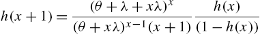
As usual, ![]() can be evaluated recursively as
can be evaluated recursively as
with ![]() . Differentiating the survival function
. Differentiating the survival function

with respect to p and rearranging the terms, we get

Accordingly, the mean residual life function is

Differentiating ![]() twice with respect to p, we get
twice with respect to p, we get

which leads to
and to

Now, the variance residual life can be computed from (3.84) and (3.86), as
With the aid of the distribution function

some similar manipulations yield reliability functions in reversed time. The expressions are

and
where
and

Geeta Distribution
A discrete random variable X is said to have Geeta distribution with parameters θ and α if
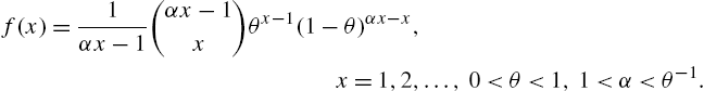
The distribution is L-shaped and unimodal with
and
A recurrence relation is satisfied by the central moments of the form
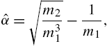
Estimation of the parameters can be done by the method of moments or by the maximum likelihood method. Moment estimates are
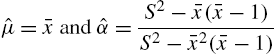
with ![]() and
and ![]() being the sample mean and variance. The maximum likelihood estimates are
being the sample mean and variance. The maximum likelihood estimates are
and ![]() is iteratively obtained by solving the equation
is iteratively obtained by solving the equation
with ![]() as the sample size and
as the sample size and ![]() is the frequency of
is the frequency of ![]() . For details, see Consul (1990). As the Geeta model is a member of the MPSD, the reliability properties can be readily obtained from those of the MPSD discussed in Section 3.2.2.
. For details, see Consul (1990). As the Geeta model is a member of the MPSD, the reliability properties can be readily obtained from those of the MPSD discussed in Section 3.2.2.
Generalized Geometric Distribution II
Famoye (1997) obtained the model

which is a generalization of the geometric distribution, as (3.87) becomes the geometric law when ![]() . It is obtained from the Lagrangian expansion of the generating function of the geometric distribution. The mean and variance are
. It is obtained from the Lagrangian expansion of the generating function of the geometric distribution. The mean and variance are
Other distributional properties are derived from the central moments that satisfy the recurrence formula
using the value of ![]() given above. For any given set of values of x, the hazard rate function satisfies from the recursive relationship
given above. For any given set of values of x, the hazard rate function satisfies from the recursive relationship

with ![]() . Working as in the earlier cases, the mean residual life satisfies the relationship
. Working as in the earlier cases, the mean residual life satisfies the relationship

Also,

Simplifying, we obtain

This, along with

gives an expression for the variance residual life. The reversed hazard rate is derived from the recurrence relation

By adopting calculations similar to those of the mean residual life, we have the reversed mean residual life as
Finally, the estimates of the parameters can be obtained by the moment method, or the maximum likelihood method, or by equating the sample mean and frequency at ![]() with the mean and
with the mean and ![]() , where n is the sample size.
, where n is the sample size.
There are several other families of discrete distributions discussed in the literature like the generalized hypergeometric family (Kemp, 1968a, 1968b), Gould series distributions (Charalambides, 1986), factorial series distributions (Berg, 1974) and their further extensions in various directions. Many of the members of these families overlap with those discussed here already. Furthermore, the reliability functions in other cases are of complicated forms, but can be obtained by some of the methods already detailed here.
3.3 Discrete Analogues of Continuous Distributions
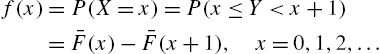
Several discrete distributions that are members of various families have been presented in the preceding section. They can serve as black-box models in the sense that their derivations were not based on the physical properties of the failure mechanism resulting in lifetimes. In a slightly different scenario, in this section, we consider various forms of discrete models that are obtained from popular continuous life distributions. This can be accomplished in different ways. Let Y be a continuous random variable representing lifetime with survival function ![]() . If times are grouped into unit intervals, the discrete variable
. If times are grouped into unit intervals, the discrete variable ![]() , the largest integer less than or equal to Y, has its probability mass function as
, the largest integer less than or equal to Y, has its probability mass function as
The survival function ![]() of X and
of X and ![]() of Y will be the same at all integer points. As a simple example, when Y is exponential with
of Y will be the same at all integer points. As a simple example, when Y is exponential with ![]() , we have
, we have

which represents the geometric distribution.
Discrete Weibull Distribution Taking ![]() and applying (3.88), we have
and applying (3.88), we have
This will be referred to as the discrete Weibull distribution I, first proposed by Nakagawa and Osaki (1975). For the model in (3.89), we readily find
and
The reversed hazard rate is

Two special cases of interest are the geometric when ![]() and the discrete Rayleigh when
and the discrete Rayleigh when ![]() . There are no closed-form expressions for the mean, variance, and higher-order moments. Alikhan et al. (1989) noted that
. There are no closed-form expressions for the mean, variance, and higher-order moments. Alikhan et al. (1989) noted that
and then proposed estimating the parameters q and β by equating the theoretical and estimated probabilities from the data of the observations ![]() and
and ![]() . Thus, these estimates are given by
. Thus, these estimates are given by

where ![]() is the empirical survival function. One can use two other values of X instead of 1 and 2, depending on the number of observations in the sample that are equal to the chosen integer values. The larger the frequencies of the numbers chosen, the better will be the estimates. Bracquemond and Gaudoin (2003) proposed the method of maximum likelihood for the estimation of q and β and observed that the estimates are biased, but of good quality for large values of q. One can use the distribution as an approximation to the continuous counterpart. Further, a shock model interpretation is also available, with X denoting the number of shocks survived by a device and q is the probability of surviving more than one shock. It can also be noted that (3.89) satisfies the extension of the lack of memory property that
is the empirical survival function. One can use two other values of X instead of 1 and 2, depending on the number of observations in the sample that are equal to the chosen integer values. The larger the frequencies of the numbers chosen, the better will be the estimates. Bracquemond and Gaudoin (2003) proposed the method of maximum likelihood for the estimation of q and β and observed that the estimates are biased, but of good quality for large values of q. One can use the distribution as an approximation to the continuous counterpart. Further, a shock model interpretation is also available, with X denoting the number of shocks survived by a device and q is the probability of surviving more than one shock. It can also be noted that (3.89) satisfies the extension of the lack of memory property that
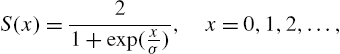
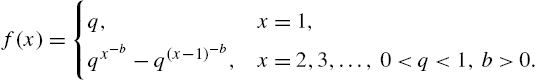
Discrete Half-Logistic Distribution The half-logistic model in the continuous case has survival function (Balakrishnan, 1985)

Accordingly, the discrete half-logistic distribution is specified by the survival function
or by the probability mass function

The mean and variance of the distribution in (3.90) are

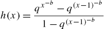
The hazard rate and reversed hazard rate functions of the distribution in (3.90) can be derived as follows:

There is only one parameter (σ) involved in (3.90) which can be estimated by the method of maximum likelihood.
Geometric Weibull Distribution This is a three-parameter model based on the continuous exponential Weibull distribution
introduced by Zacks (1984), where ![]() . Of the three parameters,
. Of the three parameters, ![]() represents scale,
represents scale, ![]() the shape and
the shape and ![]() is the change-point. The model was proposed in a practical situation when the hazard rate is constant until time a and thereafter it is increasing like a Weibull hazard rate. In the discrete analogue also, the same physical meaning prevails with
is the change-point. The model was proposed in a practical situation when the hazard rate is constant until time a and thereafter it is increasing like a Weibull hazard rate. In the discrete analogue also, the same physical meaning prevails with
and
We then have
as the hazard rate.
Telescopic Distributions A more general family of distributions result if we consider the discrete analogue of Y with survival function
when ![]() is a strictly increasing function with
is a strictly increasing function with ![]() and
and ![]() and
and ![]() . It includes the exponential, Rayleigh, Weibull, linear-exponential, and Gompertz distributions as special cases. Corresponding to
. It includes the exponential, Rayleigh, Weibull, linear-exponential, and Gompertz distributions as special cases. Corresponding to ![]() above, we have the distribution of X as
above, we have the distribution of X as
For the model in (3.92), it follows (Roknabadi et al., 2009) that

and the alternative hazard rate is
Discrete Inverse Weibull Distribution Jazi et al. (2010) considered the inverse Weibull law
to derive the discrete inverse Weibull distribution with survival function
and probability mass function
The distribution in (3.93) has decreasing ![]() for
for ![]() and unimodal with mode at 2, otherwise. When β becomes small, the tail becomes longer. The mean and variance do not have closed-form expressions. The hazard rate function and the alternative hazard rate function are, respectively,
and unimodal with mode at 2, otherwise. When β becomes small, the tail becomes longer. The mean and variance do not have closed-form expressions. The hazard rate function and the alternative hazard rate function are, respectively,
and

In order to estimate the parameters Jazi et al. (2010) considered the method of proportions, method of moments, a heuristic algorithm and an inverse Weibull probability plots. The discrete version of the probability plot is given by
which is a straight line and accordingly β and q can be estimated by a simple linear regression model fitted to the data.
Discrete Generalized Exponential Distribution Recalling that the generalized exponential distribution has its survival function as
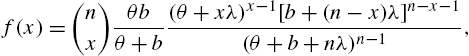
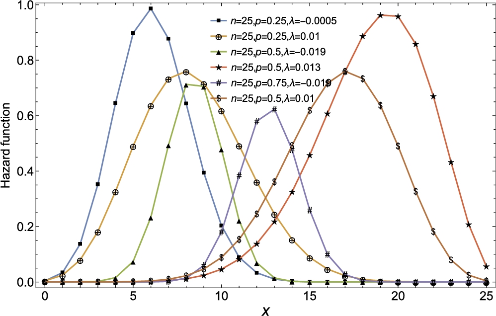
Nekoukhou et al. (2013) derived its discretized version as

with support ![]() . For integer values of α, the sum in (3.94) terminates at α. The distribution is unimodal for all α and p. There is a closed form expression for the moments given by
. For integer values of α, the sum in (3.94) terminates at α. The distribution is unimodal for all α and p. There is a closed form expression for the moments given by
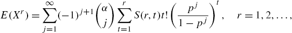
where

is the Stirling number of the second kind. In particular, we have
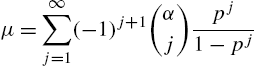
and

The parameters are estimated by the method of maximum likelihood by solving the equations

and

Using the survival function
we can write the hazard rate and reversed hazard rate functions as
and

The alternative hazard rate becomes

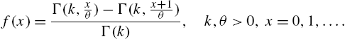
Discrete Gamma Distribution Chakraborty and Chakravarty (2012) considered the well-known two-parameter gamma distribution with survival function
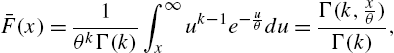
where
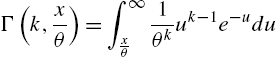
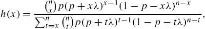
is the upper incomplete gamma function, to derive the discrete gamma model with probability mass function
As particular cases, we have the one-parameter discrete gamma when ![]() and the geometric when
and the geometric when ![]() ,
, ![]() . The distributional characteristics can be ascertained from the moments satisfying the recursive formula
. The distributional characteristics can be ascertained from the moments satisfying the recursive formula

where
In particular, we have
and
From a random sample of failure times ![]() , estimates of θ and k can be obtained by solving the likelihood equations
, estimates of θ and k can be obtained by solving the likelihood equations

and

with ![]() , being the digamma function.
, being the digamma function.
The reliability functions of interest are the survival function

the hazard rate function

the alternative hazard rate function
and the reversed hazard rate function
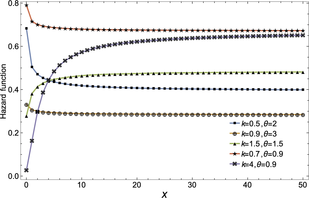
The hazard rate functions of discrete gamma distribution are presented in Fig. 3.15.
Discrete Lindley Distribution The Lindley distribution, in the continuous case, has its survival function as

Accordingly, the discrete version takes on the form

and ![]() . From the probability generating function
. From the probability generating function

it is easy to obtain
and

We also have


so that

and

Fig. 3.16 presents hazard rate functions of discrete Lindley distribution.

The maximum likelihood estimate of λ can be obtained as the solution of the equation

where ![]() is the mean of a random sample of size n from the discrete Lindley distribution.
is the mean of a random sample of size n from the discrete Lindley distribution.
Besides the above results on the discrete Lindley distribution described in Gomez-Deniz and Calderin-Ojeda (2011), there are some other results on the reliability characteristics. We note that

Hence, the mean residual life function can be expressed in a simple form as

which is a homographic function of x. Moreover, as a corollary to Eq. (3.9) characterizing the Ord family, we have the following theorem.
Theorem 3.10
Unlike in the case of most discrete models, the variance residual life has also a closed-form expression given by

with ![]() as given in (3.101).
as given in (3.101).
The reversed mean residual life has the expression

A characterization of the distribution by relationship between ![]() and
and ![]() can be derived along the lines of Theorem 3.3.
can be derived along the lines of Theorem 3.3.
Theorem 3.11
Further, the odds functions are
and ![]() .
.
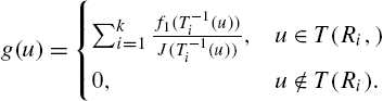
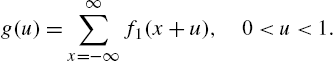
A second approach to construct discrete analogues of continuous distributions is to use the formula

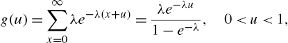
where ![]() is the probability density function of a continuous random variable. When
is the probability density function of a continuous random variable. When ![]() , for example, (3.103) results in
, for example, (3.103) results in
the Good distribution in (3.57). For a detail study of this distribution, we refer to Kulasekera and Tonkyn (1992). Obviously, the geometric distribution can also be derived from the exponential density function in this manner. See Sato et al. (1999) for an application of such a model, and also the convolution of their discrete exponential in the form of a negative binomial law. Lai and Wang (1995) obtained an analogue of the power distribution with density function
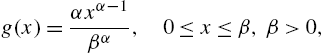
in the form
with hazard rate

and reversed hazard rte
Lai (2013) has also suggested construction of new models by discretizing the continuous hazard rate function or the alternative hazard rate function. Further discussion on the above methods and models derived therefrom can be seen in Kemp (2008) and Krishna and Pundir (2009).
3.4 Some Other Models
In this section, we present some other models arising from a variety of considerations.
Discrete Weibull Distribution II Stein and Dattero (1984) introduced a second form of Weibull distribution by specifying its hazard rate function as

The probability mass function and survival function are derived from ![]() using the formulas in Chapter 2 to be
using the formulas in Chapter 2 to be

and
By comparison, the discrete Weibull I has survival function of the same form as the continuous counterpart, while discrete Weibull II has the same form for the hazard rate function. Stein and Dattero (1984) have pointed out that a series system with two components that are independent and identically distributed have a distribution of the form in (3.104).
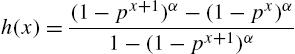
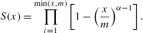
Discrete Weibull Distribution III A third type of Weibull distribution proposed by Padgett and Spurrier (1985) is specified by

with
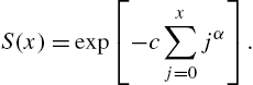
Accordingly, the hazard function is
For ![]() , (3.105) reduces to the geometric case. An important advantage of this model is that the hazard rate is flexible, in the sense that it can assume different shapes. In view of the complex nature of the probability mass function, the maximum likelihood estimates becomes computationally tedious and intensive. Bracquemond and Gaudoin (2003) have pointed out that the quality of the maximum likelihood estimate of c, as regards bias, increases with c, while the bias for α is small except for very small samples.
, (3.105) reduces to the geometric case. An important advantage of this model is that the hazard rate is flexible, in the sense that it can assume different shapes. In view of the complex nature of the probability mass function, the maximum likelihood estimates becomes computationally tedious and intensive. Bracquemond and Gaudoin (2003) have pointed out that the quality of the maximum likelihood estimate of c, as regards bias, increases with c, while the bias for α is small except for very small samples.
“S” Distribution Bracquemond and Gaudoin (2003) derived the “S” distribution based on some physical characteristics of the failure pattern through a shock-model interpretation. They have assumed a system in which on each demand a shock can occur with probability p and not occur with probability ![]() . The number of shocks
. The number of shocks ![]() at the xth demand is such that the hazard rate is an increasing function of
at the xth demand is such that the hazard rate is an increasing function of ![]() satisfying
satisfying
Then, the survival function, given ![]() , is
, is

Further, if ![]() , the
, the ![]() 's are independent Bernoulli (p) random variables, so that
's are independent Bernoulli (p) random variables, so that
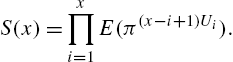
This leads to the “S” distribution specified by the probability mass function

and the survival function
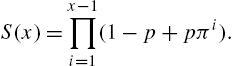
The interpretation given to the parameters is that p is the probability of a shock and π is the probability of surviving such a shock. We then have
Various properties of the distribution as well as the estimation issues have not been studied yet.
There are two other distributions proposed by Salvia and Bollinger (1982) and their generalizations by Padgett and Spurrier (1985), which are essentially particular cases of the models already discussed. Alzaatreh et al. (2012) provided a general method for deriving new distributions from continuous or discrete models. Let ![]() be the distribution function of a random variable Y which may be continuous or discrete and
be the distribution function of a random variable Y which may be continuous or discrete and ![]() be the probability density function of a continuous random variable T taking values in
be the probability density function of a continuous random variable T taking values in ![]() . Then, a new distribution can be defined by the distribution function
. Then, a new distribution can be defined by the distribution function

where ![]() is the distribution function of T. When Y is discrete, the new distribution has probability mass function
is the distribution function of T. When Y is discrete, the new distribution has probability mass function
For instance, when X has a geometric (p) distribution, the corresponding distribution arising from a continuous distribution with ![]() as the distribution function is
as the distribution function is
where ![]() . Another category of models arise when they are required to satisfy certain specific properties for their reliability characteristics, such as bathtub shaped hazard rate functions. Such distributions will be taken up later on in Chapter 5. Expressions for hazard rate function for some distributions are presented in Table 3.2 for ease reference.
. Another category of models arise when they are required to satisfy certain specific properties for their reliability characteristics, such as bathtub shaped hazard rate functions. Such distributions will be taken up later on in Chapter 5. Expressions for hazard rate function for some distributions are presented in Table 3.2 for ease reference.
Table 3.2
| Distribution |
|
|
|---|---|---|
| binomial |
|
|
| Poisson |
|
|
| negative binomial |
|
|
| Haight zeta | (2x−1)−σ − (2x+1)−σ | |
| geometric | q x p | p |
| Waring |
|
|
| negative hypergeometric |
|
|
| uniform |
|
|
| arithmetic |
|
|
| S |
|
p(1 − πx) |
| Weibull I |
|
|
| Weibull II |
|
|
| Weibull III |
|
|
| power |
|
|
| Lindley |
|
|
| gamma |
|
|
| quasi binomial II |
|
|
| quasi logarithmic |
|
|
| generalized Poisson |
|
|
| Hurtwitz-zeta |
|
|
| Lerch |
|
|
| linear hazard rate |
|
a + bx |