
Basic Reliability Concepts
Abstract
The basic reliability functions that can be used to model lifetime data and explain the failure patterns are the topics of discussion in this chapter. We begin with the conventional hazard rate defined as the ratio of the probability mass function to the survival function. This is followed up by an alternative hazard function introduced to overcome certain limitations of the conventional rate. Properties of both these hazard rates and their interrelationships are discussed. Then, the concept of residual life distribution and its characteristics like the mean, variance and moments are discussed. Various identities connecting the hazard rates, mean residual life function and various residual functions are derived, and some special relationships are employed for characterizing discrete life distributions. We then work out two problems to demonstrate how the characteristic properties enable the identification of the life distribution. Also, the role of partial moments in the context of reliability modelling is examined. Various concepts in reversed time has been of interest in reliability and related areas. Accordingly, reversed hazard rate, reversed residual mean life and reversed variance life are all defined and their interrelationships and characterizations based on them are reviewed. In the case of finite range distributions, it is shown that all the concepts in reversed time can assume constant values and these are related to the reversed lack of memory property characteristic of the reversed geometric law. Along with the traditional reliability functions, the notion of odds functions can also play a role in reliability modelling and analysis. We explain the relevant results in this connection. The log-odds functions and rates and their applications are also studied. Mixture distributions and weighted distributions also appear as models in certain situations, and the hazard rates and reversed hazard rates for these two cases are derived and are subsequently used to characterize certain lifetime distributions.
Keywords
Hazard rate; Mean residual life; Partial moments; Concepts in reversed time; Odds function; Log odds rate characterizations
2.1 Introduction
As mentioned in the last chapter, the reliability of a device is the probability that the device performs its intended function for a given period of time under conditions specified for its operation. When the device does not perform its function satisfactorily, we say that it has failed. When the random variable X represents the lifetime of a device, the observation on X is realized as the time of failure. The primary concern in reliability theory is then to understand the pattern in which failures occur for different devices and under varying operating environments. This is often done by analyzing the observed failure times or ages at failure with the help of a model that satisfactorily represents the predominant features of the data. One direct method is to find a probability distribution that provides a reasonable fit to the observations. Sometimes, there may exist more than one distribution that can pass an appropriate goodness-of-fit test. In any case, it is more desirable to find a probability model that manifests certain physical properties of the failure mechanism. In reliability theory, some basic concepts that help in the study of failure patterns have been developed. The objective of this chapter is to define such concepts and discuss their properties and inter-relationships. Two important aspects that necessitate the study of these concepts are (a) various functions considered in this context determine the life distribution uniquely, so that the knowledge of their functional form is equivalent to that of the distribution itself, and (b) it should be easier to deal with these functions than the distribution function or probability density function of the corresponding distributions.
2.2 Hazard Rate Function
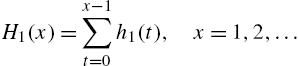
Let X be a discrete random variable assuming values in ![]() with probability mass function
with probability mass function ![]() and survival function
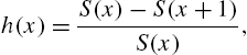
and survival function ![]() . We will think of X as the random lifetime of a device that can fail only at times (ages) in N. The hazard rate function of X is defined as
. We will think of X as the random lifetime of a device that can fail only at times (ages) in N. The hazard rate function of X is defined as
at points x for which ![]() . Treated as a function of x, the hazard rate is also called failure rate, instantaneous death rate, force of mortality and intensity function in other disciplines such as survival analysis, actuarial science, demography, extreme value theory and bio-sciences. Although in the continuous case, the concept of hazard rate dates back to historical studies in human mortality, its discrete version came up much later in the works of Barlow and Proschan (1965), Cox (1972) and Kalbfleisch and Prentice (2002), to mention a few.
. Treated as a function of x, the hazard rate is also called failure rate, instantaneous death rate, force of mortality and intensity function in other disciplines such as survival analysis, actuarial science, demography, extreme value theory and bio-sciences. Although in the continuous case, the concept of hazard rate dates back to historical studies in human mortality, its discrete version came up much later in the works of Barlow and Proschan (1965), Cox (1972) and Kalbfleisch and Prentice (2002), to mention a few.
When X has a finite support ![]() ,
, ![]() , then
, then ![]() . As a convention we take
. As a convention we take ![]() for
for ![]() . The hazard function
. The hazard function ![]() is interpreted as the conditional probability of the failure of the device at age x, given that it did not fail before age x. Thus,
is interpreted as the conditional probability of the failure of the device at age x, given that it did not fail before age x. Thus, ![]() . The interpretation and boundedness of the discrete hazard rate is thus different from that of the continuous case.
. The interpretation and boundedness of the discrete hazard rate is thus different from that of the continuous case.
We see from (2.1) that ![]() is determined from
is determined from ![]() or
or ![]() . The converse that the hazard rate function determines the distribution of X uniquely is also true. To see this, we note that
. The converse that the hazard rate function determines the distribution of X uniquely is also true. To see this, we note that
or
So,

Eq. (2.2) reveals also that ![]() can be used as a tool to model the life distribution. When a functional form for
can be used as a tool to model the life distribution. When a functional form for ![]() is assumed as model for a given data set, one has to ensure that the assumed form conforms to the hazard rate function of a distribution. The following theorem is useful in this regard.
is assumed as model for a given data set, one has to ensure that the assumed form conforms to the hazard rate function of a distribution. The following theorem is useful in this regard.
Theorem 2.1
A necessary and sufficient condition that ![]() is the hazard rate function of a distribution with support N is that
is the hazard rate function of a distribution with support N is that ![]() for
for ![]() and
and ![]() .
.
If the probability mass function is required from (2.1) and (2.2), we see that

The above results have appeared repeatedly in several papers; see, for example, Gupta (1979), Shaked et al. (1995) and Kemp (2004).
Example 2.1
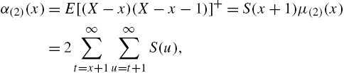
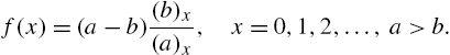
Example 2.2
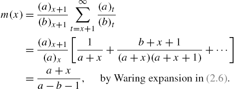
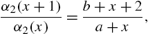
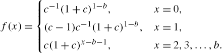
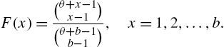
Consider the Waring distribution with parameters a and b (![]() ) having probability mass function
) having probability mass function

developed by Irwin (1968, 1975a, 1975b, 1975c), where
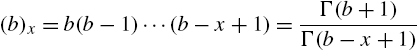
is the Pochammer's symbol. In studying the properties of this distribution, we need the Waring expansion
which converges for ![]() . Then,
. Then,

Hence, we get in this case
Example 2.3
A special case of the negative hyper geometric law with parameters n and k is defined by the probability mass function
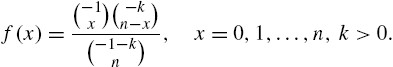
Then,

on using the identity
So,

Now to find the sum on the right hand side, the combinatorial expression (Riordan, 1968)

is employed in order to obtain
We then find

The distribution in (2.11) will be denoted by NH ![]() . For more functional forms of
. For more functional forms of ![]() that characterize various distributions, see Table 3.2.
that characterize various distributions, see Table 3.2.
Remark 2.1
The geometric, Waring and negative hyper-geometric models form a set of models possessing some attractive properties for their reliability characteristics, in as much the same way as the exponential, Pareto II and rescaled beta distributions in the continuous case. The results in the above examples show that the models (2.4), (2.5) and (2.8) have hazard rates of the form
with ![]() for geometric,
for geometric, ![]() for Waring, and
for Waring, and ![]() for negative hyper-geometric distributions.
for negative hyper-geometric distributions.
Remark 2.3
When Remark 2.1 is employed in a practical problem, it should be borne in mind that the support of X is N. Thus, the geometric distribution has a constant hazard rate means that a device with such a lifetime distribution does not age. However, when the support of X is ![]() ,
, ![]() leads to
leads to
If X has bounded support (![]() ), (2.12) is satisfied with
), (2.12) is satisfied with ![]() , then
, then ![]() and
and ![]() and
and ![]() . This follows from the facts that at
. This follows from the facts that at ![]() ,
, ![]() and at
and at ![]() ,
, ![]() .
.
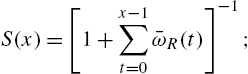
The sum of the hazard rates from 0 through ![]() is of interest in reliability theory and is called the cumulative hazard rate, defined by
is of interest in reliability theory and is called the cumulative hazard rate, defined by
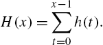
Also define ![]() . Graphically, the cumulative hazard rate represents the area under the step function representing
. Graphically, the cumulative hazard rate represents the area under the step function representing ![]() . Definition (2.13) does not satisfy properties analogous to the continuous case in which the cumulative hazard rate satisfies the identity
. Definition (2.13) does not satisfy properties analogous to the continuous case in which the cumulative hazard rate satisfies the identity
Therefore, Cox and Oakes (1984) proposed an alternative definition of cumulative hazard rate in the form
This means that

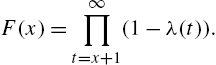
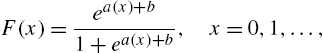
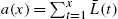
If
then ![]() is a cumulative hazard rate corresponding to an alternative hazard rate function defined by
is a cumulative hazard rate corresponding to an alternative hazard rate function defined by
Xie et al. (2002a) advocated the use of (2.17) as the hazard rate function instead of (2.1) by citing the following arguments. In the continuous case, the hazard rate is not a probability, but (2.1) is a conditional probability which is bounded. Consequently, (2.1) cannot increase too fast either linearly or exponentially to provide models of lifetimes of components in the wear-out phase. When cumulative hazard rate is defined as the negative logarithm of the survival function, ![]() . This causes problems in defining discrete ageing concepts that are analogues of their continuous counterparts, such as increasing hazard rate average (see Chapter 4). Thus, discrete ageing concepts based on
. This causes problems in defining discrete ageing concepts that are analogues of their continuous counterparts, such as increasing hazard rate average (see Chapter 4). Thus, discrete ageing concepts based on ![]() may not convey the same meaning as those in the continuous case. Similar problems persist with the construction of proportional hazards models and with series systems. Further details about these are provided in Sections 2.10 and 2.11. It may also be noted that unlike
may not convey the same meaning as those in the continuous case. Similar problems persist with the construction of proportional hazards models and with series systems. Further details about these are provided in Sections 2.10 and 2.11. It may also be noted that unlike ![]() , the definition of
, the definition of ![]() does not have any interpretation. Xie et al. (2002a) and Kemp (2004) have obtained the following interrelationships among the two hazard rate functions and the other reliability functions discussed so far:
does not have any interpretation. Xie et al. (2002a) and Kemp (2004) have obtained the following interrelationships among the two hazard rate functions and the other reliability functions discussed so far:
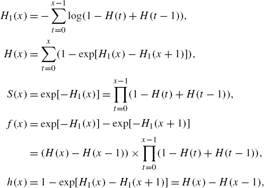
and
Thus, the function ![]() determines
determines ![]() uniquely and hence is useful in characterizing life distributions. We give some examples that compare the expressions of
uniquely and hence is useful in characterizing life distributions. We give some examples that compare the expressions of ![]() and
and ![]() .
.
Example 2.5
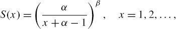
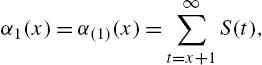
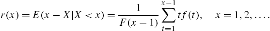
2.3 Mean Residual Life
The analysis of the lifetime of a device after it has attained age x is of special relevance in reliability and survival analysis. Thus, if X is the original lifetime with survival function ![]() , the corresponding residual lifetime after age x is the random variable
, the corresponding residual lifetime after age x is the random variable ![]() . From the definition of conditional probability, one can arrive at the distribution of
. From the definition of conditional probability, one can arrive at the distribution of ![]() as
as
The mean, variance, partial moments, coefficient of variation and percentiles of the distribution in (2.19) have been discussed extensively in the literature in the continuous case.
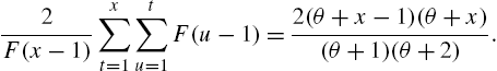
The mean residual life of X is defined as

It is easy to see that ![]() is the mean of the distribution in (2.19). When
is the mean of the distribution in (2.19). When ![]() ,
,

Characterizations of the distribution of X in terms of ![]() and the hazard rate have been studied by Nair and Hitha (1989). From (2.20),
and the hazard rate have been studied by Nair and Hitha (1989). From (2.20),
which leads to
and to the identity
Now, from (2.2), we have

Thus, the three functions ![]() ,
, ![]() and
and ![]() determine each other uniquely. Though
determine each other uniquely. Though ![]() can be determined from
can be determined from ![]() and vice-versa, both have unique features that ensure their necessity in reliability theory. The mean residual life function may exist when the hazard function does not exist and vice-versa, as will be seen in some of the examples that are considered later. While
and vice-versa, both have unique features that ensure their necessity in reliability theory. The mean residual life function may exist when the hazard function does not exist and vice-versa, as will be seen in some of the examples that are considered later. While ![]() is a local measure of failure patterns for any x, the mean residual life function depends upon the life history of devices at all ages beyond x and hence the latter is more informative. At the same time,
is a local measure of failure patterns for any x, the mean residual life function depends upon the life history of devices at all ages beyond x and hence the latter is more informative. At the same time, ![]() as a summary measure is highly sensitive to a single long-term survivor in a data set, which is not desirable. There are other interesting properties that distinguish the two concepts as will be seen in the subsequent chapters.
as a summary measure is highly sensitive to a single long-term survivor in a data set, which is not desirable. There are other interesting properties that distinguish the two concepts as will be seen in the subsequent chapters.
Since ![]() , we can note from (2.21) that
, we can note from (2.21) that
and ![]() . For many discrete distributions, the expression for
. For many discrete distributions, the expression for ![]() is not of a simple form. In the following examples, we have simple forms for
is not of a simple form. In the following examples, we have simple forms for ![]() that have many desirable properties. For more examples of the
that have many desirable properties. For more examples of the ![]() function, see Table 2.4.
function, see Table 2.4.
Example 2.6
For the geometric distribution ![]() in Example 2.1,
in Example 2.1,

is the reciprocal of the hazard rate function so that ![]() .
.
Example 2.7
The Waring distribution ![]() in Example 2.2 yields
in Example 2.2 yields
Notice that ![]() is a linearly increasing function and satisfies
is a linearly increasing function and satisfies ![]() .
.
Example 2.8

We can see that ![]() is linear and decreasing in x and
is linear and decreasing in x and ![]() .
.
Nair and Hitha (1989) and Hitha and Nair (1989) have established the following characterizations of the above three models.
Theorem 2.2
Theorem 2.3
Identification of lifetime distributions that are uniquely determined by simple relationships between various reliability concepts has attracted several studies in the past and continues to be a fertile area of research. Many results pertaining to individual distributions and families of distributions are available in this context. Theorem 2.3 belongs to this category concerning three specific distributions and its applications will be discussed later in Chapter 4. A more general result in this connection is the following.
Let ![]() and
and ![]() be real-valued functions defined on N such that
be real-valued functions defined on N such that ![]() and
and ![]() . We define
. We define
Further, assume that ![]() and
and ![]() , where Δ is the usual difference operator,
, where Δ is the usual difference operator, ![]() , and
, and ![]() is some real-valued function.
is some real-valued function.
Theorem 2.4
Let X be discrete random variable taking values in N and ![]() ,
, ![]() and
and ![]() be real-valued functions satisfying the above conditions. Then, for every
be real-valued functions satisfying the above conditions. Then, for every ![]() and some
and some ![]() and
and ![]() , the following statements are equivalent:
, the following statements are equivalent:
with ![]() and
and ![]() is evaluated from
is evaluated from ![]() ;
;
where ![]() in (2.25) is the hazard rate function.
in (2.25) is the hazard rate function.
When ![]() , we write
, we write
and call it the vitality function, which is in fact a conditional mean life function. It satisfies
Eq. (2.25) becomes a relationship between the mean residual life function and hazard rate function of the form
that characterizes the class of discrete distributions satisfying
where ![]() . It is further observed in Nair and Sudheesh (2008) that
. It is further observed in Nair and Sudheesh (2008) that
- (1) the equality in (2.26) holds if and only if
 is linear in
  ;
; - (2)
 ;
; - (3) the expression for
 is unique for a particular choice of , but one can have different choices for for the same distribution when is different;
 - (4) for a given , the corresponding characterizes the distribution of X.
Specialization of the identity in (2.25) for various distributions and their implications will be considered later in Chapter 3 wherein we discuss discrete lifetime models. The variance inequality is also useful in the unbiased estimation of functions of X.
Remark 2.4
Since ![]() , all the characteristic properties mentioned above can be translated in terms of
, all the characteristic properties mentioned above can be translated in terms of ![]() and
and ![]() .
.
Though closely related to the mean residual life function, the vitality function introduced in (2.28) has some importance in its own right in lifetime studies. By definition,
Some properties of ![]() that are of interest in the sequel are given below. From the definition
that are of interest in the sequel are given below. From the definition
Dividing by ![]() and simplifying, we get
and simplifying, we get
Further,
Analogous to the presentation on vitality function given in Kupka and Loo (1989), we note that in the integer interval ![]() ,
, ![]() represents the increment in the conditional mean life which is achieved by surviving from age 0 to x. Thus, low (high) values of
represents the increment in the conditional mean life which is achieved by surviving from age 0 to x. Thus, low (high) values of ![]() means that the device is ageing rapidly (slowly) during
means that the device is ageing rapidly (slowly) during ![]() and this justifies the name vitality function of the lifetime X. However, it may be noticed that vitality function is always non-decreasing, unlike the mean residual life function which can be either decreasing or increasing.
and this justifies the name vitality function of the lifetime X. However, it may be noticed that vitality function is always non-decreasing, unlike the mean residual life function which can be either decreasing or increasing.
Returning to the reliability functions based on real-valued functions ![]() of X, more characterizations and useful relationships can be seen. Let
of X, more characterizations and useful relationships can be seen. Let ![]() be the distribution function of X such that
be the distribution function of X such that ![]() for some
for some ![]() .
.
Theorem 2.5
Ruiz and Navarro (1995) considered discrete random variables taking values in ![]() ,
, ![]() , and defined for a monotonic
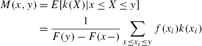
, and defined for a monotonic ![]() , the doubly truncated mean function
, the doubly truncated mean function
for ![]() ,
, ![]() and
and ![]() . Then,
. Then,
where

and
They also obtained a necessary and sufficient condition for a given function in ![]() to be a doubly truncated mean function. This result is of relevance in reliability modelling since
to be a doubly truncated mean function. This result is of relevance in reliability modelling since ![]() tends to the mean residual life as
tends to the mean residual life as ![]() and to the reversed mean residual life (Section 2.7) as
and to the reversed mean residual life (Section 2.7) as ![]() when
when ![]() and the range of X is N.
and the range of X is N.
The conditional moments

satisfy

so that the distribution of X is determined from ![]() by virtue of (2.2). Further, since the left hand side of (2.30) is independent of r,
by virtue of (2.2). Further, since the left hand side of (2.30) is independent of r,

is a recurrence relation connecting two consecutive moments.
Glanzel et al. (1984) considered ![]() to be a monotonic function such that
to be a monotonic function such that ![]() a constant in
a constant in ![]() for any finite n. Then,
for any finite n. Then,

Further, if ![]() and
and ![]() are two functions defined on N such that
are two functions defined on N such that ![]() is strictly monotonic, then the distribution of X has probability mass function
is strictly monotonic, then the distribution of X has probability mass function ![]() satisfying
satisfying
and ![]() . For a further refinement of the results on conditional expectations, see Su and Huang (2000). For characterizations of the geometric, Waring and negative hyper-geometric laws by doubly truncated mean residual life, one may see to Khorashadizadeh et al. (2012).
. For a further refinement of the results on conditional expectations, see Su and Huang (2000). For characterizations of the geometric, Waring and negative hyper-geometric laws by doubly truncated mean residual life, one may see to Khorashadizadeh et al. (2012).
The alternative hazard rate ![]() can also be related to
can also be related to ![]() , as shown in Xie et al. (2002a) when
, as shown in Xie et al. (2002a) when ![]() . From the definition of
. From the definition of ![]() in (2.19) and Eq. (2.2), we have
in (2.19) and Eq. (2.2), we have

Some relationships involving ![]() and
and ![]() needed in the subsequent discussions are
needed in the subsequent discussions are

and
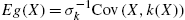
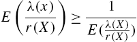
The expression ![]() is referred to as the hazard rate at random time. We now prove a characteristic property of the mean of
is referred to as the hazard rate at random time. We now prove a characteristic property of the mean of ![]() .
.

Proof
Consider
Applying the Cauchy-Schwarz inequality for real sequences ![]() and
and ![]() , viz.,
, viz.,
with ![]() and
and ![]() , we readily obtain
, we readily obtain

From (2.31), the inequality in (2.33) follows. The inequality in (2.34) becomes equality if and only if ![]() , in which case
, in which case ![]() ,
, ![]() , for all x. A constant hazard rate characterizes the geometric law. □
, for all x. A constant hazard rate characterizes the geometric law. □

Proof
Taking ![]() and
and ![]() and applying the Cauchy-Schwarz inequality, (2.35) follows. For the equality sign to hold,
and applying the Cauchy-Schwarz inequality, (2.35) follows. For the equality sign to hold, ![]() which implies
which implies ![]() , a characteristic property of the geometric distribution. □
, a characteristic property of the geometric distribution. □
Although we have defined the hazard rate function and the mean residual life function in terms of the time to failure of a device, the definitions and properties can also be used to model data on the time to occurrence of an ‘event’ with appropriate modifications in interpretations that best suit the context. Accordingly, the results mentioned so far have been extensively applied in other disciplines as well. A detailed examination of this aspect will be taken up later in Chapter 9. In the present section, we consider some real data and illustrate the application of the characterizations established above in finding suitable models for them.
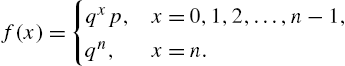
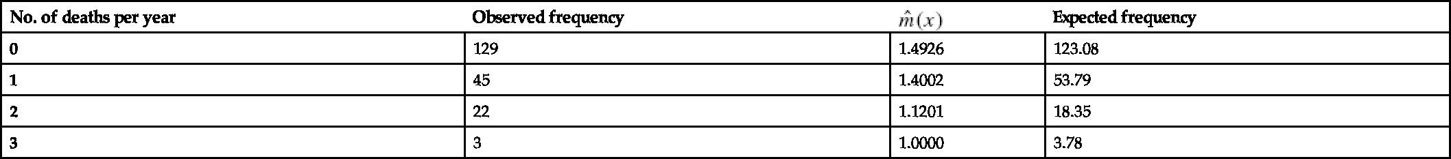
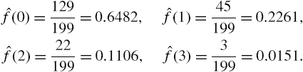
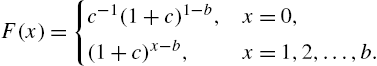
Example 2.11 In this example, we consider the famous Bortkiewicz data on the number of soldiers of the Prussian army who died of horse-kicks in a period of 20 consecutive years, with the modification of the data value suggested by Cohen (1960). The last observation in Cohen's data is omitted for the analysis; see Table 2.1 for details. From the data, the probability mass function of X, the time of death, is estimated as
Table 2.1 Model for the deaths of solders by horse-kicks
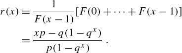
These values give the estimate of the mean residual life as
where
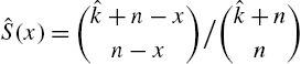
Being a linearly decreasing mean residual life, from Theorem 2.1, we propose the negative hyper-geometric distribution as a model for the data with
we obtain the estimate of k as
with
Obviously, the chosen model rests on the assumption of linearity of
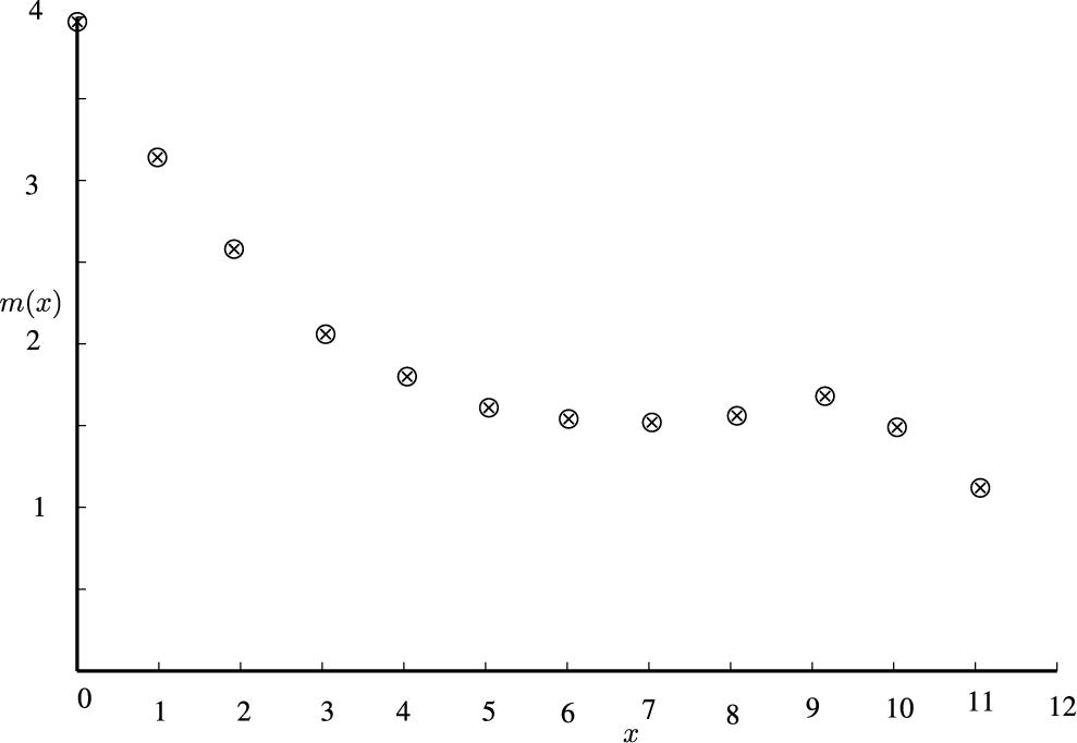
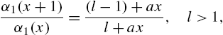
Example 2.12 The results of the well-known Rutherford-Geiger experiment is produced in Table 2.2. It describes the number of α-particles remitted from radioactive substances in 2608 fractions of 75 seconds. As in the previous example, the estimates Table 2.2 Estimated values of
We also have
so that an estimate of the mean becomes
Neither an examination of the values of
Hence, we can calculate
In (2.36), the estimate of the standard deviation σ is taken as the sample standard deviation. The values of
with Table 2.3 Goodness-of-fit for Rutherford-Geiger data
The chi-square value obtained above does not reject the hypothesis that the data follow the Poisson distribution. The following facts can be further observed:
2.3.1 Modelling Data
No. of deaths per year
Observed frequency
![]()
Expected frequency
0
129
1.4926
123.08
1
45
1.4002
53.79
2
22
1.1201
18.35
3
3
1.0000
3.78
![]() . The values of
. The values of ![]() can be seen in column 2 of Table 2.1. The next step is to seek a functional form for
can be seen in column 2 of Table 2.1. The next step is to seek a functional form for ![]() . Accordingly, a straight line fit is considered for
. Accordingly, a straight line fit is considered for ![]() by the method of least-squares. This yields
by the method of least-squares. This yields![]() . Comparing with the mean residual life function of the negative hyper-geometric law
. Comparing with the mean residual life function of the negative hyper-geometric law![]() . Thus the proposed model has survival function
. Thus the proposed model has survival function![]() and
and ![]() . The expected probability mass function is
. The expected probability mass function is![]() . Hence the model is validated by calculating the expected frequencies and then verifying their closeness by the chi-square goodness-of-fit test. The chi-square value of 2.4949 does not reject the model at 5% level of significance.
. Hence the model is validated by calculating the expected frequencies and then verifying their closeness by the chi-square goodness-of-fit test. The chi-square value of 2.4949 does not reject the model at 5% level of significance.![]() and
and ![]() of the probability mass function and the survival function and there from
of the probability mass function and the survival function and there from ![]() are found out. In addition, we also require the estimated hazard rate function
are found out. In addition, we also require the estimated hazard rate function ![]() . The observed values of
. The observed values of ![]() and
and ![]() are shown in Table 2.2.
are shown in Table 2.2.![]() ,
, ![]() and
and ![]() for the data in Table 2.3
for the data in Table 2.3
x
![]()
![]()
![]()
0
0.029
3.9569
2.00
1
0.0795
3.2124
2.06
2
0.1632
2.6437
2.07
3
0.2672
2.2431
1.96
4
0.3695
1.9716
1.87
5
0.4493
1.7642
1.85
6
0.5462
1.6839
1.65
7
0.6615
1.7604
1.61
8
0.5518
1.5576
2.81
9
0.6306
1.5082
2.01
10
0.6223
1.3478
2.23
11
0.6522
1.000
2.12
12
1.000

![]() and
and ![]() nor their plots in Figs 2.1 and 2.2 exhibit an obvious choice for the functional forms of
nor their plots in Figs 2.1 and 2.2 exhibit an obvious choice for the functional forms of ![]() and
and ![]() . In such cases, Theorem 2.4 can be of some assistance in the determination of a suitable model. Since we have the empirical mean residual life from the data, choose
. In such cases, Theorem 2.4 can be of some assistance in the determination of a suitable model. Since we have the empirical mean residual life from the data, choose ![]() so that (2.24) becomes
so that (2.24) becomes![]() from
from
![]() so arrived at are shown in Table 2.2. Notice that the value at
so arrived at are shown in Table 2.2. Notice that the value at ![]() is significantly larger than the rest. Barring this value, the rest appears to be clustering around the average
is significantly larger than the rest. Barring this value, the rest appears to be clustering around the average ![]() . This is the same as assuming
. This is the same as assuming ![]() , a constant for all x, since the least-square estimate of c is
, a constant for all x, since the least-square estimate of c is ![]() . Recall from Theorem 2.4 that the value of
. Recall from Theorem 2.4 that the value of ![]() uniquely determines the distribution of X and further,
uniquely determines the distribution of X and further, ![]() if and only if the distribution is Poisson with mean
if and only if the distribution is Poisson with mean ![]() . Thus, the data follows a Poisson distribution
. Thus, the data follows a Poisson distribution![]() . To validate the assumption made on
. To validate the assumption made on ![]() , we compare the observed and expected frequencies, when
, we compare the observed and expected frequencies, when ![]() , presented in Table 2.3.
, presented in Table 2.3.
x
Observed frequency
Expected frequency
Contribution to
![]() -value
-value
0
57
58.4
0.0036
1
203
221.7
1.5773
2
383
421.2
3.4644
3
525
533.6
0.1386
4
532
507.0
1.2327
5
408
385.2
1.3495
6
273
244.1
3.4215
7
139
132.5
0.3189
8
45
62.9
5.0934
9
27
26.6
0.0060
10
10
10.27
0.0039
![]()
![]() 6
64.4
0.5819
Total
2608
2608
16.2216
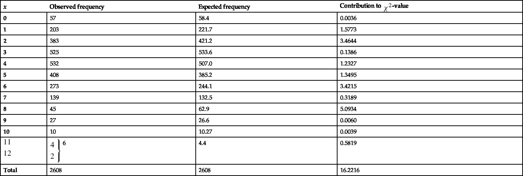
![]() is considerably larger compared to the rest. The plot of the hazard function shows that the function is decreasing markedly at this point which is uncharacteristic of the Poisson model where the hazard rate is increasing. If we use the maximum likelihood estimate
is considerably larger compared to the rest. The plot of the hazard function shows that the function is decreasing markedly at this point which is uncharacteristic of the Poisson model where the hazard rate is increasing. If we use the maximum likelihood estimate ![]() for the Poisson distribution, the difference is still higher with expected frequency 67. Thus, the
for the Poisson distribution, the difference is still higher with expected frequency 67. Thus, the ![]() value at
value at ![]() is taken as a discordant one and omitted in the calculation of
is taken as a discordant one and omitted in the calculation of ![]() .
.

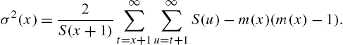
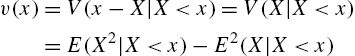
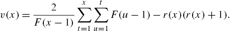
2.4 Variance Residual Life Function
The variance of the residual life ![]() is studied in reliability theory in various contexts. Primarily, its role is to define ageing concepts that are weaker than some ageing criteria based on the hazard rate and the mean residual life. Chapter 4 provides details in this direction. Secondly, variance of residual life has the same role as the usual variance when estimators of mean residual life are discussed. It is also required in the study of coefficient of variation of residual life. Assuming that
is studied in reliability theory in various contexts. Primarily, its role is to define ageing concepts that are weaker than some ageing criteria based on the hazard rate and the mean residual life. Chapter 4 provides details in this direction. Secondly, variance of residual life has the same role as the usual variance when estimators of mean residual life are discussed. It is also required in the study of coefficient of variation of residual life. Assuming that ![]() , we define the variance residual life function as
, we define the variance residual life function as
where ![]() is the mean residual life function defined in (2.20). Alternatively,
is the mean residual life function defined in (2.20). Alternatively,
The second factorial moment of the residual life ![]() , given by
, given by
will frequently appear in the sequel. We have the following expression for ![]() .
.
Proof

Hence,

which is equivalent to (2.39). Thus, the variance residual life function can be written in the form
An equivalent expression for (2.40), by defining the survival function as ![]() , has been obtained in Khorashadizadeh et al. (2010). □
, has been obtained in Khorashadizadeh et al. (2010). □
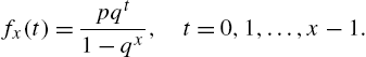
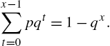
Example 2.13
For the geometric law considered in Example 2.6, we have
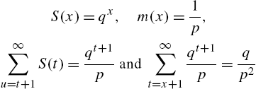
so that from (2.42), we have

which is the same as the variance of X.
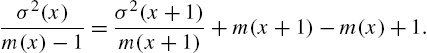
There exist some inter-relationships between the reliability functions discussed so far.
Proof
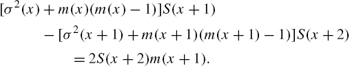
Remark 2.5
Proof


Unlike the cases of hazard rate and mean residual life functions, there is no inversion formula that expresses the survival function in terms of the variance residual life. Also, there are only a few standard distributions for which ![]() has simple tractable forms, as could be seen from Table 2.3. Therefore, characterizations of life distributions involving
has simple tractable forms, as could be seen from Table 2.3. Therefore, characterizations of life distributions involving ![]() take the form of its relationship with other concepts. Hitha and Nair (1989) have shown that
take the form of its relationship with other concepts. Hitha and Nair (1989) have shown that

if and only if X is geometric for ![]() , negative hyper-geometric for
, negative hyper-geometric for ![]() , and Waring for
, and Waring for ![]() . We also have a more general result satisfied by a class of distribution due to Sudheesh and Nair (2010). We retain the notations used for Theorem 2.4.
. We also have a more general result satisfied by a class of distribution due to Sudheesh and Nair (2010). We retain the notations used for Theorem 2.4.
Theorem 2.11
Let ![]() be a real-valued function of X that is non-decreasing and satisfying the following conditions:
be a real-valued function of X that is non-decreasing and satisfying the following conditions:
- (i)
 and
and  are finite;
 - (ii)
 and the support of X is an integer interval;
 - (iii)
 for all x.
Then, X has distribution specified by
for some real-valued function ![]() if and only if for all x
if and only if for all x

where ![]() stands for variance.
stands for variance.
Remark 2.7
Remark 2.8
2.5 Upper Partial Moments
A concept that is closely related to moments of residual life is that of partial moments, which can also be interpreted as moments of a different kind of residual life. The rth upper partial moment of X about a point x is defined as
where ![]() . In the case of discrete models, it is sometimes more convenient to work with factorial partial moments defined as
. In the case of discrete models, it is sometimes more convenient to work with factorial partial moments defined as
where
is the descending factorial expression. By virtue of the relationship

where ![]() is the Stirling number of the second kind,
is the Stirling number of the second kind, ![]() can be computed in terms of
can be computed in terms of ![]() . Nair et al. (2000) have studied several properties of
. Nair et al. (2000) have studied several properties of ![]() and their implications to reliability modelling. First, we note that
and their implications to reliability modelling. First, we note that
and hence
and
The upper partial moments satisfy the recurrence formula
Thus, any one partial moment sequence, particularly ![]() ,
, ![]() , determines all other partial moments. Since only the first two partial moments are of importance in reliability analysis we concentrate on their properties. Notice that
, determines all other partial moments. Since only the first two partial moments are of importance in reliability analysis we concentrate on their properties. Notice that
so that
and
From (2.51), the ratio of the upper partial means at consecutive values gives
Thus, from Theorem 2.2, we deduce the following result.
Theorem 2.12
The second factorial partial moment is
while
Thus, the variance residual life is calculated as

Then, from Example 2.2, we have

The ratios of partial moments admit simple forms in this case. For example,

and
both being homographic functions. A similar discussion of the properties is possible when the ascending factorial expression
is used instead of ![]() in (2.48); for details see Priya et al. (2000).
in (2.48); for details see Priya et al. (2000).
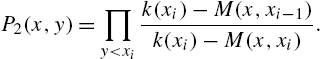
So far, we have considered reliability functions specified by the survival function ![]() . A parallel theory that builds up when the event
. A parallel theory that builds up when the event ![]() , defined by the distribution function, also has been of interest in reliability literature. Referred to by the name reliability functions in reversed time, they are found to be useful in modelling and analysis of lifetime data and also in other fields of study. We discuss some important functions in this category in the next few sections.
, defined by the distribution function, also has been of interest in reliability literature. Referred to by the name reliability functions in reversed time, they are found to be useful in modelling and analysis of lifetime data and also in other fields of study. We discuss some important functions in this category in the next few sections.
2.6 Reversed Hazard Rate
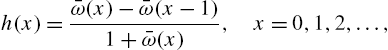
The reversed hazard rate of X is defined as
Thus, ![]() in the discrete case is interpreted as the conditional probability that a device fails at age x, given that its lifetime is at most x. Being a conditional probability,
in the discrete case is interpreted as the conditional probability that a device fails at age x, given that its lifetime is at most x. Being a conditional probability, ![]() . Keilson and Sumita (1982), who first defined the reversed hazard rate in continuous time, called it the dual failure function by the property that X has reversed hazard rate
. Keilson and Sumita (1982), who first defined the reversed hazard rate in continuous time, called it the dual failure function by the property that X has reversed hazard rate ![]() ,
, ![]() if and only if the random variable −X has a hazard rate
if and only if the random variable −X has a hazard rate ![]() on
on ![]() .
.
Finkelstein (2002) observed that, in reliability, one often works with non-negative random variables and therefore the above duality is not applicable. Further, the upper point of support is generally infinite. Thus, the properties of reversed hazard rate of non-negative random variables with infinite support cannot be formally obtained from those of the hazard rates. This makes a study of ![]() becomes necessary in its own right. Since
becomes necessary in its own right. Since
it follows that
Notice further that ![]() and
and

Thus, ![]() determines the life distribution uniquely; see Nair and Asha (2004) for details and examples.
determines the life distribution uniquely; see Nair and Asha (2004) for details and examples.
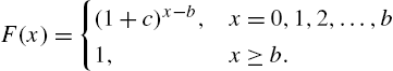
Example 2.15

In the continuous case, Block et al. (1998) have shown that for an absolutely continuous random variable X with interval, of support ![]() ,
, ![]() , if the reversed hazard rate is a constant
, if the reversed hazard rate is a constant ![]() for all
for all ![]() , then
, then ![]() ,
, ![]() and
and
and conversely. Thus, there does not exist an absolutely continuous distribution with constant reversed hazard rate on the positive real axis. We will now show that in the discrete case, reversed hazard rate can be constant when a subset of the set of nonnegative integers is as the support of X.
Example 2.16

The reversed hazard rate in this case is
and ![]() .
.
Remark 2.9
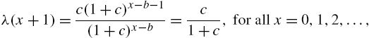
The terms in (2.56), for ![]() , are in geometric progression with a common ratio
, are in geometric progression with a common ratio ![]() and therefore, the successive terms are increasing, as opposed to the usual geometric distribution where the monotonicity is in the opposite direction. We will term (2.56) as the reversed geometric distribution with parameter c.
and therefore, the successive terms are increasing, as opposed to the usual geometric distribution where the monotonicity is in the opposite direction. We will term (2.56) as the reversed geometric distribution with parameter c.
This distribution has an important role in the sequel. Since it does not form part of the standard distributions discussed in the next chapter, some properties of the model (2.56) are presented here. First,

Thus, the distribution can be identified in practice for data for which the ratio of the successive frequencies, except the first, are nearly constant. The mean and variance are given by

and

For the geometric distribution, the hazard rate is constant which is equivalent to the lack of memory property. An analogous property in a reverse sense is satisfied by the reversed geometric law, as the next theorem shows.
Theorem 2.13
Proof
Eq. (2.58) can be restated as
Substituting (2.57) in (2.59), we readily have the ‘if’ part. Conversely, (2.59) is equivalent to the functional equation
where ![]() . To solve for
. To solve for ![]() , we set
, we set ![]() , so that
, so that
Iterating for t,
and so
Thus,

Summing for ![]() and using the fact that
and using the fact that ![]() , we get
, we get ![]() . Inserting the values of
. Inserting the values of ![]() in (2.60), we get
in (2.60), we get
Since ![]() , we should have
, we should have ![]() and setting
and setting ![]() , the distribution in (2.57) is recovered, as needed. □
, the distribution in (2.57) is recovered, as needed. □
Remark 2.10
The reversed lack of memory property implies that, given the lifetime of device is upto age x, the probability that the device fails at any age in ![]() is the same. Further, the distribution of such a lifetime is governed by the reversed geometric law.
is the same. Further, the distribution of such a lifetime is governed by the reversed geometric law.
Further discussions and application of these results can be seen in Nair and Sankaran (2013).
The definition in (2.53), when applied to the continuous case, has the form ![]() . This property is not shared in the discrete case. For reasons similar to those explained in Section 2.2 regarding the alternative hazard rate, a second definition for reversed hazard rate can be put forward as
. This property is not shared in the discrete case. For reasons similar to those explained in Section 2.2 regarding the alternative hazard rate, a second definition for reversed hazard rate can be put forward as
In this case,
or
Also,
and ![]() is determined from
is determined from
From the definitions in (2.61) and (2.53), the relationship between ![]() and
and ![]() is found to be
is found to be
It may be noticed that ![]() , is consistent with the value
, is consistent with the value ![]() .
.
2.7 Reversed Mean Residual Life
A second measure of interest in reversed time is the reversed mean residual life. Suppose a device has failed before attaining age t. Then, the random variable ![]() is the time elapsed since the device has failed, conditioned on the fact that its lifetime is less than t, and this is referred to as the reversed residual life or inactivity time of X. It is easy to see that
is the time elapsed since the device has failed, conditioned on the fact that its lifetime is less than t, and this is referred to as the reversed residual life or inactivity time of X. It is easy to see that ![]() has the distribution function
has the distribution function
The mean of this distribution is called the reversed mean residual life or mean inactivity time, and is denoted by ![]() . One can also define
. One can also define ![]() as
as
We define ![]() . Note also that
. Note also that ![]() . Goliforushani and Asadi (2008) have established the following properties of
. Goliforushani and Asadi (2008) have established the following properties of ![]() :
:
- (i)
 is an increasing function with
  ;
; - (ii)
 ;
; - (iii)
 cannot be a decreasing function for all x;
 - (iv)
- (v) If X has a finite support as
 , then

- and

- (vi) If
 is decreasing function of x, then is an increasing function of x;
 - (vii)

It is of interest to mention here that the notions of residual life and inactivity time have been extended to general coherent systems and their properties, mixture representations and stochastic orderings of various forms have been discussed by numerous authors; see, for example, Navarro et al. (2008, 2013), Zhang (2010), Goliforushani and Asadi (2011), Goliforushani et al. (2012), and Parvardeh and Balakrishnan (2013, 2014).
Example 2.19

In the case of geometric distribution, the hazard rate ![]() is constant and so is the mean residual life function
is constant and so is the mean residual life function ![]() , the two being related by
, the two being related by ![]() . We will show that a different scenario exists in the relationship between
. We will show that a different scenario exists in the relationship between ![]() and
and ![]() . For the reversed geometric law,
. For the reversed geometric law, ![]() , whereas
, whereas

which is a strictly increasing function of x. However, we can recover a distribution with constant reversed mean residual life by modifying the probability at ![]() .
.
Theorem 2.14
Proof
Remark 2.12
Remark 2.13
The reversed mean residual life can also be related to the alternative reversed hazard rate. From (2.62) and the identity in (iv) above, we have
In certain problems, it is more convenient to deal with the conditional mean
The corresponding results for ![]() is easily derived from those of
is easily derived from those of ![]() by using the above identity.
by using the above identity.
Relationship between ![]() and
and ![]() of a different nature, than those indicated above, that characterizes families of discrete distributions has been proposed in literature. The main results reviewed here are from Gupta et al. (2006) and Nair and Sudheesh (2008). We retain the same notation as in Section 2.3. Let
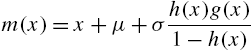
of a different nature, than those indicated above, that characterizes families of discrete distributions has been proposed in literature. The main results reviewed here are from Gupta et al. (2006) and Nair and Sudheesh (2008). We retain the same notation as in Section 2.3. Let ![]() be real-valued function such that
be real-valued function such that ![]() . Then, the probability mass function of X will be of the form
. Then, the probability mass function of X will be of the form
where ![]() and
and ![]() are the mean and standard deviation of
are the mean and standard deviation of ![]() satisfying
satisfying ![]() for some real-valued function
for some real-valued function ![]() if and only if
if and only if
with ![]() . The
. The ![]() function appearing in the above relationships is unique for a particular distribution and often assumes simple forms. Special cases of the form in (2.69) that includes various families like the discrete Pearson and Katz families and several individual distributions are discussed in Chapter 3. In practice, the formulas in (2.69) and (2.70) will work if we replace
function appearing in the above relationships is unique for a particular distribution and often assumes simple forms. Special cases of the form in (2.69) that includes various families like the discrete Pearson and Katz families and several individual distributions are discussed in Chapter 3. In practice, the formulas in (2.69) and (2.70) will work if we replace ![]() by function
by function ![]() , which can be determined from the data, without actually using
, which can be determined from the data, without actually using ![]() .
.
When any two of the functions ![]() ,
, ![]() and
and ![]() are known, the third can be determined from the identity
are known, the third can be determined from the identity
Similarly, we also have
and
From the last three forms, we arrive at
which will be useful in later chapters.
2.8 Reversed Variance Residual Life
Just as the mean of the reversed residual life ![]() , the variance of
, the variance of ![]() is also an important function reliability analysis, called the reversed variance residual life or variance inactivity time, and is denoted by
is also an important function reliability analysis, called the reversed variance residual life or variance inactivity time, and is denoted by ![]() . In algebraic manipulations, different expressions for
. In algebraic manipulations, different expressions for ![]() have been employed. These are
have been employed. These are
and
Further,

or
Example 2.20
Consider the geometric distribution ![]() in Example 2.2, for which
in Example 2.2, for which ![]() . Then, the conditional probability mass function of
. Then, the conditional probability mass function of ![]() is given by
is given by
We use (2.72) to calculate ![]() . For this, from (2.75), we have
. For this, from (2.75), we have
Differentiating with respect to q, we get

Simplifying so as to make the left hand side an expected value, we get

Differentiating (2.76) again with respect to q and rearranging the terms in the same manner, we get

The variance is now found from (2.72).
Various reliability functions in reversed residual lifetime for some distributions are exhibited in Table 2.4 and the graph of these functions for arithmetic distribution is presented in Fig. 2.3.
Table 2.4
The reversed hazard function, mean residual life and variance residual life for some distributions


In the continuous case, identities that connect the three functions ![]() ,
, ![]() and
and ![]() have been established. The corresponding results in the discrete case are
have been established. The corresponding results in the discrete case are
and
Eqs (2.78) and (2.79) are employed in finding ![]() when the others are known, especially in characterization problems and also in the discussions on the monotonicity of the reversed variance residual life function.
when the others are known, especially in characterization problems and also in the discussions on the monotonicity of the reversed variance residual life function.
As in the case of the usual mean and variance residual lives, we have

and
There are some special relationships between ![]() ,
, ![]() and
and ![]() that characterize certain families of distributions. Some important results in this connection are presented in the next two theorems.
that characterize certain families of distributions. Some important results in this connection are presented in the next two theorems.
Theorem 2.15

Proof

Theorem 2.16
The random variable X in Theorem 2.15 satisfies the property
a constant in ![]() , if and only if its distribution is (2.81) when
, if and only if its distribution is (2.81) when ![]() and the distribution is (2.68) when
and the distribution is (2.68) when ![]() .
.
Proof
First, we note that

or
Changing x to ![]() in (2.83) and then subtracting (2.83), we get
in (2.83) and then subtracting (2.83), we get
When (2.82) is satisfied with ![]() , from
, from
and (2.82), we obtain
Substituting in (2.84) and simplifying, we get
and hence ![]() is a constant and the distribution is (2.68). On the other hand, when the distribution is (2.68),
is a constant and the distribution is (2.68). On the other hand, when the distribution is (2.68), ![]() and then (2.74) yields
and then (2.74) yields
Also, ![]() , so that the theorem is proved when
, so that the theorem is proved when ![]() . In the more general case, when
. In the more general case, when ![]() , assume that X has distribution (2.81). Then,
, assume that X has distribution (2.81). Then,
Further, in formula (2.74), we have
Upon using the combinational identity

we have

Substituting for ![]() from (2.81) and simplifying (2.86), we get
from (2.81) and simplifying (2.86), we get
Now from (2.85),

and so the formula (2.74) yields

Thus,
Conversely, under the hypothesis of the theorem, we have
With the aid of (2.79), we write

The last equation leads to
which on solving using the boundary condition ![]() , gives
, gives
Setting ![]() so that
so that ![]() as stipulated, we have
as stipulated, we have
and hence the distribution is (2.81). □
Remark 2.14
Remark 2.15
Eq. (2.84) represents a family of finite range distributions that contains the uniform distribution for ![]() and the arithmetic law for
and the arithmetic law for ![]() .
.
Arising from characteristics of the finite range laws discussed above, we have some further characterizations. These results can be proved by invoking Cauchy-Schwarz inequality, as done in Theorems 2.6 and 2.7.
Theorem 2.17
Let X be a discrete random variable with the support ![]() . Then:
. Then:
- (i)
 with the equality holding if and only if X has reversed geometric law;
 - (ii)
 and the equality holds if and only if X follows distribution (2.68).
Theorem 2.18
Let X be a discrete random variable with the support ![]() . Then,
. Then,
if and only if the distribution of X is (2.81).
2.9 Odds Function
Along with the traditional reliability functions presented so far, there has been some interest in discovering the potential of odds function and log odds function in reliability analysis. The motivation for the consideration of these two functions are (i) they are easy to compute and interpret (ii) the estimation of these functions is relatively simpler, and (iii) the behaviour of other reliability functions can be ascertained through them.
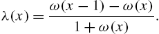
The concept of odds ratio originated from gambling wherein the odds of an event A against another event B is defined as the ratio ![]() . In reliability theory, we can take the event A as survival of age x and B as failure by age x. Then, the odds ratio of the events become a function of x. The odds ratio for surviving age x is defined as
. In reliability theory, we can take the event A as survival of age x and B as failure by age x. Then, the odds ratio of the events become a function of x. The odds ratio for surviving age x is defined as
and it is called the odds function for survival. Similarly, the odds function for failure by age x is
From the definitions, it follows that
- (i)
 ,
,  and
and  is decreasing,
 - (ii)
 ,
,  and
and  is increasing.
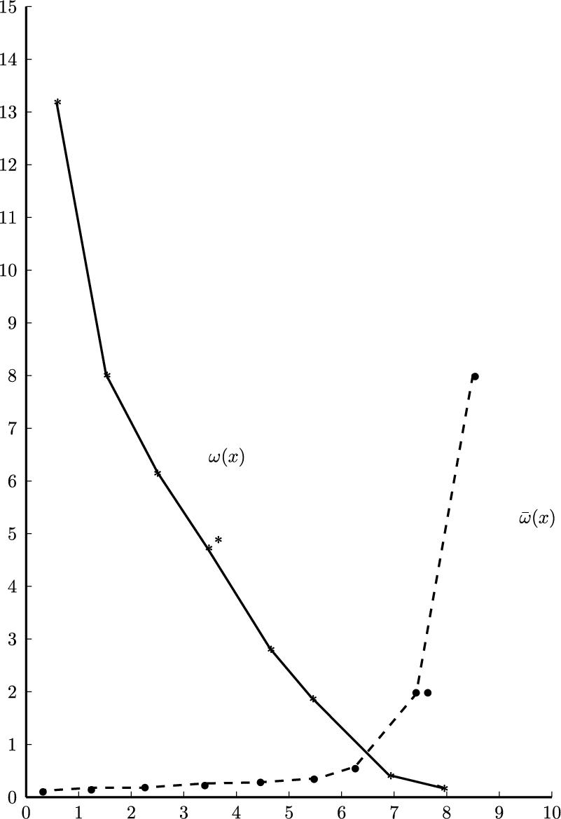
Odds functions ω and ![]() are important tools in survival analysis and medical studies in developing models for survival data and in comparing a treatment group with a control group. We refer to Collett (1994) and Kirmani and Gupta (2001) for further details. There has not been much study about the role of odds functions in reliability analysis, especially in the discrete case. We note that
are important tools in survival analysis and medical studies in developing models for survival data and in comparing a treatment group with a control group. We refer to Collett (1994) and Kirmani and Gupta (2001) for further details. There has not been much study about the role of odds functions in reliability analysis, especially in the discrete case. We note that
and

Accordingly, both ![]() and
and ![]() determine the distribution of X uniquely through the expressions
determine the distribution of X uniquely through the expressions
and
It is easy to see that the hazard and reversed hazard rates are
and
We can express the monotonicities of ![]() and
and ![]() in terms of
in terms of ![]() and
and ![]() .
.
Theorem 2.19
(i) ![]() is decreasing
is decreasing ![]() is decreasing
is decreasing ![]() is convex;
is convex;
(ii) ![]() is increasing
is increasing ![]() is increasing
is increasing ![]() is convex.
is convex.
Proof


Example 2.21
Consider the uniform distribution in Example 2.2. In this case,
The hazard and reversed hazard rates are obtained by using (2.91) and (2.92) as
Notice that ![]() is decreasing and
is decreasing and ![]() is increasing, so that the reverse implication
is increasing, so that the reverse implication ![]() increasing means
increasing means ![]() is increasing in (ii) is not true. However, it can be easily verified that
is increasing in (ii) is not true. However, it can be easily verified that ![]() is convex.
is convex.
The concepts based on residual life and reversed residual life can also be expressed in terms of odds functions. Recall that the survival function of the residual life ![]() is
is
The residual odds functions are then
or

and similarly
In terms of ![]() ,
,

and

Also, the mean residual life function is
Eq. (2.93) leads to the recurrence relation
Proof
By means of (2.91), we can write
In terms of the odds functions, the reversed mean residual life is

and so
□
In the same manner as we have proved Theorem 2.3, we note the following.
Instead of considering the odds functions, it is sometimes beneficial to use the odds rate defined as
The function ![]() is interpreted as the rate at which
is interpreted as the rate at which ![]() changes at age x. It has the following properties:
changes at age x. It has the following properties:
- (i)
 ;
; - (ii) The sequence of rates
 determine the distribution of X uniquely as
- (iii) If
 is decreasing (
 is concave), then
  is decreasing;
 - (iv) If is increasing, then is also increasing.
Example 2.22
Assume that ![]() ,
, ![]() . Writing
. Writing

Employing formula (2.96), we have
the survival function of the discrete uniform distribution.
Property (iii) of ![]() given above tells us that the class of distributions with decreasing
given above tells us that the class of distributions with decreasing ![]() is a subset of the decreasing failure rate class and also that a sufficient condition for failure rate to be decreasing is that
is a subset of the decreasing failure rate class and also that a sufficient condition for failure rate to be decreasing is that ![]() is concave. Thus, we have a stronger condition that assists in characterizing and modelling failure time data. Further, when
is concave. Thus, we have a stronger condition that assists in characterizing and modelling failure time data. Further, when ![]() is increasing,
is increasing, ![]() is also increasing, providing an alternative proof of (ii) in Theorem 2.3. For detailed discussion of the results in this section, we refer to Nair and Sankaran (2015b).
is also increasing, providing an alternative proof of (ii) in Theorem 2.3. For detailed discussion of the results in this section, we refer to Nair and Sankaran (2015b).
2.10 Log-odds Functions and Rates
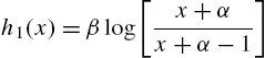
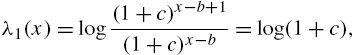
The log-odds functions and rates were introduced by Zimmer et al. (1998) as an alternative reliability measure and further propagated in the work of Wang et al. (2003, 2008). These functions were proposed as an alternative to the hazard rate in situations under which the device considered have high reliability or the corresponding hazard rate is non-monotone. When X is a discrete lifetime, Khorashadizadeh et al. (2013a) defined the log-odds function as
and the corresponding log-odds rate as
They have shown the following:
- (a)
 , where
  and
and  are the alternative reversed hazard and hazard rates of X discussed in Section 2.2;
 - (b)
 is characterized by
- where
 and
and  ;
; - (c) In terms of
 , we have
- and hence
- where
 ;
; - (d) X has increasing log-odds rate in terms of x (
 ) if and only if
  is convex with respect to x ().
From the above discussions, it is clear that ![]() is directly related to the alternative hazard and reversed hazard rates whereas
is directly related to the alternative hazard and reversed hazard rates whereas ![]() is related to the usual hazard rate. There are other mathematical properties that make
is related to the usual hazard rate. There are other mathematical properties that make ![]() and
and ![]() more desirable than their logarithms.
more desirable than their logarithms.
Theorem 2.22
Proof
By virtue of the properties of ![]() ,
,
is a survival function. Let ![]() denote the corresponding random variable. From the representation in (2.14), the cumulative hazard rate of
denote the corresponding random variable. From the representation in (2.14), the cumulative hazard rate of ![]() is
is
where ![]() is the alternative hazard rate of
is the alternative hazard rate of ![]() , and it satisfies
, and it satisfies
Now, from (2.100) and (2.101), we have
proving the first part. Using (2.99),
so that (2.98) holds. Since there is a one-to-one correspondence between ![]() and
and ![]() , they have the same support, and this completes the proof. □
, they have the same support, and this completes the proof. □
Some observations from Theorem 2.22 are as follows:
- (a) The converse of Theorem 2.22 is also true; that is, if
 is the survival function of a random variable
  satisfying (2.98), then
  is the survival function of a random variable X for which
  ;
; - (b) Since

- we have
- and

- (c) A parallel result that involves the odds function and the alternative reversed hazard rate
 is also possible. To see this, it is easy to recognize that
 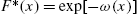 is a distribution function, with alternative reversed hazard rate
Since ![]() is a decreasing function,
is a decreasing function, ![]() is the rate at which
is the rate at which ![]() is decreasing and is therefore an odds rate. Thus, there exists a distribution specified by
is decreasing and is therefore an odds rate. Thus, there exists a distribution specified by ![]() for which the odds rate
for which the odds rate ![]() of
of ![]() is the reversed hazard rate of
is the reversed hazard rate of ![]() and the connection between the two is explained in the next theorem.
and the connection between the two is explained in the next theorem.
Theorem 2.23
Corresponding to a discrete random variable X with distribution function ![]() and odds rate
and odds rate ![]() , there exist another distribution function
, there exist another distribution function ![]() with the same support as
with the same support as ![]() and alternative reversed hazard rate
and alternative reversed hazard rate ![]() that satisfies
that satisfies
Also, ![]() and
and ![]() are related through
are related through
Conversely, if for two distribution functions ![]() and
and ![]() (2.103) holds, then
(2.103) holds, then ![]() .
.
Remark 2.16
Example 2.23

In this case,
and
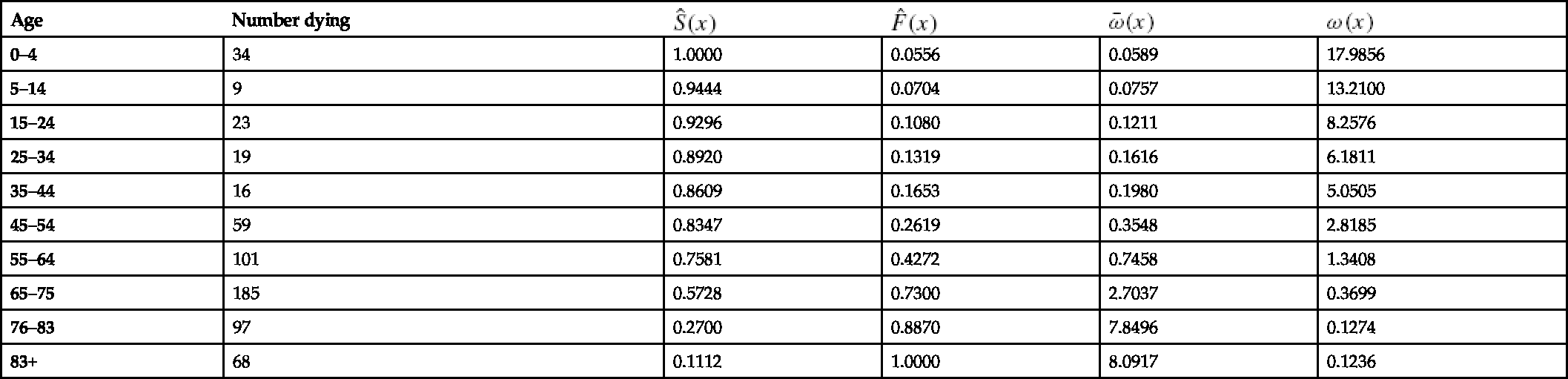
Example 2.24
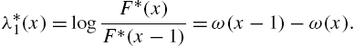
In this example, we present an analysis of real data on the number of deaths following surgery in a hospital in the US classified according to the age of the patients (Mosteller and Tukey, 1977). The survival function is estimated from the sample as
while
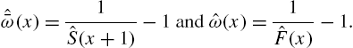
Table 2.5 presents the necessary calculations and Fig. 2.4 shows the shapes of the ![]() and
and ![]() curves.
curves.
Table 2.5
Estimation of ω(x) and ![]()
| Age | Number dying |
|
|
|
|
|---|---|---|---|---|---|
| 0–4 | 34 | 1.0000 | 0.0556 | 0.0589 | 17.9856 |
| 5–14 | 9 | 0.9444 | 0.0704 | 0.0757 | 13.2100 |
| 15–24 | 23 | 0.9296 | 0.1080 | 0.1211 | 8.2576 |
| 25–34 | 19 | 0.8920 | 0.1319 | 0.1616 | 6.1811 |
| 35–44 | 16 | 0.8609 | 0.1653 | 0.1980 | 5.0505 |
| 45–54 | 59 | 0.8347 | 0.2619 | 0.3548 | 2.8185 |
| 55–64 | 101 | 0.7581 | 0.4272 | 0.7458 | 1.3408 |
| 65–75 | 185 | 0.5728 | 0.7300 | 2.7037 | 0.3699 |
| 76–83 | 97 | 0.2700 | 0.8870 | 7.8496 | 0.1274 |
| 83+ | 68 | 0.1112 | 1.0000 | 8.0917 | 0.1236 |
 .
.2.11 Mixture Distributions
The role of mixture distributions in reliability studies was mentioned earlier in Section 2.1. When the mixture is of the form (1.11), we have
and
where ![]() is the probability mass function and
is the probability mass function and ![]() (
(![]() ) is the survival function corresponding to
) is the survival function corresponding to ![]() (
(![]() ). If
). If ![]() ,
, ![]() and
and ![]() , respectively, denote the hazard rates of f,
, respectively, denote the hazard rates of f, ![]() and
and ![]() , it is easy to see that
, it is easy to see that
where

Likewise, for the reversed hazard rates λ, ![]() and
and ![]() of
of ![]() and
and ![]() , respectively, we have
, respectively, we have
with
Finite mixtures of two components are commonly used in heterogeneous populations in which the elements are classified into two categories. It follows from (2.105) that
and also that
whenever ![]() for all x.
for all x.
Theorem 2.24
If ![]() for all x,
for all x, ![]() is an increasing function.
is an increasing function.
Proof
We have
The sign of the previous equation depends on

since ![]() . Thus,
. Thus, ![]() is increasing. This result has the interpretation that when the lifetime distribution is a mixture, the weakest items will die out first.
is increasing. This result has the interpretation that when the lifetime distribution is a mixture, the weakest items will die out first.
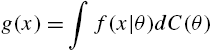
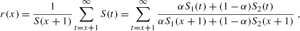
When the distribution of X is indexed by a parameter θ, where θ is the value of a random variable Θ defined on ![]() with distribution function
with distribution function ![]() , from (1.3), the survival function and the probability mass function of X are given by
, from (1.3), the survival function and the probability mass function of X are given by
and
so that the mixture has its hazard rate as

where
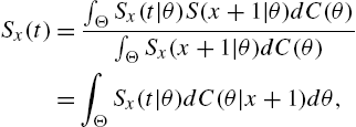
is the conditional hazard rate of X, given ![]() , and
, and
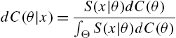
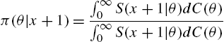
is the conditional density function of θ, given ![]() . When
. When ![]() , the density function of Θ,
, the density function of Θ, ![]() , defines the conditional probability density function of θ with the same support as that of Θ. In a Bayesian context,
, defines the conditional probability density function of θ with the same support as that of Θ. In a Bayesian context, ![]() can be viewed as a prior distribution of θ, and
can be viewed as a prior distribution of θ, and ![]() as the posterior distribution of θ after observing the data on X. Models in which θ is regarded as random are called frailty models which are extensively discussed in survival analysis. In particular, if a representation of the form
as the posterior distribution of θ after observing the data on X. Models in which θ is regarded as random are called frailty models which are extensively discussed in survival analysis. In particular, if a representation of the form
holds, then from (2.17), we have the alternative hazard rates of ![]() , say
, say ![]() , and S satisfy the relationship
, and S satisfy the relationship
We say that a random variable ![]() with survival function
with survival function ![]() is the proportional hazard rates model corresponding to X with survival function
is the proportional hazard rates model corresponding to X with survival function ![]() . □
. □
Some similar results exist for reversed hazard rates as well.
Theorem 2.25
In the case of reversed rate functions, if ![]() for all x, then
for all x, then ![]() is an increasing function.
is an increasing function.
Proof
We have
The sign of the left hand side depends on

which is non-negative since ![]() for all x. Hence,
for all x. Hence, ![]() is an increasing function.
is an increasing function.
Assuming θ to be random with distribution function ![]() , the mixture has reversed hazard rate
, the mixture has reversed hazard rate

where
is the conditional reversed hazard rate of X, given ![]() , and
, and
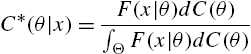
is the conditional distribution function of θ, given ![]() . As before, if a representation of the form
. As before, if a representation of the form
holds, then the reversed hazard rates λ of ![]() and F satisfy the relationship
and F satisfy the relationship
In this case, we say that ![]() is the reversed proportional hazard rates model of F. □
is the reversed proportional hazard rates model of F. □
Nelson (1982) has mentioned that units manufactured in different production periods may have different life distributions due to difference in design, raw materials, handling, etc., and it may therefore be necessary to identify production period, customer environment, etc. that result in poor units, for remedial action on that part of the population. Cox (1959) analyzed data on failure times using mixture models by classifying the cause of failure as identified or not; see also Mendenhall and Hader (1958) and Cheng et al. (1985). Identification of the life distribution is crucial in such cases. One way in which such identification is possible is to use characterization theorems that involve various reliability functions or relationships between them. Nair et al. (1999) proposed certain relationships between the hazard rate and the mean residual life that characterize some mixture distributions for the purpose.
Theorem 2.26


Corollary 2.27


In Theorem 2.26, we have used the mean residual life of the mixture of the form in (2.104). According to Definition 2.20, it is calculated as
where ![]() and
and ![]() are the survival functions of the component distributions. Eq. (2.108) is expressible as
are the survival functions of the component distributions. Eq. (2.108) is expressible as
with
and ![]() and
and ![]() are the mean residual life functions of the component distributions. When
are the mean residual life functions of the component distributions. When ![]() is indexed by the values of a non-negative continuous random variable Θ, the residual life distribution becomes
is indexed by the values of a non-negative continuous random variable Θ, the residual life distribution becomes

as a naturally corollary of the basic definition in (2.19). Eq. (2.109) is equivalent to
where
is the distribution function of Θ given ![]() .
.
Apart from the hazard function and mean residual life function, higher moments of residual life can also be used for characterizing life distributions. Two such results are established in Nair et al. (1999).
Theorem 2.28
If ![]() , the identity
, the identity
- (a)
- holds if and only if X is distributed as geometric mixture in (2.107);
- (b)
- where
- and
- if and only if X has a three-component geometric mixture

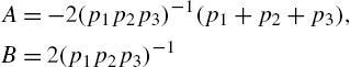
These authors have pointed out with the help of simulated data that Theorem 2.26 is useful in model identification and inference. If the plots of the estimates ![]() fall along a straight line, the distribution is mixture of geometric. A quick estimate of the parameters
fall along a straight line, the distribution is mixture of geometric. A quick estimate of the parameters ![]() and
and ![]() is obtained from the slope and intercept of the fitted line, or more accurately from a least-square fit of the line. One can estimate α by equating the sample mean with
is obtained from the slope and intercept of the fitted line, or more accurately from a least-square fit of the line. One can estimate α by equating the sample mean with
after substituting the estimate of ![]() and
and ![]() . Nair (1983b) addressed the estimation problem by matching the factorial moments of the sample with those of the population. Denoting by
. Nair (1983b) addressed the estimation problem by matching the factorial moments of the sample with those of the population. Denoting by ![]() ,
, ![]() and
and ![]() the first three sample factorial moments, the equations to be solved are as follows:
the first three sample factorial moments, the equations to be solved are as follows:
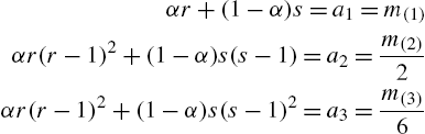
with ![]() and
and ![]() . After some algebra, the quadratic equation
. After some algebra, the quadratic equation
is obtained, which can be solved for s. Now r and α are calculated from
If there are two admissible solutions for s in the above quadratic equation, the one that gives better fit is chosen as the final estimate.
Sometimes, mixtures of a more general form

or

where ![]() are real numbers, not necessarily all positive, satisfying
are real numbers, not necessarily all positive, satisfying ![]() are also considered. They are of practical significance representing distributions of order statistics, coherent systems and inference in step-stress models. Discussions of these aspects in the continuous case can be seen in Navarro and Rychlik (2007), Navarro and Shaked (2006), Balakrishnan et al. (2007, 2009), Balakrishnan and Cramer (2008), and Balakrishnan and Xie (2007). When some of the mixing constants are negative, such mixtures are called generalized mixtures. The representation in (2.110) can be expressed as (Navarro and Hernandez, 2004) as
are also considered. They are of practical significance representing distributions of order statistics, coherent systems and inference in step-stress models. Discussions of these aspects in the continuous case can be seen in Navarro and Rychlik (2007), Navarro and Shaked (2006), Balakrishnan et al. (2007, 2009), Balakrishnan and Cramer (2008), and Balakrishnan and Xie (2007). When some of the mixing constants are negative, such mixtures are called generalized mixtures. The representation in (2.110) can be expressed as (Navarro and Hernandez, 2004) as
with ![]() ,
,

Then,
and the relationship for ![]() becomes
becomes
where ![]() is the mean residual life function of
is the mean residual life function of ![]() .
.
Recalling the formula for the reversed mean residual life of X as

we see that for the two-component mixture we have
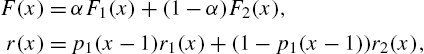
where ![]() and
and ![]() are the reversed mean residual lives of
are the reversed mean residual lives of ![]() and
and ![]() and
and ![]() is as defined in (2.106). Eliminating
is as defined in (2.106). Eliminating ![]() from
from
and (2.106), a relationship connecting the reversed mean residual life ![]() and the reversed hazard rate
and the reversed hazard rate ![]() of the mixture can be expressed in the form
of the mixture can be expressed in the form
where


Example 2.25
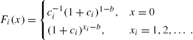
The relationship given above provides a plot of ![]() as a decreasing straight line which is easy to verify. Notice that (2.115) is a characteristic property of this distribution.
as a decreasing straight line which is easy to verify. Notice that (2.115) is a characteristic property of this distribution.
2.12 Weighted Distributions
Recalling the definition of the weighted distribution in (1.20) that
and the expression of the survival function in (1.21) given by
the mean residual lives of X and ![]() satisfy the relationship
satisfy the relationship

As special cases, we have

Denoting ![]() and
and ![]() , for the hazard rate and the mean residual life of the equilibrium random variable
, for the hazard rate and the mean residual life of the equilibrium random variable ![]() (Section 1.4), we have from Nair et al. (2012b) that
(Section 1.4), we have from Nair et al. (2012b) that
and
In particular, for the first-order equilibrium random variable ![]() (Nair and Hitha, 1989), we have
(Nair and Hitha, 1989), we have

so that the hazard rate of ![]() is the reciprocal of the mean residual life of
is the reciprocal of the mean residual life of ![]() . Furthermore, we have
. Furthermore, we have

From the above identities, Nair and Hitha (1989) have also shown the following:
(a) a mean residual life of the form ![]() characterizes the geometric, Waring and negative hyper-geometric distributions according as
characterizes the geometric, Waring and negative hyper-geometric distributions according as ![]() ,
, ![]() and
and ![]() , respectively;
, respectively;
(b) the random variables X and ![]() are such that
are such that ![]() (
(![]() ) if and only if X is geometric for
) if and only if X is geometric for ![]() (
(![]() ), Waring for
), Waring for ![]() (
(![]() ) and negative hyper-geometric for
) and negative hyper-geometric for ![]() (
(![]() ).
).
More general characterizations covering the original and the nth-order equilibrium distributions have been provided by Nair et al. (2012b) as follows:
- (a)
 for all x and
  ;
; - (b)
 , for all x and ;
 - (c) the variance residual life of
 ,
,
holds if and only if X has one of the above three distributions, the geometric (![]() ,
, ![]() ,
, ![]() ), Waring (
), Waring (![]() ,
, ![]() ,
, ![]() ), and negative hyper-geometric (
), and negative hyper-geometric (![]() ,
, ![]() ,
, ![]() ).
).
In particular, ![]() characterizes the geometric distribution. So also the property
characterizes the geometric distribution. So also the property
a constant, for all x and ![]() .
.
Li (2011) obtained formulas for the equilibrium distribution of the n-fold convolution of ![]() and mixtures. If
and mixtures. If ![]() is the n-fold convolution of f (see Section 1.5) and
is the n-fold convolution of f (see Section 1.5) and ![]() is the m-th order equilibrium distribution of
is the m-th order equilibrium distribution of ![]() , then
, then

where ![]() is the rth factorial moment of
is the rth factorial moment of ![]() ,
, ![]() ,
, ![]() .
.
When the baseline distribution of X is ![]() , where θ is the realization of a continuous random variable Θ, the mixture (Section 1.3)
, where θ is the realization of a continuous random variable Θ, the mixture (Section 1.3)
has nth order equilibrium distribution
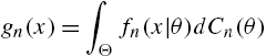
where
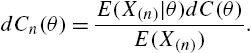
Example 2.26
It has been shown in Example 1.2 that the nth order equilibrium distribution of a geometric variable X is the same as the distribution of X. Now, in this case, we have
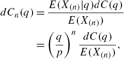
showing that ![]() is also a mixture geometric law.
is also a mixture geometric law.
Finally, we look at the relationships between various reliability measures in reversed time in the original and weighted versions. For this purpose, we note that the distribution function of the weighted law is given by
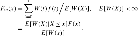
Accordingly, the reversed failure rate of ![]() becomes
becomes
Similarly, from (2.64),
gives

These identities, relationships and formulas are helpful while discussing properties of ageing concepts of weighted distributions and their relationships with those of the baseline distribution.