
Solution Execution and Result
Abstract
In this chapter, we will go through to implementing IDSAODV as a solution versus this attack and will see its effects on AODV performance faces with single and multiple black hole attack. When we examine the trace file of the simulations that include one black hole node, we observe that after a while, second RREP message comes to source node from the real intermediate node.
Keywords
Black hole attack; AODV routing protocol; IDSAODV; AODV performance faces
5.1 Introduction
In previous chapter, it has implemented the black hole attack on AODV routing protocol and observed the effects of single and multiple attack on this protocol. In this chapter, we will go through to implementing IDSAODV as a solution versus this attack and will see its effects on AODV performance faces with single and multiple black hole attack.
5.2 An Outline of Investigation
In previous chapter, it explained how black hole attack is implemented in NS2 and which results are obtained from the simulations. When we examine the trace file of the simulations that include one black hole node, we observe that after a while, second RREP message comes to source node from the real intermediate node.
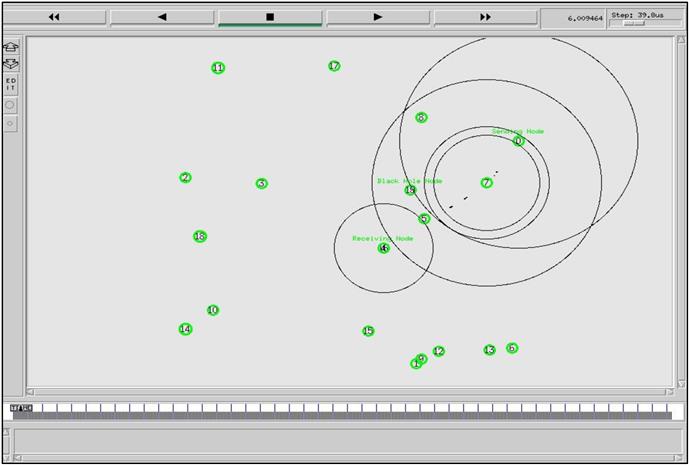
To figure out how the second packet came to source node, it has created a simulation scenario with node positions as shown in Fig. 5.1. In the scenario, node 0 is the sending node, node 1 is black hole node, and node 4 is the receiving node. As the black hole send an RREP message without checking the tables, we assume that it is more likely for the first RREP to arrive from the black hole. In some cases, this idea may not work. For instance; the second RREP can be received at source node from an intermediate node which has fresh enough information about the destination node or the second RREP message may also come from the black hole node if the real destination node is nearer than the black hole node or in networks with multiple black hole nodes, second RREP can receive from other black hole nodes. These examples are extendable according to node condition in the network topology. In this book, it is tried to find out how IDSAODV eliminates the black hole effects in AODV with single black hole node and AODV with multiple black hole nodes, and if it improves the network performance or not.
5.3 Execution of the Solution in NS-2
To evaluate effects of the proposed solution, first, it needs to be implemented in NS-2. Therefore, should simulate the “AODV” protocol, changing it to “IDSAODV” as it did “blackholeAODV” before. To implement, the black hole has been changed the receive RREP function (recvRequest) of the blackholeaodv.cc file but to implement the solution had to change the receive RREP function (recvReply) and create RREP caching mechanism to count the second RREP message.
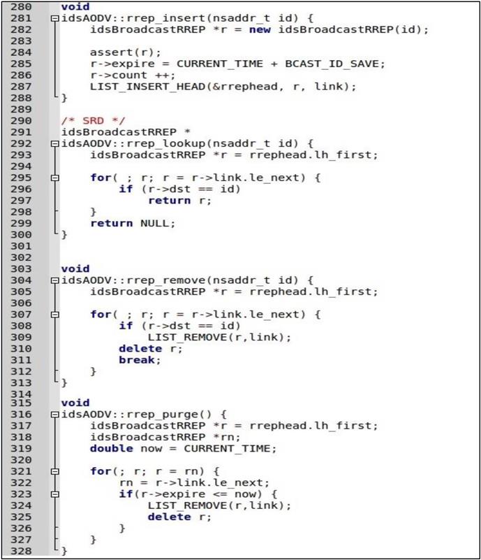
Fig. 5.1 shows the RREP caching mechanism. The “rrep_insert” function is for adding RREP messages, “rrep_lookup” function is for looking any RREP message up if it exists, “rrep_remove” function is for removing any record for RREP message that arrived from defined node and “rrep_purge” function is to delete periodically from the list if it has expired. It has chosen this expire time “BCAST_ID_SAVE” as 6 (mean seconds).
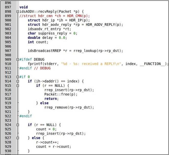
In the “recvReply” function, first we control if the RREP message arrived for itself and if it did, function looks the RREP message up if it has already arrived. If it did not, it inserts the RREP message for its destination address and returns from the function. If the RREP message is cached before for the same destination address, normal RREP function is carried out. Afterwards, if the RREP message is not meant for itself the node forwards the message to its appropriate neighbor. Fig. 5.2 shows how the receive RREP message function of the IDSAODV is carried out.
5.4 Testing the IDSAODV
For implementing the IDSAODV protocol in NS-2, we tried it in a Tcl simulation. In the scenario of the simulation, there are seven motionless nodes and node positions are the same as in the test simulation of the two RREP messages. In this simulation, IDSAODV protocol is used instead of AODV for all nodes except the black hole node (Node 1). To change the AODV protocol to IDSAODV, we only change “$ns node-config-adhocRouting idsAODV”. When the simulation is compiled, we saw that sending node is sending the messages to receiving node properly. Fig. 5.3 shows that CBR packets are reaching the destination node as expected.
In the test simulation, it should be ensured that the IDSAODV implementation is correctly working. Then, the same simulations will be performed on the scenarios which have been used in Chapter 4 to compare the performance of IDS approach.
5.5 Simulation of IDSAODV and Appraisal of Results
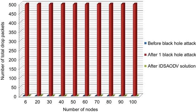
To be able to evaluate if the proposed solution has been successful, we used same scenarios and simulation parameters as described in Chapter 4 and also to be able to obtain the simulation results, it has been used a similar batch file adapted for idsaodv. Tables 5.1–5.8 compare effects of IDSAODV network with single and multiple black hole networks. Total drop packet for single black hole as we can see in Table 5.1 is almost zero.
Table 5.1
| Number of nodes | 6 | 20 | 30 | 40 | 50 | 60 | 70 | 80 | 90 | 100 |
| Before black hole attack | 0 | 0 | 0 | 0 | 0 | 0 | 0 | 0 | 0 | 0 |
| After one black hole attack | 498 | 498 | 498 | 498 | 498 | 498 | 498 | 498 | 498 | 498 |
| After IDSAODV solution | 1 | 1 | 0 | 0 | 0 | 0 | 0 | 0 | 0 | 0 |
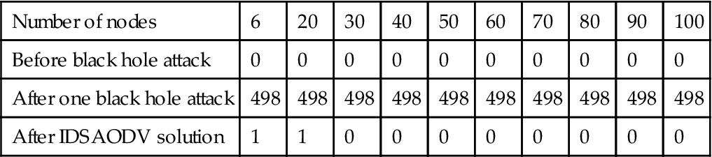
Table 5.2
| Number of nodes | 6 | 20 | 30 | 40 | 50 | 60 | 70 | 80 | 90 | 100 |
| Before black hole attack | 0 | 0 | 0 | 0 | 0 | 0 | 0 | 0 | 0 | 0 |
| After two black hole attack | 498 | 498 | 498 | 498 | 498 | 498 | 498 | 498 | 498 | 498 |
| After IDSAODV solution | 0 | 1 | 1 | 1 | 1 | 1 | 1 | 1 | 1 | 1 |
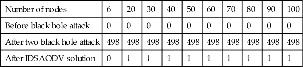
Table 5.3
| Number of nodes | 6 | 20 | 30 | 40 | 50 | 60 | 70 | 80 | 90 | 100 |
| Before black hole attack | 0.116364 | 0.11639 | 0.1059 | 0.101903 | 0.100342 | 0.100103 | 0.078637 | 0.078323 | 0.065856 | 0.0551 |
| After one black hole attack | 0 | 0.06141 | 0.0596 | 0 | 0 | 0 | 0.024322 | 0.01776 | 0.017762 | |
| After IDSAODV solution | 0.216364 | 0.21639 | 0.2059 | 0.201903 | 0.200342 | 0.200103 | 0.178637 | 0.178323 | 0.165856 | 0.1551 |
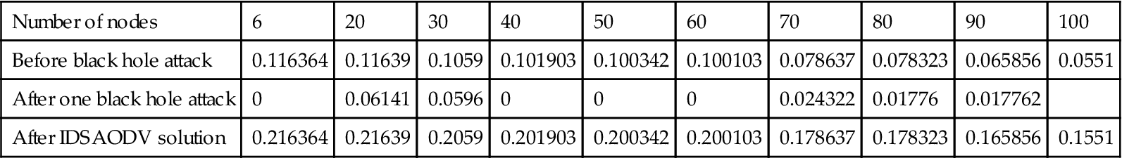
Table 5.4
| Number of nodes | 6 | 20 | 30 | 40 | 50 | 60 | 70 | 80 | 90 | 100 |
| Before black hole attack | 0.116364 | 0.116387 | 0.1059 | 0.101903 | 0.100342 | 0.100103 | 0.078637 | 0.078323 | 0.065856 | 0.0551 |
| After two black hole attack | 0 | 0.023582 | 0.02392 | 0 | 0 | 0 | 0 | 0.17523 | 0.017482 | 0.018422 |
| After IDSAODV solution | 0.226364 | 0.226387 | 0.2159 | 0.211903 | 0.210342 | 0.210103 | 0.188637 | 0.188323 | 0.175856 | 0.1651 |
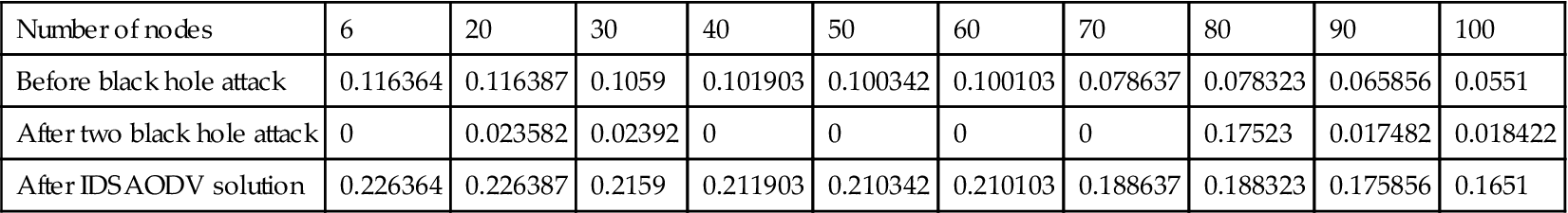
Table 5.5
| Number of nodes | 6 | 20 | 30 | 40 | 50 | 60 | 70 | 80 | 90 | 100 |
| Before black hole attack | 0.002 | 0.005 | 0.0079 | 0.01 | 0.015 | 0.014 | 0.016 | 0.024 | 0.026 | 0.029 |
| After two black hole attack | 0.001 | 0.01 | 0.009 | 0.016 | 0.017 | 0.018 | 0.02 | 0.026 | 0.028 | 0.03 |
| After IDSAODV solution | 0.003 | 0.007 | 0.008 | 0.012 | 0.015 | 0.016 | 0.019 | 0.024 | 0.026 | 0.029 |

Table 5.6
| Number of nodes | 6 | 20 | 30 | 40 | 50 | 60 | 70 | 80 | 90 | 100 |
| Before black hole attack | 0.002 | 0.005 | 0.0089 | 0.01 | 0.015 | 0.014 | 0.016 | 0.024 | 0.026 | 0.029 |
| After two black hole attack | 0.004 | 0.01 | 0.012 | 0.016 | 0.017 | 0.018 | 0.021 | 0.025 | 0.027 | 0.03 |
| After IDSAODV solution | 0.003 | 0.007 | 0.01 | 0.01 | 0.016 | 0.016 | 0.018 | 0.024 | 0.026 | 0.029 |
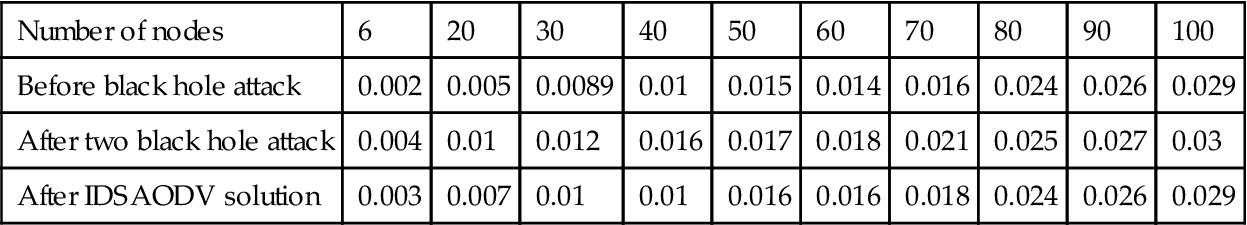
Table 5.7
Packet Delivery Ratio Comparison
| Number of nodes | 6 | 20 | 30 | 40 | 50 | 60 | 70 | 80 | 90 | 100 |
| Before black hole attack | 1 | 1 | 1 | 1 | 1 | 1 | 1 | 1 | 1 | 1 |
| After two black hole attack | 0 | 0 | 0 | 0 | 0 | 0 | 0 | 0 | 0 | 0 |
| After IDSAODV solution | 1 | 0.998 | 1 | 1 | 1 | 1 | 1 | 1 | 1 | 1 |
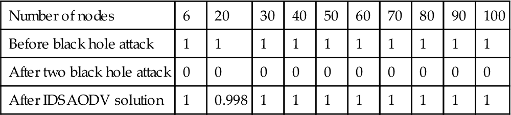
Table 5.8
Packet Delivery Ratio Comparison
| Number of nodes | 6 | 20 | 30 | 40 | 50 | 60 | 70 | 80 | 90 | 100 |
| Before black hole attack | 1 | 1 | 1 | 1 | 1 | 1 | 1 | 1 | 1 | 1 |
| After two black hole attack | 0 | 0 | 0 | 0 | 0 | 0 | 0 | 0 | 0 | 0 |
| After IDSAODV solution | 1 | 0.998 | 0.998 | 0.998 | 0.998 | 0.998 | 0.998 | 0.998 | 0.998 | 0.998 |
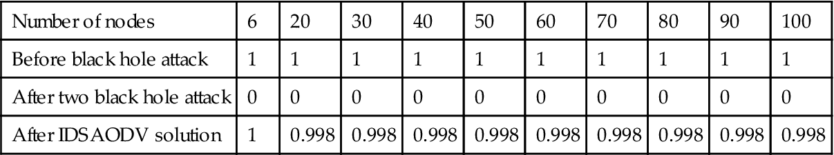
Fig. 5.4 is drawn from above table’s data which can compare total drop packets before black hole attack, after one black hole attack and after using IDSAODV solution:
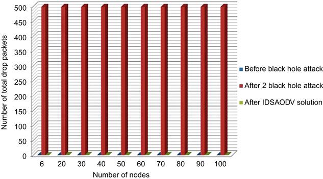
As shown in Table 5.2, total drop packet for multiple black hole attacks after using IDSAODV is almost zero too.
Fig. 5.5 is drawn from above table’s data which can compare total drop packets before black hole attack, after two black hole attacks and after using IDSAODV solution:
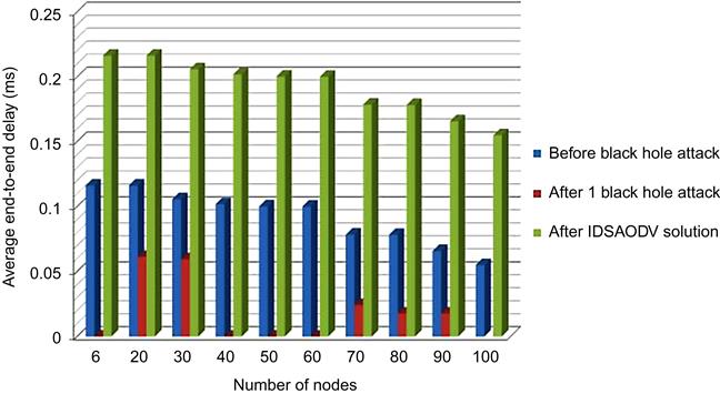
But average end-to-end delay (as shown in Table 5.3) after using IDSAODV increase and it is because of skipping first route reply.
Fig. 5.6 is drawn from above table’s data which can compare end-to-end delay before black hole attack, after one black hole attack and after using IDSAODV solution:
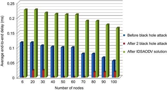
Same problem we have for end-to-end delay with IDSAODV for multiple black hole attacks, Table 5.4 shows the data came out from simulation:
Fig. 5.7 is drawn from above table’s data which can compare end-to-end delay before black hole attack, after two black hole attacks and after using IDSAODV solution.
Routing request overhead after using IDSAODV decrease a little bit compared with black hole AODV but it is higher than AODV before black hole attack and it is because of increasing routing request compared with AODV because of skipping first route reply. We can observe the data came out from routing overhead simulation in Table 5.5.
Fig. 5.8 is drawn from above table’s data which can compare routing overhead before black hole attack, after one black hole attack and after using IDSAODV solution:
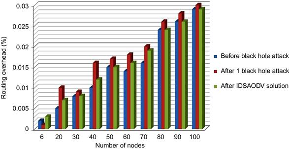
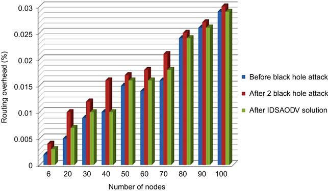
Table 5.6 shows the result of routing overhead simulation after using IDSAODV solution for multiple black hole attacks:
Fig. 5.9 is drawn from above table’s data which can compare routing overhead before black hole attack, after two black hole attacks and after using IDSAODV solution:
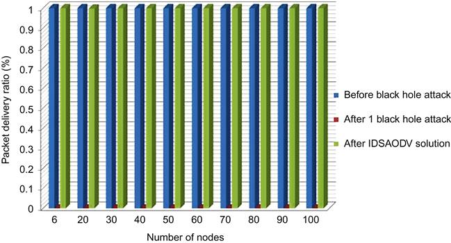
In Table 5.7, you can see which packet delivery ratio after IDSAODV is equaled one, and it means almost all of the packets that have been sent by sender, received by destination node:
Fig. 5.10 is drawn from above table’s data which can compare packet delivery ratio before black hole attack, after one black hole attack and after using IDSAODV solution:
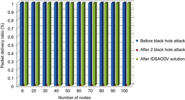
Packet delivery ratio for multiple black hole attacks also after using IDSAODV improved to almost one, we can see the result of simulation in Table 5.8:
Fig. 5.11 is drawn from above table’s data which can compare packet delivery ratio before black hole attack, after two black hole attacks and after using IDSAODV solution:
5.6 Summary
In this chapter, we simulated IDSAODV solution for observing its effects on multiple black hole AODV performance, after that compared the results of this simulation with multiple black hole AODV. According the results of this chapter, IDSAODV can improve performance of black hole AODV.