Chapter 1. The Tao of Dynamic Workflow
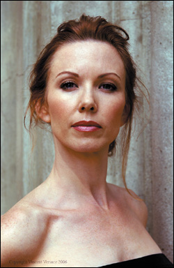
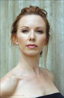
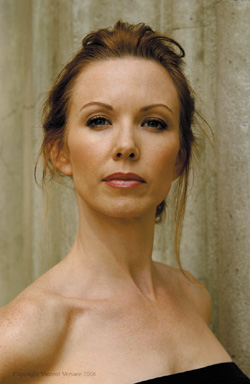
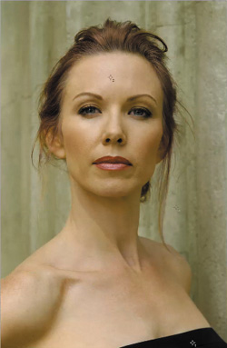
Figure 1.0.1. Before
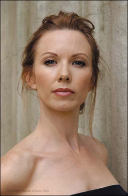
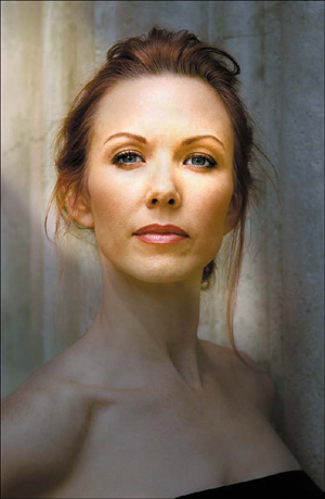
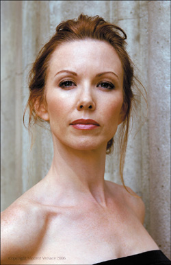
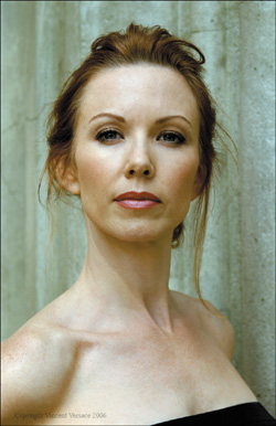
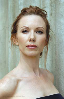
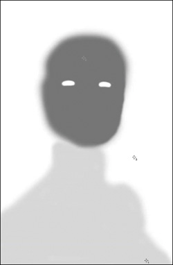
Figure 1.0.2. After
Practice doesn’t make perfect. Perfect practice makes perfect. You first have to practice at practicing.
—Vince Lombardi
This chapter deals with how to analyze an image and develop a dynamic, image-specific workflow, so that you can achieve in the print, the image as you conceptualized it. I place special focus on image mapping and how to do basic lighting in Photoshop. I also take a broader look at how to approach images and think about them. This lesson is about learning how to practice at practicing and then about how to find the path to perfect practice.
Revisiting Shibumi: The Art of Perfect Practice
My wish for this book was to make each chapter reflect, as closely as possible, an actual workflow—not some idealized sequence. Because workflow is fluid, and books are static, Acme Educational allowed me to use their high resolution computer screen grabs (frames from their 1200×1600 QuickTime movie) as part of each lesson in this book. But because some of you learn better by reading, some by seeing, and some do best using both, if you wish, you can purchase all the lessons from this book as a video set at www.acmeeducational.com. Both this book and the Acme tutorial are designed to stand alone, but they are mutually supportive.
Of all the lessons in this book, “Shibumi: The Art of Perfect Practice,” is the one to which I return again and again. When I originally created the image that I have used in this lesson, I learned a lot of the things that eventually led to the creation of my first book, Welcome to Oz. But, perhaps the most important thing that I learned is that impossible is just an opinion.
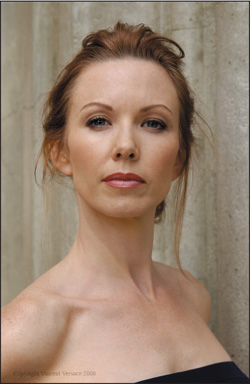
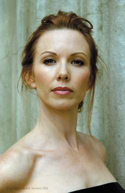
The image in this chapter is a picture of the actress Challen Cates from a photo shoot that I did in Los Angeles using a single piece of lighting gear, a 6′×3′ diffuser. Why a single piece of lighting gear? Simple—the lighting equipment I planned to use did not show up when I did. I had planned to use hot lights and reflectors, but when the lights did not show up, I was three hours away from my studio with only the diffuser that I had loaded, as an afterthought, into my assistant’s car. My choices were either to react to the situation and call it a day, or be proactive and go ahead with the shoot believing that by adapting and improvising, I would be able to achieve my original vision. Choosing to be proactive, I had my assistant hold the diffuser over Challen’s head so that she was evenly lit. Doing this would give me the best possible source file with which to work so that I could later light her properly in the computer. The techniques that I had to develop in order for me to achieve my original vision are the techniques that I want to share with you.
Note
Every image in this book marks a significant milestone in the development of my approach to creating images. Each represents a moment of discovery in which I found a new way to create, in print, what my eye had initially determined should be there.
I believe that it is best to approach Photoshop preemptively, to get it right in the camera, and that Photoshop is best used as an emery board and not a jackhammer. Even when the situation does not lend itself to getting it perfect, as in the case of the Challen Cates shoot, at the time of capture you should get as much right as possible.
In order to know how to get it right in the camera, which is the beginning of the process, you must understand the middle and end of the process as well. The middle of the process is the manipulation of the file in Photoshop and its end is the print, which is your voice, your vision.
This lesson will teach you how to analyze an image and optimize it. Image optimization is a process of refinement. First you make broad strokes that you later refine (what I call working from the global to the granular), removing everything that is not your vision, so all that remains is the image that you envisioned. You will also learn how to develop a dynamic, image-specific workflow so that you can achieve in the print the image as you conceptualized it. You will be able to do this because you will gain an understanding of how to maximize capture, so that manipulation of the file in Photoshop will result in the print that you wanted to achieve. Because of the circumstances of the Challen Cates shoot, the image that I had in my head when I captured it was nothing like the image I was forced to take—an image with almost no variation in light, dark, contrast, saturation, focus, or blur. I knew, however, that if I kept my initial vision in my head, using Photoshop, I could create those variations within that picture, so that it would be transformed into what I knew it should become.
IMPORTANT: Before You Begin This Lesson
If you have not downloaded the free plug-ins, the demo plug-ins, and source files from the download site for this lesson, as well as all the other files that are provided for the lessons in this book, go to: http://www.welcome2oz.com. All of the URLs that you need are located there, and you should do this before you go any further.
Note
All of the lessons have instructions on how to do them without the demo software, but when it comes to the free plug-ins (except in one instance), there is no alternative approach available in Photoshop. The reason for this is either that there is no way in Photoshop to accomplish what the plug-ins do, or that the plug-in does a better job. Also, the plug-ins are free with this book. One-hundred percent of my images see at least two of the plug-ins you now own. I highly recommend that you try them.
Each source file has two versions for all of the lessons in this book: one that contains all of the image maps that I created, and one that has only the source files. I urge you to use your own image maps, but they are best used if you have a tablet or pen-based display like I do. (I prefer a Wacom Cintiq or an Intuos 4 tablet.) If you have neither, or simply want to get right to the lesson, then use the source files with the image maps that I have provided.
The Secret of Dynamic Workflow
Workflow is a flexible series of steps that one follows to efficiently and accurately realize your vision.
—R. Mac Holbert
No two images are the same, so no two images will ever require the identical workflow, therefore, a standard workflow recipe does not exist. Some images are simply easier to work with than others, but before you begin, you may not know how much difficulty you will encounter. Your workflow must be flexible enough to accommodate any level of complexity.
Workflow is the operational aspect of a work procedure (in this case, producing a final image) and includes: how tasks are structured, their relative order, and how they are synchronized. A dynamic workflow is one in which you allow yourself mental flexibility when you work on an image. It is about figuring out how to process your file in order to create that which you hold in your mind’s eye. By approaching workflow dynamically, you not only gain total artistic control, even your file structure will be flexible, so that as technology and your skills improve, you can return to your files and re-interpret them.
A dynamic workflow is about making things as simple as possible, but no simpler, and working as quickly as possible, but no quicker. If an image is worthy enough to be worked on, then it is worth taking your time and care to create the image that realizes your vision. When you send an image out into the world, it has a life of its own, and if you did your job well, viewers will be moved. But you also have a life and should spend less of it using Photoshop.
To achieve a truly organized, dynamic workflow, you must be adaptable and open to improvisation. It is through such improvisational practice that you overcome obstacles. By practicing at practicing, you can find the way to engage in perfect practice, which is achieved when you unconsciously, and without effort, adapt and improvise in order to overcome obstacles. The Japanese call it “being in Shibumi.” This lesson is about learning how to be in Shibumi whenever and wherever you create.
Practicing What I Preach
From the time that I first created this image, I have grown as an artist, both aesthetically and technically. I have gained better understanding of the software now available, and of post-processing technology. I am still on my journey to understand light and how to replicate it, but I have more skills than I did when I first captured Challen’s image.
If you read the first version of Welcome to Oz, you will notice that my artistic core beliefs have not changed, but there have been some significant changes in the way I do things, as well as the way Challen’s image now looks. I believe that through the practice of practicing, you will discover that every experience is new (even reworking an old image) if you bring to that experience an openness to explore.
Setting Up Photoshop for a Non-Destructive Workflow
The negative is everything. The print is all.
—Ansel Adams
The finest images—more specifically, the finest prints—are actually about how well the file was managed, but logic suggests that you should know how the device that does the printing works and what you can do to manipulate it. The issue, however, is that the printer is a default device; you can turn it on and off, put ink in it, and put the paper of your choice into it. Because inkjet printing devices today are so stable, little can or needs to be done to them. High quality prints are produced long before setting up image sizing and making selections in the printer driver. It is your imaging software and what you do to your file that ultimately controls your printer. Your prints will more accurately reflect your photographic vision, if you understand your imaging software.
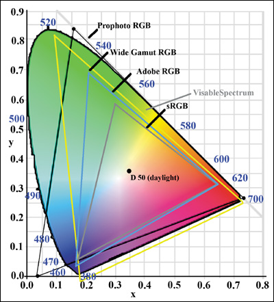
Before you begin working on Challen’s image, you need to have Photoshop set up for a non-destructive workflow. A non-destructive workflow is one in which you may do many manipulations without ever altering or losing the original file data. A typical non-destructive workflow starts when a RAW file is opened in the ProPhoto RGB color space in 16-bit. There is little or no clipping of colors in ProPhoto RGB (Figure 1.1.1), because it is such a large color space. It is the only color space that can contain all of the color that your DSLR can create. Files can always be converted later into smaller color spaces like sRGB (Figure 1.1.2) for display on the internet, but when a RAW file is opened in a smaller color space like Adobe RGB (Figure 1.1.3), colors that could have been printed had you used ProPhoto RGB are no longer in the file. Compare all of the color spaces in the visible spectrum in Figure 1.1.4.
Figure 1.1.1. ProPhoto color space

Figure 1.1.2. sRGB color space
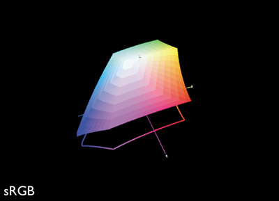
Figure 1.1.3. Adobe RGB (1998) color space
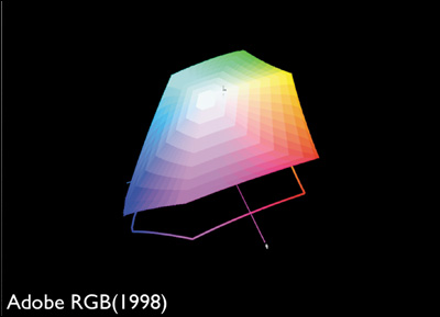
Figure 1.1.4. The visible spectrum and the three color spaces
Note
Once you capture in or convert into a smaller color space, all you have are the colors of that space. So if you have been converting your sRGB captured files into ProPhoto RGB thinking that you maximized the gamut of color, what you really have done is similar to pouring a quart of water into a gallon container; it is still only a quart of water.
Staying in 16-bit vs. 8-bit preserves all the tonal transitions in the RAW capture. Every time you adjust a file in Photoshop, Lightroom, Capture NX, or whatever RAW processor you choose, some information is lost. Staying in 16-bit guards against excessive information loss that could lead to posterization and banding. In the past, many photographers shied away from working in 16-bit due to large files sizes that slowed their workflow and were expensive to store. With dramatic improvements in computer processing power, coupled with equally dramatic decreases in the cost of storage, this is no longer the hurdle it once was. Non-destructive workflow ensures that any image editing can be undone, files stay in ProPhoto RGB 16-bit, and are saved in lossless formats such as .psd, .psb or .tif. Most importantly, this allows for the future growth and improvement of both technology and an individual’s technique. The reason for this revision is that, not only have the technologies available today improved, my understanding of how to exploit Photoshop has grown.
Set Up a Non-Destructive Workflow and Create a Custom Workspace
Step 1: Photoshop Preferences
Photoshop CS5 ships with a series of preset workspaces, any of which allow you to achieve a non-destructive workflow. I am going to tell you how to fine tune one of them, and then I will have you save this as a custom workspace. The reason for this is one of exit strategy; something you always want to afford yourself whenever you edit an image. You do this so that if anything happens to your settings, your computer crashes, or your menus get moved or closed, all you have to do is click on your custom workspace and you will be back in business.
- When you open Photoshop after you first install it, it defaults to the Essentials workspace. Go to the Window pull-down menu, select Workspace and then Photography (Figure 1.2.1).
Figure 1.2.1.

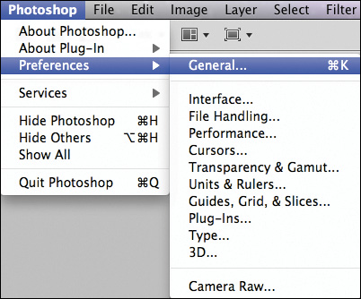
- Go to the Photoshop pull-down menu, select Preferences > General (Command + K for Mac / Control + K for Windows) (Figure 1.2.2) and the Photoshop Preferences dialog box will come up.
Figure 1.2.2.
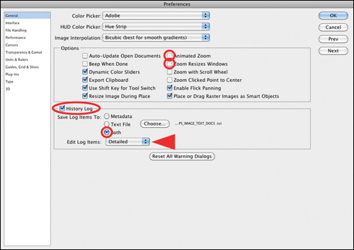
- In the General Settings box, leave the Color Picker set to Adobe, and Image Interpolation set to Bicubic. In the Options dialog box, turn off Animated Zoom.
- Next, click on the History Log and select Both. When the Save dialog box comes up, select New Folder and name that folder PS_IMAGE_TEXT_DOCS. Click Create and then Save in the Save dialog box (Figure 1.2.3).
Figure 1.2.3. Turning on the History Log
Note
I place the PS_IMAGE_TEXT_DOCS folder on the desktop. I also create a folder on the desktop bearing the name of the image on which I am working. Into this folder, I put a copy of the original RAW file, a copy of the modified RAW file, the layered .psd file, and any other files that I create related to that specific image. Make sure to name this folder so that it reflects the specific image to which all the files in it belong.
All of the choices I have had you make here are personal workflow choices. Although all of the features that I have had you turn off are well-executed pieces of code that are visually beautiful, I have disabled them because I find them visually distracting so they slow me down.
I find the History Log to be useful. (The older I get, the more useful I find it.) Its uses are twofold: you have a record of what you have done, which helps in figuring out the bill when you are doing work for someone else, and you have a written record of what you have done in case you want to replicate an effect. If you find you do not need the History Log, come back and turn it off—just be sure to save the changes in the custom workspace.
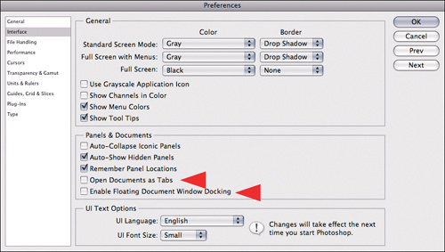
- Select Interface from the Preferences dialog box. In the General part of this dialog box, use the default settings. In the Panels & Documents part of the dialog box, however, turn off Open Documents as Tabs and Enable Floating Document Window Docking (both of these features make working with multiple images difficult and add unnecessary steps when you are engaging in an image harvesting workflow) (Figure 1.2.4).
Figure 1.2.4. Disabling the Open Documents as Tabs option
- Select Units & Rulers from the Preferences dialog box. Enter your unit preference (centimeters or inches) and, for new documents, I change the resolution to 360 ppi from 300ppi (Figure 1.2.5).
Figure 1.2.5. Setting the default resolution to 300ppi

Note
Because Epson printers, which I use, produce the best results at resolutions of either 240ppi or 360ppi, I select 360ppi. HP and Canon do best at 300ppi. This is because of the nature of the printer head technology. Epson uses Micro Piezo whereas HP and Canon use a thermal approach. The Epson head is far more accurate with regard to dot placement than either Canon or HP. I use primarily 360ppi because I do a lot of black and white images, and the majority of them are printed on Exhibition Fine Art paper, which is a glossy surface paper that holds dot structure better than any other paper I have used. I sometimes use a resolution of 240ppi when I am printing on fine art, cotton-based papers. This has to do with dot gain or the expansion of the ink dot due to the tooth of the paper.
- Click OK. You will now set up the next part of Photoshop for an Oz workflow.
Step 2: Setting Up Photoshop Color Space Preferences and File Bit Depth
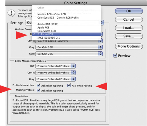
- Go to Edit > Color Settings (Command + Shift + K / Control + Shift + K). The Color Settings dialog box will come up. Its default is North American General Purpose.
- Select North American Prepress 2. In the Working Spaces part of the dialog box, click on the RGB pull-down menu and select ProPhoto RGB (Figure 1.3.1). Click OK.
Figure 1.3.1.
Note
You should do this so that all of the color space warnings are turned on. It is important to remember that once you assign a color space, unless the needs of image editing require that you go from a larger color space to a smaller one, you should use the color space of the file as it is.
Another reason to turn on the color space warnings is so that you are aware of any possible shifts in color that will happen when working with multiple images. Being aware of a possible color shift is important in case you need to address it.
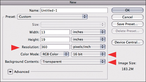
- Go to File > New File (Command + N / Control + N). Click on the Bit Depth pull-down menu and select 16 bit. For Background Contents, select Transparent (Figure 1.3.2), and leave the Width and Height at their default values. Click Save Preset, and then click OK in the New Document Preset dialog box. Click OK in the New File dialog box, and then click Command + W / Control + W to close the file that you just created.
Figure 1.3.2. Setting the New Document preset
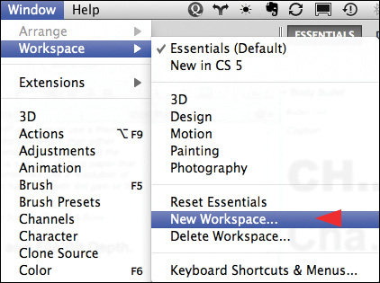
- Go to Window > Workspace > New Workspace... and save this workspace (Figure 1.3.3) in the New Workspace dialog box, naming it Workspace Oz2. Click Save.
Figure 1.3.3. Creating a New Workspace
Photoshop is now set up and optimized for photographic image editing.
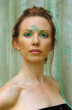
Practicing at Practicing: Image Maps
If a cluttered desk is the sign of a cluttered mind, what is the significance of a clean desk?
—Dr. Laurence J. Peter
Step 1: Using Image Maps
As an optical sensing device, the human eye scans a scene in a predictable sequence. It first goes to patterns it recognizes, then moves from areas of light to dark, high contrast to low contrast, high sharpness to low sharpness, in focus to blur (which is different than high to low sharpness), and high color saturation to low.
In order to make the viewer’s eye move across the image in a way that you decide it should, you must manipulate the light and dark areas, their contrast, their sharpness, their degree of focus or blur, and their saturation. So as not to feel overwhelmed when undertaking such a task, you should start by creating a list of the changes you would like to make. This is best done by creating an image map.
An image map is a Photoshop layer that sits on top of the image layer stack, on which you can make notes about what you are planning to do to an image. You can also use it to make notations on the various steps you will take, but what it does best is teach you how to create image-specific workflows. An image map is a planning device that helps you see the trees from the forest.
Note
You can download a tutorial QuickTime movie entitled “How to Make an Image Map” from www.welcome2oz.com (the same place you downloaded the source files for all of the lessons in this book). As I noted at the beginning of this chapter, image maps work best if you have a tablet or a pen-based display. Although it is possible to do everything in all the lessons in this book with a mouse, or even the trackpad of a laptop, you will be better served if you use a pen- or tablet-based system.
Keep in mind that image maps are designed to go away. They are the equivalent of training wheels. They are a good way to teach yourself how to organize and see, but you will not need them forever. To practice at practicing, you should do every lesson in this book with them and then again without them.
Another good reason to use image maps is that they allow you to make notes to yourself for retouching when you meet with a client. (I have the client sign the layer, so that there is a record in the file of what he wanted done and so there are no questions when I deliver the final image.) Image mapping also allows me to return to an image and note what I have done while it is still fresh in my mind so that I have accurate notes for the future.
Before you take the first “how to” step toward creating an image map, consider how believable you would like the finished image to appear. In this lesson, you do not want the viewer to know that you did any manipulation in Photoshop; you want to mimic what would have occurred had the model been properly lit in the first place.
A way to explain this can be found in Aristotle’s Poetics. In this work, he suggested that a believable improbability is better than an improbable believability. I believe this to be true and have extended this concept to define believable probability. What are these concepts and why are they important to digital photography?
The easiest way to understand these concepts is by using examples. Good examples of believable improbability are found in the Star Wars sagas. We do not travel faster than the speed of light, and walking, talking robots with feelings do not yet exist. In spite of this, we are willing to suspend disbelief, because the stories of love, longing, and conflict are believable even though they are improbable. In contrast, what follows is an example of improbable believability. I buy a lottery ticket in Los Angeles and the jackpot is $100,000. I win! The next day, I fly to New York City, buy another ticket, and win a jackpot of $75,000,000! The next day I fly to Chicago, repeat the process and win again! Although this could happen, you don’t believe it because it is so improbable.
The third concept, that of believable probability, can be explained using the Challen Cates image. You will create an image using Photoshop that the viewer will find both probable and believable, because the final image will be lit as though I had had the proper lighting equipment when I made the initial capture.
In order to assure that you create a believable probability rather than an improbable believability, you need to make sure that every choice you make in Photoshop leads to a result that will mimic the reality of proper lighting. For example, if you create a light that appears to shine from above, you need to create corresponding shadows that follow the direction of that light.
There will be images in which you will want to create a believable improbability. (There are some in this book. Try to identify them as you progress through the lessons.) The key to making something believable, no matter how improbable it may be, is to make sure that it conforms to the logic of our reality as much as possible. Once you have defined your goal for a particular image, you can begin to create image maps.
There are three free filter plug-ins from www.niksoftware.com/ozlessons: Tonal Contrast, Contrast Only, and Skylight filter. They will show up in your Filter pull-down menu under Nik Software as the Versace Edition. At the time of writing this book, the Nik Software filters only work in 32-bit in the Macintosh operating system; however, they work in 64-bit in Windows. Nik Software is in the process of updating them, but until then, Mac users will have to run CS5 in 32-bit. You do this by Control-clicking on the CS5 application icon. Select Get Info and click on the Open in 32-bit Mode checkbox. Close the window and start Photoshop.
You will also need to download the free copy of onOne Software’s FocalPoint 2.0 from www.ononesoftware.com/ozlessons. This is a fully functional version of the software and you will be a fully licensed user.
Lastly, once you have installed everything, if you are not working in the ProPhoto RGB color space, you need to set Photoshop to ProPhoto RGB. You do this by going to Edit > Color Setting (Command + Shift + K / Control + Shift + K) so that the Color Settings dialog box comes up. Select North American Prepress 2 in the Working Spaces in the RGB pull-down menu and, also, change the setting from Adobe RGB 1998 to ProPhoto RGB. Click OK.
Creating an Image Map
- Open the image “SHIBUMI_SOURCE_16BIT.tif” (located in the CHAPTER_01 folder that you downloaded from www.welcome2oz.com) in Photoshop.
Note
There is also a video on youtube.com where you can watch how I make an image map. The URL is http://www.youtube.com/watch?v=5ki3QhJkw-4.
Make sure that the image is in the neutral gray workspace by pressing the letter F. The gray space is best for making color decisions, because it gives you a color-neutral background. Gray is specifically used to minimize chromatic induction (visual color contamination), and a gray midtone is used to minimize contrast effects. By choosing a gray background, you can make the most informed decisions about changing the color, contrast, and shade of the image with which you are working.
- View the image in full screen (Command + 0 / Control + 0), and choose the Pencil tool from the tool bar (in the same place as the Brush tool). Double-click on the Set Foreground Color box in the Tools panel (the black and white squares located toward the bottom of the Tools panel). This brings up the Color Picker dialog box. Select a bright color. (I generally start with red and then work my way down on the color selector.)
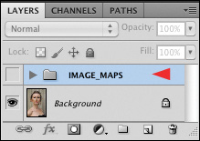
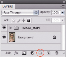
- Make sure the Layers panel is open, and click on the Create a New Layer Group icon (Figure 1.4.1). This will create a Layer Set folder in the Layers panel. Name the new layer set IMAGE_MAPS (Figure 1.4.2).
Figure 1.4.1. Create a New Layer Group icon
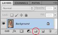
Figure 1.4.2. Creating the Layer set IMAGE_MAPS
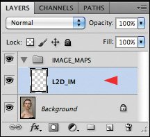
- Create a new layer by clicking on the Create a New Layer icon (Fig 1.4.3). Call the new layer L2D_IM (for Light-to-Dark image map) (Fig 1.4.4).
Figure 1.4.3. Create a New Layer icon
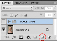
Figure 1.4.4. Renaming the layer L2D_IM
Note
At any level of expertise, giving your layers meaningful file names is an important part of creating an effective workflow. If many months after working on a file, you want to return to it to try a new technique, you will immediately grasp the purpose of each layer on which you originally worked and be able to retrieve the appropriate one on which to try your new approach. Perhaps you made a print or sent a file to a client, and changes are needed. Knowing at a glance what you did to the image will make life a lot easier should you have to go back and redo or undo something. It also makes your practicing at practicing sessions easier. If you get lost, you have an easily readable and retrievable road map.
- Select a brush size of 25 pixels. (You increase or diminish a brush’s size by pressing the square bracket keys, which are on the keyboard next to the letter P. Pressing the left bracket makes the brush smaller; pressing the right bracket makes it bigger.)
Note
Correct brush size is determined by the size and resolution of the image, so focus on the visual size of the brush, and not on its pixel size. For example, a 25-pixel brush would be much too large to use on a small, low-resolution image.
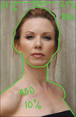
The Relationship of Light to Dark
For the first part of this lesson, I want you to manipulate the variables that I mentioned at the beginning of Step 1: light-to-dark, high-to-low contrast, and in-focus-to-blur. Remember, it is the person creating the image who decides the journey that the viewer’s eye will take. And it is that journey that causes the viewer to see the story you wanted to tell.
You control where the viewer’s eye will go by manipulating variables such as focus, light, and dark. I contend that when we view anything at all, there is both an unconscious and a conscious element involved. First, our unconscious eye, or the anatomical structure that makes up the eye, scans in the predictable manner I described above. Then, the conscious eye, the mind’s eye, interprets the image seen. It is how you control the unconscious eye that determines how the viewer interprets the image. This is a theme to which I will frequently return.
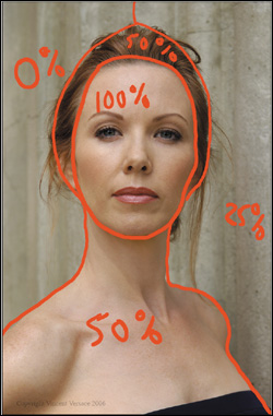
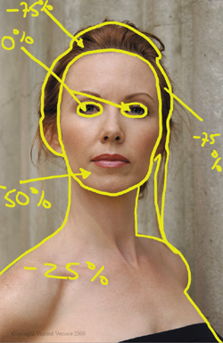
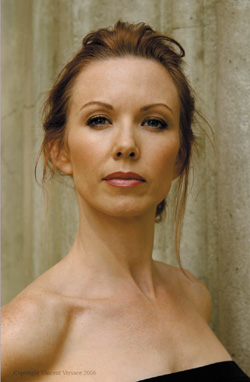
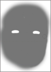
In general, I like to begin manipulating light-to-dark, thereby exploiting the unconscious eye’s tendency to move from light areas to dark ones. For this specific image, I want the viewer’s eye to go first to the face, then to the torso, then to the rest of the image.
You must first decide what ratio or relationship of light-to-dark to create within this image. I wanted the face to be brightest, so I set it at 100%. As light’s circle of illumination increases, its intensity diminishes, so set the hair and torso at 50%. The background should be darker than the face, hair, and torso. The light on the background should go from light to dark as the eye moves from right to left. (I will explain why in a moment.) Set the right side at 25% and the left side at 0%.
Note
As you create your image map, keep in mind that these percentages are just notations. You can change them any time. You are working from the global to the granular.
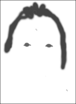
After those values are drawn on the L2D_IM layer, the image will look like this (Figure 1.5.1).
Figures 1.5.1 and 1.5.2. Light-to-dark image map, and Lighting image map
Placing Key and Fill Lights
If I had had all my lighting equipment at the photo shoot, I would have started by lighting the background, and I would have cross-lit it from left to right. Then I would have set key lights and fill lights. With a portrait, you usually want the viewer’s eye to go first to the subject’s eyes, so that is where you should put the key light. Then you might put fill lights on the lips and, to some degree, the torso.
Create a new layer and name it LIGHTING_IM (for Lighting image map). Pick a color other than red from the Tools panel to draw your lighting choices. (I chose blue.)
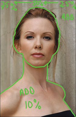
Here is the LIGHTING image map (Figure 1.5.2) showing the notation of the percentages I used: eyes: 100%, face: 50%, torso: 25%, and background areas: 50% and 25%.
The Illusion of Depth of Field
When shooting portraits, I find that a shallow depth of field (where only the subject is sharp and the background is out of focus) is visually pleasing. When you focus on the subject’s eye that is closest to the camera, the depth of field (the zone of acceptable sharpness) on the face will extend from the tip of the nose to a little past the ear. Generally that means shooting at f/5.6.
Create a new layer and name it D_OF_F (for Depth of Field), and pick a new color to use for your next set of image map notations (I chose light green) (Figure 1.5.3).
Figure 1.5.3. Depth of Field image map
In this case, the image was shot at f/6.3, with the model standing right against the wall, underneath the diffuser. The result is too much depth of field (DOF), with everything in focus, including the background.
Note
One of the issues that occurred during Challen’s photo shoot was that in order to evenly light her, I had to place her almost against the wall. I would have preferred that she be some distance away from and at an angle to it. In order to create this illusion in Photoshop, so as to achieve a believable probability, I had to create the correct quantity of in-focus-to-blur that would have occurred had I actually lit her properly and positioned her away from the wall. You also need to apply some degree of blur to her torso. (Since the point of focus is her eye, and one-third forward from that point should be in focus, the area in focus should stop at the tip of her nose. Any areas of her torso that extend past her nose should not be in focus.)
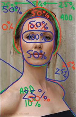
You now have a basic workflow to follow for manipulating the lighting and DOF of the Challen Cates image in Photoshop (Figure 1.5.4). (Keep in mind that the values I chose to use are only approximations and reflect relationships specific to this image.) Starting with a completely flat-lit photograph, you are now well on the way to creating a believable probability.
Figure 1.5.4. Combined image maps
Depth of field refers to the area that is in focus both in front and behind the true plane of focus. It has been shown that if the depth of the area that appears to be in focus in front of the true plane of focus is one foot, then the area that appears to be in focus behind the true plane of focus is two feet. This works out to a ratio of one-third in front in focus to two-thirds behind in focus; i.e. twice as much behind as in front.
The absolute distance that appears in focus depends on two factors: the size of the lens aperture and the distance from the camera to the subject. The larger the aperture, the “shallower” or smaller the area that is in focus. The smaller the aperture, the “deeper” or greater the area that is in focus. Additionally, the farther away a subject is from the camera, the greater its depth of field, i.e. the more that will be in focus. Conversely, the closer the subject is to the camera, the less its depth of field, i.e. the less that will be in focus.
In the lighting image map, we made some decisions as to where we would like the viewer’s eye to go: first to the face, then the torso, and then the background from right to left. The face and torso are easy to understand, but why right to left? Because we want to create the illusion that the model is farther from the background than she really is (Figure 1.5.3).
Figure 1.5.3.
Make the image maps invisible by clicking off the eyeball of the layer set IMAGE_MAPS. They will be out of the way, but available when needed.
Step 2: Correcting Digital Sensor Color Cast
Now that you have an image roadmap, working from the global to the granular, the next biggest issue is the correction of the image’s CCD/CMOS color cast. It is an important issue because it will affect all of the image editing choices you will make from this point on.
All RAW images, from any digital camera, exhibit some form of color cast as a result of the interpolation process that occurs when you bring that image into digital manipulation software such as Photoshop. The Challen Cates image on which you are working has a magenta/yellow haze.
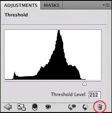
The most effective way to remove this type of color cast is to first define the black and white points of the image. Finding the white point is a bit more problematic than finding the black point—and finding a gray point is even more elusive—but you are going to find all three by using a Threshold adjustment layer.
There are some rules that are important to know when removing color cast caused by the interpolation of the data from a CCD/CMOS sensor. When looking for the black point, select your sample point from an area of “meaningful” black rather than using the first black pixel you see. If you select the very first black pixel that you see, it generally has RGB values that are R:0, G:0, and B:0. If no information was recorded, no color contamination exists. What you are looking for is a black pixel that has RGB information in it.
Finding a white point is completely different. You do not want to select a white point from an area of “meaningful” white. Rather, you want to find the pixels that are closest to pure white, without actually being pure white. (A pure white pixel will have RGB values of R:255, G:255, and B:255, which is of the same usefulness as a black pixel that has RGB values that are zero.) What makes finding a white point so problematic is that, much of the time, visible white and measurable white are two different things. (Measurable white, using the Threshold adjustment layer method, will always be biased to R:30%, G:60%, and B:10%, while visible white generally consists of equal values of RGB and tends to be a lot bluer than measurable white.) In addition, there are instances when there is no white point at all and, occasionally, there may be aspects of the white point color cast correction you may not like, i.e. you may actually like aspects of the color cast. For these reasons, it is a good idea to separate the black and white points into separate Curves adjustment layers, because it gives you options that you will see as this lesson progresses.
Note
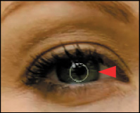
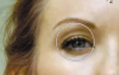
Looking at this image, visible white is found in the catch light of the subject’s eye.
Conceptually, it may be more accurate to view setting a white and black point as setting a light and dark one, because you do not want to use the pure white (R:255, G:255, and B:255) and pure black of an image (R:0, G:0, and B:0); you want to be as close as possible to those values without reaching them.
How to Find Black and White Points Using a Threshold Adjustment Layer
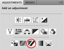
1. Make the background layer active. If you are working in CS4 or above, go to the Adjustments panel and select Threshold by clicking on the Threshold adjustment layer icon (Figure 1.6.1). (If you are working in CS3 or below, go to the bottom of the Layers panel, click on the Create a Fill or Adjustment Layer icon, and select Threshold.) A black-and-white representation of the image appears (Figure 1.6.2).
Figure 1.6.1. Threshold adjustment icon
Figures 1.6.2 and 1.6.3. Black and white image with Threshold adjustment applied, and whole image with first meaningful black
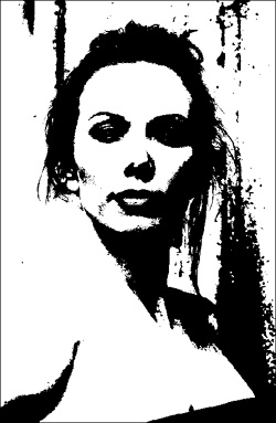
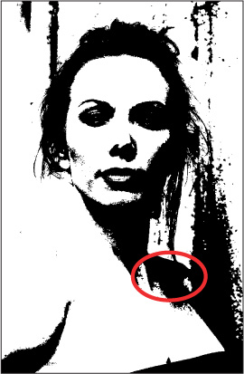
2. If you are working in CS4 or above, make sure that the Eyedropper tool is selected. (If you are working in CS3 or below, the tool is automatically selected.) Move the triangle slider (located at the bottom of the Threshold dialog box) to the left until the image goes completely white. As you move the slider slowly back toward the right, you will see image detail start to emerge in black. The first meaningful area of black that you see is where you should take your black sample point (Figures 1.6.3). (Meaningful black is an area in which you can see “something.”)
3. Choose a black point from the top of the model’s dress by zooming into this area (Command + Space / Control + Space gives you the Zoom tool) and then by Shift-clicking a sample point (Figures 1.6.4).
Figure 1.6.4.
4. Bring the image back to full screen (Command + 0 / Control + 0), and move the triangle slider all the way to the right. The image will be completely black, but you should see a sample point (your black point) bearing the number 1 in the lower right corner.
Note
Even though you see “meaningful” black in areas of the model’s hair and eyes, I chose to put my black point in the model’s dress, because her dress was actually black. You will notice, however, that the dress’s color recorded as dark blue.
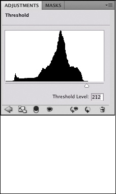
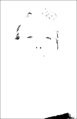
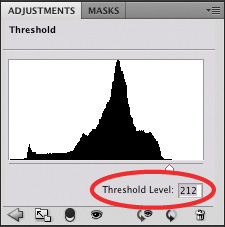
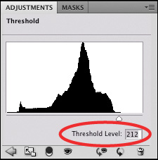
5. Move the slider slowly back to the left until the first area of white pixels appear. (I saw this at a Threshold level of 212.) (Figures 1.6.5)
Figure 1.6.5.
Note
When choosing a potential white point, get as close as you can to the first white pixel that you see. If that pixel has an RGB value of R:255, G:255, and B:255, just like the a black point that has a RGB value of 0,0,0, it contains nothing to measure. This is why you should get as close as you can to the first white pixel without actually selecting it. To remove a color cast, you must have a pixel that has a variation between the red, green, and blue pixel values.
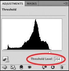
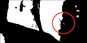
6. The three areas that come up are on Challen’s shoulder, cheek, and forehead. Move the slider to the right so that it is at the very end of the black in the histogram shown in the Threshold dialog box. (For this image, that is a threshold level of 204.) What you should now see is one white square in a field of black (Figures 1.6.6 and 1.6.7).
Figure 1.6.6.
Figures 1.6.7 and 1.6.8. Three areas of white in Threshold preview, Sample point 2 placed on the white pixels
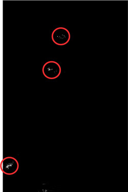
7. Zoom into the area of the white squares above her shoulder. One of these three white squares is going to become your white point. You are going to further define your white point by moving the threshold level upward. Click on the white triangle and slowly move it until only one white square remains, which occurs in this image at a threshold level of 207. Make sure the Eyedropper is selected in the tool bar. Shift-click on the white square, and you should see a sample point appear with the number 2 (Figure 1.6.8).
Finding a “Sometimes” Midpoint Using a Threshold Adjustment Layer
Contained within every image is a set of numbers (RGB values) that corresponds with the always-difficult-to-find midpoint value. What follows is the easier of the two ways to find that midpoint; the one that works when the image has easy-to-find neutrals. (Later in this book, you will learn how to find a midpoint value even when you cannot see one.) The concrete wall behind Challen is made up of neutral tones that lend themselves to finding a useful midpoint.
8. Bring the image back to full screen (Command + 0 / Control + 0), and move the triangle slider until the Threshold Level is at 128 (Figures 1.6.9 and 1.6.10). When you turn the Preview Eyeball off on the Threshold adjustment layer located at the bottom of the dialog box, you will see a red line through the Eyeballs. (In Photoshop CS3 and below, click off Preview.)
Figure 1.6.9. The image at a Threshold of 128

Figure 1.6.10. The Threshold adjustment set to 128
9. Zoom into the model’s right shoulder containing the desired neutral values (Figure 1.6.11).
Figure 1.6.11. Zoom into the shoulder
10. Click on the Preview Eyeball of the Threshold adjustment layer. In the Threshold, type 127, and press Return. Command + Z / Control + Z back and forth, and observe where black pixels appear and reappear on the wall. Once you have found an area like this, zoom into it. Repeat toggling back and forth between a threshold level of 127 and 128, and watch where the pixels appear and reappear. When you return to a threshold level of 128, pick a single pixel that reappears, and place your third sample point (Figure 1.6.12).
Figure 1.6.12. The third sample point
11. Click the Trash Can icon (Figure 1.6.13) to discard the Threshold adjustment layer (or select Cancel in the Threshold dialog box if you are working with CS3 or below). This layer was needed only to help you locate the potential white, mid- and black points.
Figure 1.6.13. Discarding the adjustment
Living in the Land of 2%
Whenever you work on an image, regardless of the RAW processor you use, you clip data that results in the introduction of artifacts. It is extremely important to understand that such artifacting is cumulative and can become multiplicative. Furthermore, the image data that you see when you first open a RAW file (before you do anything to it) is the cleanest it will ever be.
When you decide to manipulate your file, you must decide whether or not to live in the land of 2%. If editing an image brings it 2% closer to your original vision, you must do it, and thus, you are living in the land of 2%. To paraphrase Viola Spolin (internationally renowned theater educator, director, and actress), the moment you decide something in the creation of your work doesn’t matter, is the moment you decide that your work doesn’t matter. I believe that everything you do must matter. What becomes your greatest challenge is editing your image so as to remove only those things that are not compatible with your original vision in such a way that you create the smallest amount of artifact possible.
Why and how I do many of the things I do is because I want my image to be 2% closer to my original vision, but I do not want to cause a possible 15–20% quality decrease in my image file due to the cumulative and potentially multiplicative aspects of artifacting. Everything I do is in service of the print, which is in service of my vision, or voice, and I want my voice heard and my vision seen without any detractions.
That brings me to another thought. I have been talking about correcting a digital file’s color cast, but not all color cast is objectionable, and sometimes, it may merely be aspects of the color cast you do not like.
This is what I know:
- All images have a color cast.
- The color cast may be objectionable, or merely aspects of the color cast are objectionable.
- Aspects of color cast may be usable.
- The untouched file is the cleanest it will ever be.
- Anything I do to this file clips data and introduces artifacts.
- All artifacting is cumulative and may be multiplicative.
- When working on a image, I want to clip as little data as possible.
- I want the greatest image control I can get.
- I always want to be able to undo what I have done.
I want you to apply these thoughts to the task at hand, which is removing the color cast of this image, while sparing the loss of information and maintaining the greatest amount of aesthetic control possible. You will do this is by using separate Curves adjustment layers for setting this image’s white point, black point, and midpoint. Because you will make one adjustment per layer, you will minimize the artifacts that you will introduce.
Since I adhere to Albert Einstein’s tenet that we should make things as simple as possible and no simpler, why would I want you to use three separate Curves adjustment layers when it would be simpler to do the three points on just one? The reason is that the resultant images are profoundly different. This is what the image looks like when I separate out the black, mid-, and white points onto three separate Curves adjustment layers (Figure 1.7.1), and this is what it looks like when I do the three points in just one (Figure 1.7.2).
Figures 1.7.1 and 1.7.2. Comparing the effect of three separate curves adjustments (left) with one (right)
Another reason to use three separate curves is that if you combine the three points into one Curves adjustment layer, you lose control over your image. You cannot return to the image (should you decide or need to) to brush things backward, change opacities, or re-blend the colors. Some photographers use one layer to save space on their hard drive and to simplify their workflow. The result, however, is that they are stuck with what they have done. Trying to make something simpler than it should be can cause many unanticipated problems.
Another benefit of this approach is that you can control the amount of whatever effect you are using: globally through the use of the layer’s opacity (in the Layers panel), and selectively through the use of layer masks for each of the adjustment layers.
Using Multiple Curves Adjustment Layers to Remove Color Cast
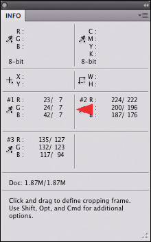
In Step 11, under finding a midpoint, you discarded the Threshold adjustment layer. After doing that, the image reappeared in color displaying the three sample points you created: one on the model’s cheek, one on the concrete wall, and one on her dress. The series of numbers that appear in the Info panel are the actual color values of each of those points. (Sample point 1—your black point: R:18, G:31, and B:17; Sample point 2—your white point: R:219, G:192, and B:208; and Sample Point 3—your midpoint: R:131, G:129, and B:114.)
Note
In CS3 and below, click Cancel to get rid of the Threshold adjustment layer. In CS4 and above, click on the trash can. Be aware, however, that in CS4 and above, if you are using actions or Extension panels, you click Cancel the same way you would if you were using CS3 and below.
If your numbers do not exactly match mine, it simply means that we picked slightly different sample points. Notice that the area you clicked on for your white point was not located in the area of the eye. In this instance, visible white is different from measurable white. For the purpose of demonstration, I placed a white sample point (and named it Sample Point 4) in the specular highlight of the eye. This is the whitest, visible white point in the image.
- Make sure the Layers panel is open, and click on the Create a New Layer Group icon (Figure 1.8.1). This will create a Layer Set folder in the Layers panel. Name the new layer set BP/WP/MP.
Figure 1.8.1. Create a New Layer Group icon
- Making sure that you are in the BP/WP/MP layer set and turn Caps Lock on; the pointer becomes the crosshairs cursor. If you are in CS3 or below, go to the bottom of the Layers panel, and click on the Create New Fill or Adjustment Layer radial button. (It is the third radial button from the left and is a half-white, half-black circle). Select Curves from the fly-out menu. You will now create the first of three Curves adjustment layers. If you are in CS4 or above, you can either create a Curves adjustment layer this way or you can use the Adjustment panel.
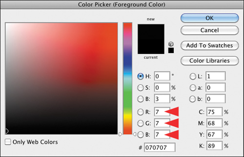
- When the Curves dialog box comes up, click the black eyedropper to set the threshold at which you want the black eyedropper to sample (Figure 1.8.2). Now, double-click on the black eyedropper that is located in the lower right corner of the dialog box. The Color Picker dialog box will come up. In the RGB values part of the dialog box, type 7 in the R, 7 in the G, and 7 in the B. Click OK (Figure 1.8.3).
Figure 1.8.2. The black eyedropper in the Curves adjustment
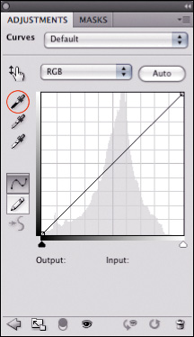
Figure 1.8.3. Setting new values for the black eyedropper
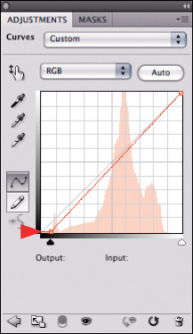
- Zoom into the area of sample point 1. Select the black eyedropper, which is the leftmost eyedropper of the three in the Curves adjustment layer dialog box, and you will see a circle with two crosshairs. Line the crosshairs up until it appears that there is only one, and click. Notice how the color changes (Figures 1.8.4 and 1.8.5).
Figures 1.8.4 and 1.8.5. Before the BP Curves adjustment and after the BP Curves adjustment

Note
The RGB values of R:7, G:7, B:7 approximate the beginning of what is known as Zone II (textured black) in the Zone system, as developed by Ansel Adams and Minor White. For further discussion of the Zone System, see The Zone System Manual by Minor White.
When you define the white point, you will set the white point eyedropper for the upper end of Zone IX (textured white), because in a fine art print, you are looking for 100% ink coverage in the highlights (no place where the paper shows through the ink) and shadows that have detail throughout. In other words, you want no paper showing and no ink wasted.
If Photoshop asks, “Want to save the new target colors as default?” click Yes for both the black and white point curves.
Because you are addressing issues of color (color cast), you are going to leave the blend mode of this Curves adjustment layer, as well as the one you are about to create, as Normal.
You will now see that, in the Info panel, sample point 1 has changed from values of R:19, G:17, and B:31 to values of R:9, G:9, and B:9. Your next task is to fine tune each of the RGB channels in your Curves adjustment layer to R:7, G:7, and B:7 (Figure 1.8.6). In so doing, you will recover some more data that may be potentially clipped in the course of removing color cast, as well as to remove the color cast from the black aspect of your image.
Figure 1.8.6. Equal RGB values for the black point
- From the Modify Individual Channels pull-down menu, select the Red channel and click on the anchor point at the bottom of the channel (Figures 1.8.7 and 1.8.8). Using the directional arrows on your keyboard (for this image, it is the right arrow), move the anchor point to the right until the number in the Info panel moves from 9 to 7. (For me, it was 2 clicks for all three channels.) Repeat this process for the green and blue channels. In the Info panel, all the RGB values should now equal 7. By redefining the black point, you have also removed the CCD/CMOS color cast from the black parts of the image (Figures 1.8.9 and 1.8.10). In the Layers panel, name this layer BP (for Black Point) and turn its eyeball off. You should repeat this process for the white and midpoints.
Figure 1.8.7. Selecting the Red channel
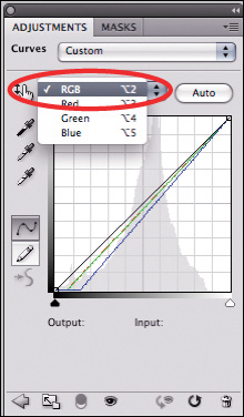
Figure 1.8.8. Fine tuning the anchor point
Figures 1.8.9 and 1.8.10. Before the BP Curves adjustment and after fine tuning the BP Curves adjustment


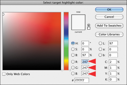
- Repeat the steps for creating a Curves adjustment layer. To set the threshold of the white eyedropper, select the white eyedropper, double-click on the white eyedropper and set the RGB values to R:247, G:247, and B:247. (This approximates the upper end of Zone IX) (Figure 1.8.11). Click OK. Zoom into the area of sample point 2, align the crosshairs, click, and then click OK. You have set the white point. In the Info panel, sample point 2 (the white point) should have changed from R:219, G:208, and B:192 to R:247, G:247, and B:247.
Figure 1.8.11. Setting the new white point values
- From the Modify Individual Channels pull-down menu, select the Red channel, and click on the anchor point at the top of the channel. Using the directional arrows on your keyboard (the right arrow for this image), move the anchor point to the right until the number in the Info panel moves from 253 to 247. (For me, it was 5 clicks to the right.) Repeat this process for the green and blue channels. (For me, the green channel was 5 clicks to the right, and the blue was 7 clicks to the left.) The RGB values in the Info panel should now equal 247 (Figure 1.8.12). In the Layers panel, name this layer WP (for White Point) and turn its eyeball off. Compare before (Figure 1.8.13) and after (Figure 1.8.14).
Figure 1.8.12.
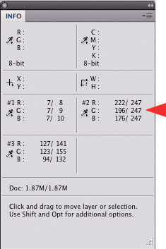
Figure 1.8.13. Before the WP adjustment

Figure 1.8.14. After the WP adjustment
- For the last time, repeat the steps for creating a Curves adjustment layer. Select the Set Graypoint eyedropper. (Do not worry about double-clicking on the gray-point eyedropper; the RGB values are already set to R:128, G:128, and B:128.) Zoom into the area of sample point 3, align the crosshairs, click, and then click OK. You have set the midpoint or gray point. The Info panel for sample point 3 should have changed from R:131, G:129, and B:114 to R:124, G:124, and B:124.
- Once again, from the Modify Individual Channels pull-down menu, select the Red channel and click on the anchor point in the middle of the channel. Using the directional arrows on your keyboard (the left arrow for this image), move the anchor point to the left until the number in the Info panel moves from 124 to 128. (For me, it was 4 clicks to the left.) Repeat this process for the green and blue channels. (For me, the green and blue channels were both 4 clicks to the left.) The RGB values in the Info panel should now equal 128. In the Layers panel, name this layer MP (for Midpoint). Compare before the MP adjustment (Figure 1.8.15) and after (Figure 1.8.16).
Figures 1.8.15 and 1.8.16. Before and after the MP adjustment


- Now that you have dialed in each of the three correction curves, turn on the eyes of the BP and MP Curves adjustment layers. With all the layers on, the image should look like this: before and after (Figures 1.8.17 and 1.8.18).
Figures 1.8.17 and 1.8.18. Before and after the CCD/CMOS color correction
You have successfully removed the CCD/CMOS color cast from the white, mid, and black aspects of the image, thereby eliminating the color contamination inherent in the process of converting RAW files to any usable file format.
Making Lemonade from Lemons: Selectively Using File Color Cast to Your Advantage
When you create images that reflect your vision of the world, the only rule is that there are no rules. No one cares what you did to the image to make it look the way it does; they care only that your image moves them. The viewer wants so much to believe in your image that he or she is willing to suspend all disbelief to take the journey. What viewers do not want to see are the chalk marks of your post-processing, for if those are evident, their willing suspension of disbelief ceases. So when your image has some lemons, make lemonade; just do it so that no one can see the peels.
When trying to create a believable probability, you need to pay attention to the way people naturally perceive things. For example, painters are taught that warm colors appear to move forward in an image while cool colors move backwards. What is true for them is also true for photographers, which means that the closer an object is to the camera, the more warm, or yellow and red, it will appear. If the object is further away, it will appear cool or blue. Also, shadows tend to be bluer or cooler than areas that are lit, which tend to be warm. What this means is that if you are trying to create the illusion of DOF in the Challen image, in addition to making her look like she was lit with appropriate lights, you need to pay attention to the colors of things. (That attention needs to be paid from the very moment you open the file and choose to change something, because everything you do must be about minimizing artifact. You must also endeavor to create a workflow that makes things as simple as possible, but no simpler.)
One of the reasons that I wanted you to separate the black, white, and midpoint color cast corrections is so that you can have complete control over the colors of all objects in any of your images. You may decide that you want to use all three color cast corrections, but you may want to use just one or two, or none at all. You may also want to change the order of your three correction curves, as well as the individual opacities of each layer. Lastly, you may choose to selectively adjust the color of one or more of the smallest of areas by using layer masks. So even though all files you capture have varying levels of color cast, you will be able to use any part of that cast to your advantage.
Looking Before You Leap
Before you move on and do any brushwork, assess each of your color cast correction layers for what you do and do not like about each. At each point along the way to creating an image, you should re-evaluate what you have already done.
My first observation when I re-evaluate this image is that I do not like the overall color cast before correction. I do not, however, like the coolness of the image once the color cast is removed. I do like some of the warmth of the black point correction, but I do not like what it does to Challen’s eyes and hair. I like the overall effect of the white point correction, but not what it does to her face and hair. I like aspects of the original, uncorrected image, specifically the tones of her hair, and I am happy with the midpoint correction. With all these observations in mind, here are the first image maps that I drew: black point correction brush back (Figure 1.9.1) and white point correction brush back (Figure 1.9.2).
Figures 1.9.1 and 1.9.2. Black point correction brush back image map and white point correction brush back image map

Fine Tuning the Color Cast on the Curves Adjustment Layers to Set the Stage for the Creation of the Illusion of Depth of Field
With the global color correction behind you, the granular color correction is next. Begin by thinking through what steps you want to take.
I chose to begin on the BP and to brush back the model’s eyes in this layer, because there are aspects here that I like. Look at this before the black point correction (Figure 1.9.3) and after (Figure 1.9.4).
Figures 1.9.3 and 1.9.4. Before and after the BP adjustment

Then, look at the image before the white point correction (Figure 1.9.3) and after (Figure 1.9.5), and you can see that this correction cools the image and removes some of the color cast from her hair.
Figures 1.9.3 and 1.9.5. Before and after WP adjustment

If you look at the image before the midpoint correction (Figure 1.9.3), and then after (Figure 1.9.6), the image is even cooler than it was before you did the midpoint correction. When you put all three together, you get what the image looked like when I shot it, but it is not yet what I want it to become. Look at the image before the correction (Figure 1.9.3) and after the black, white and midpoint corrections (Figure 1.9.7).
Figures 1.9.3 and 1.9.6. Before and after MP adjustment

Figure 1.9.3. Before any corrections
Figure 1.9.7. After all corrections
In order to make this image match my initial vision of it, I must create the illusion of DOF. In order to do this, you will use color to your advantage. Since you now know that warm colors appear to move forward in an image, and cool colors appear to recede, if you make Challen’s face the warmest part of the image, her body the second warmest, and the background the coolest, you will begin to create the illusion that there is a greater separation of Challen from the background than there really was.
There are many things that you could do to this image to affect its color cast. You could individually look at the black, the white, or the midpoint; you could put them together as seen in Figure 1.9.7, or you could lower the opacity of each of the layers. But what I would like you to do, after looking at this Black point brush back image map (Figure 1.9.1), is to brush back the areas that I have drawn in and keep the areas with no notations: that means brushing back the pupils of her eyes, brushing back the whites of her eyes, and then her hair.
Finding the Gray Areas: Step 1: Fine Tuning the Black Point Curves Adjustment Layer
- Turn off the Black Point image map, and zoom into Challen’s face and hair. Make the layer mask active on the Black Point (BP) Curves adjustment layer.
- Select the Brush tool (keyboard shortcut B), and zoom in to her face. Set the opacity to 50% by pressing 5.
- Start with her eyes. Select the Brush tool (making sure that Caps Lock is off) and shrink it until it is just a bit smaller than her eye (Figure 1.10.1).
Figures 1.10.1. Setting the brush size
- Make sure that the foreground color is black. (Use the keyboard shortcut D to reset the foreground and background color. To reverse the foreground and background color, use the keyboard shortcut X.) You will paint with black, because the layer mask is white. Black conceals, white reveals. (See the sidebar Unmasking Layer Masks and the 80/20 Rule.) Start by brushing just the pupil of her eye.
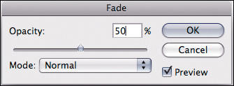
- Bring up the Fade effect tool by using keyboard Command + Shift + F / Control + Shift + F (Figure 1.10.2) or go to the Edit menu. Look at the effect at more than 50% (Figure 1.10.3) and at less than 50% (Figure 1.10.4). I selected 69% (Figure 1.10.5) because I liked concealing more of the correction. Click OK.
Figures 1.10.2. Fade effect dialog box
Figures 1.10.3. Fade set to more than 50%
Figures 1.10.4. Fade set to less than 50%
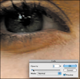
Figures 1.10.5. Fade set to 69%
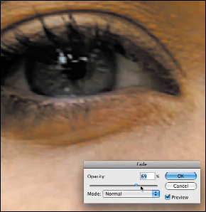
- Hold the space bar down to bring up the Move tool and move the image over to her right eye (Figure 1.10.6). Brush over her right pupil as you did on her left eye. Next, bring up the Fade effect tool (Command + Shift + F / Control+ Shift + F). Type in 69% and click OK. You know it is going to be 69%, because it was 69% on her left eye and they should match (Figure 1.10.7).
Figure 1.10.6. Move to her right eye
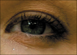
Figure 1.10.7. Fade the brushwork to 69%
- Shrink the brush size by using the bracket keys located next to the letter P. The left bracket key makes the brush smaller, while the right bracket key makes it larger. The brush should fit in the area where her tear duct and her eyelid meet (about 20 pixels) (Figure 1.10.8).
Figure 1.10.8. Shrinking the brush size again

- Brush in the whites of her eyes at 50%.
Note
Although there is an unwanted overlap in the layer mask from inadvertently brushing over the same area, this is easily corrected. (See the sidebar Error-Free Layer Masks.)
- Once you have fixed the layer mask using one of the techniques discussed in the Error-Free Layer Masks sidebar (Approach 1 is the best choice for this image), use keyboard command D to reset the foreground and background colors to black and white. Next, select a brush opacity of 50%. (Keyboard shortcut 5 gives you an opacity of 50%.)
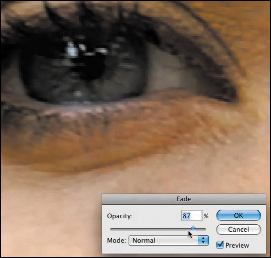
- Zoom out so that Challen’s face fills the screen. Using the right bracket key, increase the brush size to 90 pixels and brush back all of Challen’s hair. After that, bring up the Fade effect dialog box (Command + Shift + F / Control + Shift + F), and set it to 81% using the slider. Compare the before (Figure 1.10.9), and after (Figure 1.10.10), and look at the image map (Figure 1.10.11) and the final layer mask (Figure 1.10.12).
Figure 1.10.9. Before the brushback

Figure 1.10.10. After the brushback
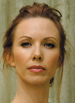
Figure 1.10.11. The brushback image map
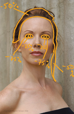
Figure 1.10.12. The resulting layer mask
Note
You do not have to be precise with the layer mask, because you can later return to and refine it using one of the approaches discussed in the Error-Free Layer Masks sidebar. Also, located at www.welcome2oz.com, there is a QuickTime presentation that you can watch on how to do this. Simply go to the source files for this lesson.
- Once you have brushed Challen’s hair back, Option- / Alt-click on the layer mask to display it. With the Brush tool still selected, set its opacity to 100% (keyboard shortcut 0). Then, Option- / Alt-click on the gray part of the mask. (Option- / Alt-clicking on a layer mask brings up the sample eyedropper.)
A Faster Layer and a More Accurate, Error-Free, Masking Workflow
Before you go further, I want to tell you how you can avoid some of the problems that can arise when you re-brush. In my opinion, the only way to find the right amount of gray for which you are looking is through the use of opacity. However, depending on whether the layer mask on which you are working is filled with black (for concealing the effect) or with white (for revealing the effect), using opacity may be problematic when you are trying to refine a layer mask created by using varying opacities of white and black. (See the 80/20 Rule sidebar.) The reason is that if I brushed on my layer mask at 50% and missed a spot that I later touched up and that overlaps my original brushing, that overlap would now be at 75%. (Fifty percent of fifty percent is twenty-five percent.) Just because my color may appear to be 50% gray, it is really still black. At 50% opacity, however, it will produce a 50% gray. So if I re-brush over anything on which I have already worked, it will be as if I was brushing at 75%. The outcome is the creation of a halo that is both undesirable and visible in the final image. If, however, I go to 100% opacity, and sample and paint with the grays that I created, I get to have my creative cake and eat it too. I no longer have to worry about creating halos, because all I am doing is painting with the same color gray that surrounds the area I originally missed. When you tightened up the eye aspect of this layer mask, you got a little taste of how useful this technique can be.
- Click on 0 (zero) to set the brush opacity to 100% opacity. Option- / Alt-click on the gray part of the layer mask. (Holding down the Option / Alt on a layer mask brings up the sample eyedropper. Clicking on it while holding down the Option / Alt key samples the color.) In the Tools panel, the color gray will show up in the foreground box. Brush in the white area and touch it up. The beauty of this approach is that it does not matter how many times you paint over the same area, because it is the same density of gray as the area that you sampled.
- Another advantage of working this way, is that once you have established the amount of density you want for Challen’s hair, you can keep painting with the same color, and you will get the same density of gray in your layer mask in those areas in which you have not yet done brushwork. Brush in the rest of the area that you mapped in your image map. Look at the layer mask and the image after refining the layer mask (Figures 1.10.13 and 1.10.14).
Figure 1.10.13. Refined layer mask
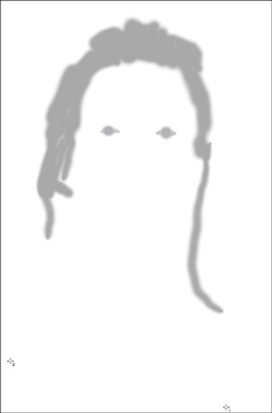
Figure 1.10.14. The image after refining the layer mask
You have completed fine tuning the Black Point Curves adjustment layer. Next, you will turn your attention to fine tuning the White Point Curves adjustment layer.
Figure 1.11.1. Before
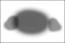
Figure 1.11.2. After
Now that you have a layer mask, this is the way to have one that has no missed areas or unwanted overlaps.
As I discussed in the 80/20 Rule, when you are working on a layer mask, you are working in grayscale. This means that when you change the opacity of white or black (depending on whether you are revealing or concealing), you are changing the density of the color with which you are working. That change in density manifests itself as shades of gray on the layer mask.
When you are working with opacity on a layer mask, you might miss an area. Because brushing is cumulative, it is almost impossible to match up the areas you missed with the areas that you didn’t. Rather than try the conventional approach to brushing, treat the layer mask as a color: the color gray.
Approach 1: Make the layer mask visible at full screen (see the Being in Two Places at Once section of the previous sidebar), and make the layer mask active. Select the Brush tool and set the brush opacity at 100%. Option- / Alt-click on the area that you want to sample (the Option / Alt key brings up the sample tool eyedropper when you are in the Brush tool), and brush over the area you missed or in which you have an unwanted overlap. (Remember, you are painting with gray.)
Approach 2: Set the brush opacity to 100%. Option- / Alt-click on the area that you want to sample. Select the Polygonal lasso tool. (The keyboard command is the letter L. If you want to scroll through any tool set, hold down the Shift key and click on the tool’s letter until the desired tool appears.) Click around the area and, when you have the desired area selected, Option + Delete / Alt + Backspace to fill with the foreground color.
Approach 3: (The Peter Bauer Method)
- In order to make the layer (rather than the mask) active, click on the layer thumbnail to the left in the Layers panel.
- Layer > Layer Style > Stroke. (Use the default color of red unless the image has a lot of red in it.) Increase the stroke width to 10 or 15 pixels.
- Click OK in the Layer Style dialog box.
- Click on the layer mask thumbnail to the right in the Layers panel.
- Where you see blobs of red in the image, there are stray black or white areas, so (with the layer mask active) simply paint over the red spots with the appropriate color and watch them go away.
- After cleaning up the mask, delete (or hide) the Stroke layer style.
Step 2: Fine Tuning the White Point Curves Adjustment Layer
It is time to address the remaining granular adjustments of the white point. Before you begin, look at the White Point Brush Back image map before the adjustment (Figure 1.12.1), as well as the image map after the white point correction (Figure 1.12.2). Also, review the image before and after without the image map (Figures 1.12.3 and 1.12.4).
Figure 1.12.1. WP Brush Back image map before the correction
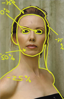
Figure 1.12.2. The same image map after the WP correction
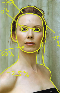
Figure 1.12.3. Before the WP correction
Figures 1.12.4. After the WP correction

When the white point correction is applied, the image cools down. In Challen’s image, you are trying to create the illusion of DOF, as well as create the illusion that the image was actually lit with hot lights. While doing this, you must ensure that you stay as close as you can to the original file. With this in mind, look at the original image map.
I suggest leaving her eyes alone, but brushing about 75% of the white point correction back into her hair, 25% into her body, and 50% into her face. This allows more of the image’s warmth to bleed through. (Warm colors appear to move forward in an image and cool colors recede, so the background in this image appears to be further away than it actually was.)
- Make sure that the White Point Layer Mask is the active layer. Select the Brush tool (keyboard shortcut B) and make sure that the foreground color is black and the background color is white (keyboard shortcut D). Set the brush opacity to 50% (keyboard shortcut 5) and make your brush is about the size of Challen’s eye socket, which is about 300 pixels (Figure 1.12.5).
Figure 1.12.5. Adjusting the brush size
- Brush in the whole area of her face. (At this moment, disregard her eyes.) Compare before the brushwork (Figure 1.12.4) and after brushwork (Figure 1.12.6).
Figure 1.12.4. Before the brushwork

Figure 1.12.6. After the brushwork
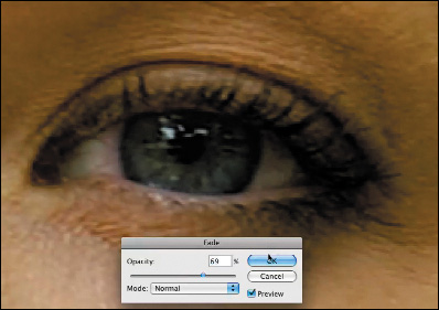
- Bring up the Fade effect dialog box (Command + Shift + F / Control + Shift + F). Move the slider first to the left, and then to the right to see if you want less or more effect. For this image, I chose 63%. Click OK. Compare before the brushwork (Figure 1.12.4) and after (Figure 1.12.7).
Figure 1.12.4. Before the brushwork
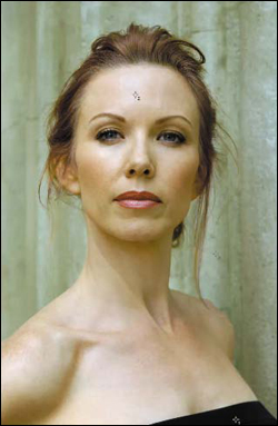
Figure 1.12.7. After brushwork on her face

- Next, zoom into her eyes by holding down the Command + Space / Control + Space keys and, starting at the upper left part of her face, just above her eyebrow, drag the magnifying glass (in Windows it is a white dot with a + in it) to the lower right part of her face, just under her eye (Figures 1.12.8).
Figure 1.12.8. Focusing on her eyes
- Press the D key, for default (the foreground color is black and the background white), and then the X key (to switch the foreground and background colors), so that you have the foreground color in white. Press the number 0 to set the brush opacity to 100%. Click the left bracket key and set the brush size to 40 pixels. Brush back just Challen’s eyes, specifically their whites and her pupils, and take a look at the layer mask (Figures 1.12.9 and 1.12.10).
Figure 1.12.9. The eyes afer cleaning up the brushwork
Figure 1.12.10. The layer mask
Note
I did the adjustment described above in this manner, because is it is easier to brush back the smaller area than it is to work around it. I always work from the global to the granular.
- Bring the image back to full screen (Command + 0 / Control + 0) and look at your layer mask. You still need to do brushwork on her body and hair. Set your brush to an opacity of 50% (keyboard command 5). Increasing the size of your brush to a diameter of 200 pixels (right bracket key), brush just the outline of her body, and a little in its center. (Again, it is not yet important to be exact.) Bring up the Fade effect dialog (Command + Shift + F / Control + Shift + F) and move the slider left and right to see if you want more or less of the effect. In this case, I chose 32%.
- Option- / Alt-click on the White Point Layer Mask (Figure 1.12.11) and then on the light gray area of Challen’s chest (the area in which you just brushed) to sample the color (Figure 1.12.12). Press the number 0 to set the brush to 100% opacity, and brush in the areas that were missed, tightening up the edges as you go (Figure 1.12.13). This is the quickest, most efficient way that I know to make a layer mask.
Figure 1.12.11.
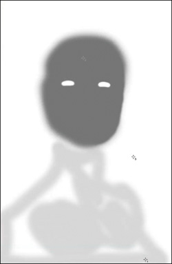
Figure 1.12.12. Sampling the gray
Figure 1.12.13. The final layer mask
- Next, take care of her hair. Click on the forward slash key (located next to the right bracket key) to bring the image back with the image map layer visible. The White Point layer should still be active, as should the layer mask. Click on the D key to set the foreground/background colors to default, and then click the X key to switch the colors. (The foreground should be black and the background white in the Tools dialog box.) Click the 5 key to set the opacity to 50%, and then the B key for Brush, making sure your layer mask is active. Now paint Challen’s hair according to what you mapped. Once that is done, bring up the Fade effect dialog box (Command + Shift + F / Control + Shift + F) moving the slider right and left to see if you want more or less of the effect. In this case, I chose 50% more. Also, I chose 88% opacity for this part of the image brush back.
- Zoom into the tendrils of her hair on the right side of the image (Figure 1.12.14). Using the left bracket key, shrink the brush size to 40 pixels and brush in the tendrils. Bring up the Fade effect dialog box (Command + Shift + F / Control + Shift + F), and type in 88%.
Figure 1.12.14. Brushing in the tendrils of her hair
That takes care of the white point.
I did not touch the Midpoint Curves adjustment layer, because I liked what that did in this image. That may not be the case in other images, which is why I had you separate the three points into three different adjustment layers—complete control.
Getting the Red Out
The last part of the granular adjustment of this image is to remove the redness from Challen’s eyes (especially where there are blood vessels that show) and to add coolness to the background wall so that it will appear farther back. You will do all this with one Hue and Saturation adjustment layer.
Look at the image map (Figure 1.13.1). You will brush back the right side of the wall, and then the whites of her eyes.
Figure 1.13.1. Image map for removing red
- Create a Hue and Saturation adjustment layer (Figure 1.13.2), and name it EYE/WALL_CORRECTION. If you are using CS4 or above, you can do that with the Adjustments panel. If you are using any version of Photoshop, you can click on the Adjustment Layers icon located at the bottom of the Layers panel (fourth icon from the left—the half black and half white circle). Move the Saturation slider all the way to the left (−100%), which completely removes the color from the image (Figures 1.13.3 and 1.13.4). Next, move the Lightness slider to +5, and fill the Hue and Saturation adjustment layer mask with black.
Figure 1.13.2. Hue/Saturation adjustment
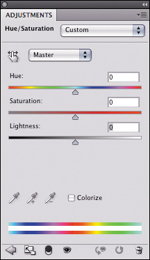
Figure 1.13.4. Setting the Saturation to −100%
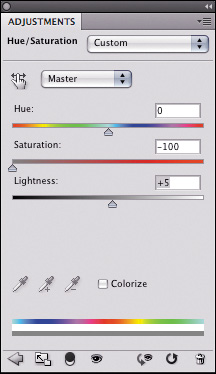
Figure 1.13.4. Gray image after the Hue/Saturation adjustment
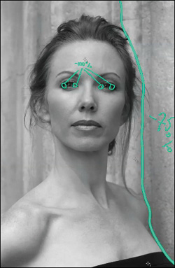
- Making sure that the layer mask is active, select the Brush tool (keyboard shortcut B). Expand the brush diameter to 600 pixels and set the opacity to 50%. Starting at the top of the image about halfway in, brush to the right, down the right side of the wall, making sure not to do any brushwork on Challen (Figure 1.13.5). Bring up the Fade effect dialog box, and move the slider right and left to see if you want more or less of the effect. I chose 38% (Figure 1.13.6).
Figures 1.13.5 and 1.13.6. Brushwork on right wall and then fading the effect with the Fade effect command

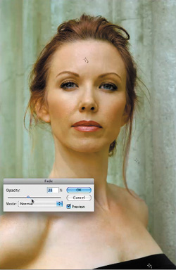
- Zoom into Challen’s face, around her eyes (Figure 1.13.7). Reduce the brush to 20 pixels and make sure that the brush opacity is set to 100%. Brush in all of the white in both of her eyes. You will notice that this is actually a bit too much, but I chose to do this because I wanted the desaturation to be greater in her eyes than in the wall. Also, I wanted to have some color bleed back into her image. One of the many advantages to using adjustment layers is that you can decrease opacity using the Opacity slider located at the top of the Layers panel. I chose 60% for this image. Examine the close-up of her eyes after the adjustment (Figure 1.13.8). Next, color back in the wall (Figure 1.13.9).
Figure 1.13.7. Zooming into Challen’s face
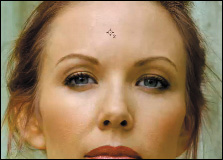
Figure 1.13.8. The eyes after the adjustment
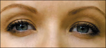
Figure 1.13.9. Brushing in the back wall
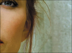
- Move the Hue and Saturation adjustment layer above the Midpoint Curves adjustment layer and turn the Midpoint Curves adjustment layer on.
The first part of the granular correction is done. You can see how an image-specific, dynamic workflow is developing. Throughout the course of this book, you should also be aware of how certain decision-making processes allow you to stay as close to the originally captured image data as possible, so as to minimize the cumulative aspects of artifacting, while allowing you to re-create your original vision.
Step 3: Merging Layers in “The Move”
You will now merge the copies of the layers that you have created thus far into a single new layer, while preserving the individual layers that you created earlier. Adobe Photoshop refers to this as Merge Stamp Visible. I prefer to refer to it as doing “The Move.” Note that you are merging the layers into one without flattening the image. This is an important distinction, because if you just merge layers, you also flatten the resultant image and lose all the original layers. This leaves you no exit strategy, and you will be unable to practice at practicing.
Make sure you are at the top of the layer heap by making the topmost visible layer active. Or, if you are working with a layer set, as you are in this image, make the layer set active. In this case, the layer set to make active is BP/WP/MP. For CS3 and above, press and hold Command + Option + Shift + E / Control + Alt + Shift + E. For CS2 and below, press Command + Option + Shift / Control + Alt + Shift, then type N, and then type E.
Note
Do not forget that when doing The Move, all layers that are turned on will be merged into one, both above and below the layer that is active. If after you do The Move, you notice that you have twice the effect that you had before you did it, you had adjustment layers turned on above the active layer or layer set. This is why you want the top layer, or top layer set, to be the active one.
You now have a base image layer on which you can start to work to make other aesthetically pleasing changes. Name it MASTER_1. Click Save As (Command + Shift + S / Control + Shift + S) and name the file SHIBUMI_16BIT. Save the image as a Photoshop document (.psd).
Note
I have a system for saving and naming files. I always save the layered files with which I am working as Photoshop documents (.psd). I save all of the files that I use for printing as Tiff files (.tif), but I do not save layered Tiffs. Not all programs that can open Tiffs can read layered Tiffs, and sometimes layered Tiffs can cause programs that cannot read them to crash. Also, the Windows operating system (OS) does not show thumbnails of either layered files or any file on the desktop, except for Genuine Fractal files (.stn). Because I will eventually scale all of my files, I save them as Genuine Fractal lossless files. Once they are scaled, I save the scaled file as a Genuine Fractal visually lossless file.
So that I can recognize how I saved a file, I add 16Bit or 8Bit to the filename. For Tiffs, I add the canvas size. For example, SHIBUMI_13×19.tif would mean that its canvas size is 13 by 19 inches. The reason that I use underscores instead of spaces is to guarantee that every OS can see and open the file. SHIBUMI.stn would mean that this is a saved Genuine Fractal lossless version of the file saved in its native resolution (the resolution in the original capture). SHIBUMI_24×30 _VL.stn would mean that the canvas is 24×30 inches and that it is a Genuine Fractal, visually lossless file that has been scaled to 24×30 inches. Genuine Fractals is the best way I know to scale an image, both up and down, and is a great way to losslessly compress an image so that it can travel with you. Always give your layers and files meaningful names, and always give yourself an exit strategy as you develop your personal approach to workflow.
If you are using a pen-based workflow with either a graphics tablet like the Wacom Intuos or pen display like the Wacom Cintiq, you can program any set of keystrokes into the pop-up menu, express keys, or Radial dial menu depending on which flavor of the device driver you are using. All you will have to do is click a button, and voilà — “The Move” will happen.
Creating the Illusion of DOF on Pixel Layers
In order to create the illusion of DOF, you are going to use three free third-party plug-ins, two from Nik Software (Skylight and Contrast Only) and one from onOne Software (FocalPoint 2.0).
The Skylight filter will be used to add warmth to the image by selectively brushing in those areas you want to appear to be in the foreground. (Warm colors create the illusion of moving the object forward in the composition.) Those areas that are not brushed in will appear to move backwards in the composition, because they will be cooler than those in the brushed-in areas. (Cool colors appear to recede.)
This goes back to creating a believable probability. In the real world, shadows tend to be bluer (cooler) than areas that are well lit. Areas that are lit tend to be red or yellow (warm). Generally, people tend to look better warmer than cooler. Thus, what you will do is create selective warmth in the image so that it follows the roadmap that you defined in your initial image maps. Now look at the L2D image map (Figure 1.14.1), the Lighting image map (Figure 1.14.2) and the Combined L2D and Lighting image maps (Figure 1.14.3).
Figure 1.14.1.
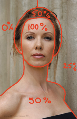
Figure 1.14.2.
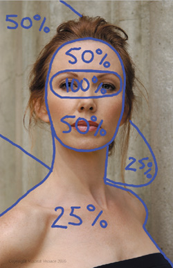
Figure 1.14.3.

Nik Software’s Contrast Only filter will be used to selectively add contrast to both aid in the replication of the way a lens would create DOF and to control how the viewer’s eyes moves through the image.
Before I talk about bokeh, you should know that when an optical lens is focused on an object, there is a direct relationship between the sharpness of the image and its contrast. Contrast is about “surface texture” while sharpness (resolving power) is about the distinctness of edges. As the surface textures of adjacent areas become more distinct, the boundary between them (the sharpness) increases.
A good lens will sharpen an image if certain characteristics are built into the glass, i.e., contrast and resolution capability. Some lenses are better than others because of these characteristics. In optics, as sharpness and contrast decrease, blur increases. When purchasing a lens, its ability to go from sharpness (focus) to blur (out-of-focus) is an often overlooked quality. This quality is called bokeh (pronounced BO-KAY). The term comes from the Japanese word, boke (pronounced BO–KA), which means blur, and aji (pronounced AE), which means quality.
In photography, bokeh is the aesthetic quality of the blur in out-of-focus areas of an image, or the way the lens renders out-of-focus points of light. When deciding what lens to buy or use, strongly consider one that exhibits excellent, aesthetic bokeh. Much has been written about bokeh, and I encourage you to read more about this concept.
What you will do in the next series of steps is to create three layers, which, when combined, will replicate a lovely and subtle bokeh. In the image of Challen, I wanted to create the illusion that she is farther away from the wall than she actually was. I am going to have you do this by, first, warming up the image, then by building up the image’s contrast, and, finally, by introducing blur.
Step 1: Getting the Red In: Correcting for the Blue Color Cast with Nik’s Skylight Filter
Up to this point, you have used adjustment layers, which are simply layers of math over your image, and have not actually altered the pixels. This is about to change. Previously, you created your first layer, MASTER_1, which was the culmination of all of the work you did on the Black, White, and Midpoint Hue/Saturation adjustment layers.
Whenever possible, I try to come up with a “Photoshop” way of doing things, and I am successful most of the time. But what makes Photoshop such a unique software package is that Adobe designed a way for us to use add-ons (called plug-ins) without affecting the core of the program. In my pursuit of a smoother workflow, I have become an advocate of the filters made by Nik Software.
Note
If you have not already downloaded the free versions of the Nik Software Skylight, Tonal Contrast, and Contrast Only filters, you can find them at www.welcome2oz.com. You will need to install these plug-ins for this next part of the lesson.
A Skylight filter can correct for the fact that shade and shadow light tends to be bluer than direct light, and direct light tends to be bluer than early morning and late afternoon light. The filter scans the image and determines how much, and where, red needs to be added to counteract any blue cast.
- Duplicate the MASTER_1 layer (Command + J / Control + J).
- Go to Filter > Convert for Smart Filters (Photoshop will make the layer you just duplicated into a Smart Filter) (Figure 1.15.1).
Figure 1.15.1.
- Duplicate the MASTER_1 copy layer twice (Command + J / Control + J). You should now have three Smart Filter layers.
Note
A quick way to duplicate a layer is to use Command + J / Control + J. Although this is the command for duplicating a selection, you can also use it to duplicate a layer.
Now that you have created your first Smart Layer, or Smart Filter, you may have been surprised at how quick and easy it was. Smart Filters take a while to make, but not to duplicate. If I know that I am going to use different effects or multiple filters, but I do not want to work on just one layer or on the same master layer, I will make several duplicates and throw away the ones I do not need when I am finished.
If you use CS3 or above, you should use Smart Filters (if you do not already) because they contribute to creating a non-destructive workflow, and because you can undo whatever you may have done. Even after you have made a print, all you have to do is go back to that Smart Layer and adjust it if you want to sharpen differently, change the lighting effects, or the color. The only down side it that Smart Filters make the file bigger. Regardless, I believe that Smart Filters and Smart Objects are the future of image editing.
- Make the layer MASTER_1 copy three, the active layer, and rename it SKYLIGHT.
- Choose Filter > Nik Software > Color Efex Pro 3.0: Versace Edition > Skylight Filter. When the dialog box comes up, select Skylight (Figure 1.15.2). Zoom out to see the full image. Leave the default at 25%, which is usually the correct amount, and click OK. Compare the before (Figure 1.15.3) and after (Figure 1.15.4).
Figure 1.15.2. Applying the Skylight filter
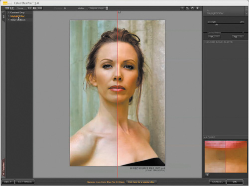
Figure 1.15.3. Before the Skylight filter
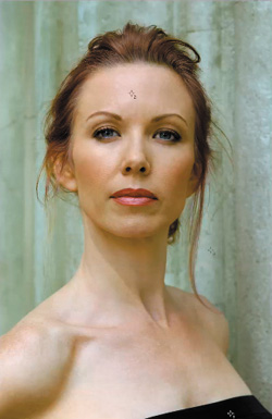
Figure 1.15.4. After the Skylight filter
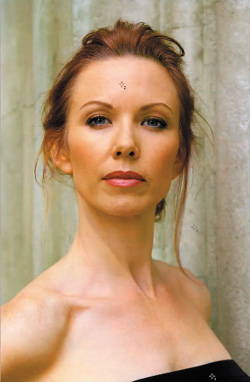
You should see that the blue cast has been removed from this entire image so that it appears warm, which is wonderful for Challen’s face, but not for her body, and definitely not for the background. You want the background to appear to be in shadow, which requires a blue cast. In addition to trying to create DOF, you are also trying to create an image that appears to have been lit with “hot” or tungsten lights. In order to create this believable probability, you must pay attention to the areas that must be lightened. As you go about the business of building this image, each step must build upon the last in a way that minimizes artifacts.
- Create a layer mask on the SKYLIGHT layer and fill it with black.
Note
You are filling the layer mask with black, because you want to conceal more than you want to reveal (see 80/20 rule sidebar.)
To create a layer mask, go to the bottom of the Layers panel. Holding down the Alt / Option key, click on the Add Layer Mask button (the third from the left). This is the one-click way to create a layer mask and fill it with black.
- Make the L2D IM and LIGHTING IM layers visible so that you can analyze how to selectively warm this image (Figure 1.15.5).
Figure 1.15.5. The combined image maps
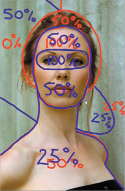
For a moment, review your lighting decisions. The model’s eye should be the most brightly lit, less on her face, then her hair, and the area on the wall should receive the least light.
Take a moment to conceptualize this task. Because you are working with a layer mask filled with black, but you are painting with white, you are dealing with a negative image as you would in a black-and-white darkroom. Therefore, you are working in reverse.
You are aiming to build up different levels of warmth (the warmth that you just created using the Skylight filter), and since you want the eyes to be brightest, start by brushing that area. (Remember, all brushwork is cumulative.)
- Choose a very soft brush, roughly the size of the eye socket (400 pixels), but big enough to sweep across her eyes. (That is where the key light is going to go.) Start with an opacity of 50% (keyboard shortcut 5), and brush across her eyes.
- Bring up the Fade effect dialog box (Command + Shift + F / Control + Shift + F). This is the area to get the greatest Skylight filter effect, so move the slider to the right until you reach 61%, the value I chose. Click OK (Figure 1.15.6).
Figure 1.15.6. Set the Amount to 61%
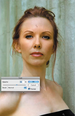
- Increase the brush size (the right bracket key) to 700 pixels, and, following your image map, brush in her face and hair.
- Bring up the Fade effect dialog box (Command + Shift + F / Control + Shift + F) and move the slider to the right to 65%. Click OK. Compare the before (Figure 1.15.7) and after (Figure 1.15.8).
Figure 1.15.7. Before the brushwork and Fade effect

Figure 1.15.8. After the brushwork and Fade effect
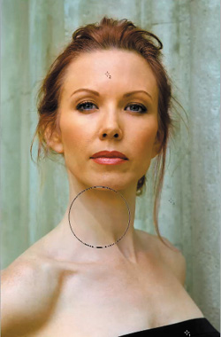
- Bring up the Fade effect dialog box (Command + Shift + F / Control + Shift + F), move the slider to the left, and lower it to an opacity of 34% (Figure 1.15.9). Paint in a small area of her body and examine the effect (Figure 1.15.10).
Figure 1.15.9. Setting the Fade effect to 34%
Figure 1.15.10. Brushing in the effect on her body
The last thing to do is to brush in the area where you will place your background light.
- Following the image map and using a 700 pixel diameter soft brush, brush on a diagonal from the upper left corner of the whole image to the area just above Challen’s shoulder and neck. Leaving that area at 50% opacity, brush in the area just above her right shoulder, bring up the Fade effect dialog box (Command + Shift + F / Control + Shift + F) and move the slider leftward to an opacity of 34%. Compare the image before adding the layer mask (Figure 1.15.11) and after the layer mask (Figure 1.15.12).
Figure 1.15.11. The Skylight filter before the layer mask

Figure 1.15.12. The Skylight filter applied selectively with the layer mask
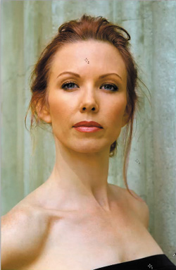
Note
There are several areas of gaps and overlap in the layer mask. Using the technique that you learned in the previous section, tighten them up.
Step 2: Creating Selective Contrast with Nik Software’s Contrast Only Plug-In to Replicate Realistic Lens Bokeh
When referring to how optical lenses record images, it can be said that contrast and blur are directly related. This may not be true when you create blur in a image using image editing software. Computer manipulation allows you to apply both contrast and blur to your image file, so they are not interdependent as they are if the blur was created by a lens. Although you can increase contrast with the brightness and contrast filters in Photoshop—or even better, with a Curves adjustment layer—Nik Software’s Contrast Only plug-in does a better job than either of these and, not only offers significantly greater control, it comes free with this book.
- Go to Filter > Nik Software > Color Efex Pro 3.0 Versace Edition (Figure 1.16.1). When the Plug-in dialog box comes up, select Contrast Only.
Figure 1.16.1. Opening Color Efex Pro 3.0
Begin by adjusting the contrast of Challen’s face. Because the contrast of her face is the critical part of this image, you should bias your aesthetic decisions in that direction.
- Click on the Contrast slider. (The default is 50%.) Move the slider to the right to increase the contrast. Move it to 64%, which is too much, and then come back to 55%, a reasonable setting (Figure 1.16.2).
Figure 1.16.2. Moving the Contrast slider to 55%
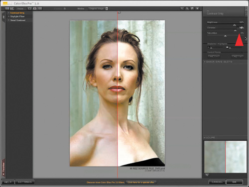
- Click on the Brightness slider. Move the slider to the left to diminish the brightness. (The default is 50%.) Move the slider to 35%, which is too much, and then retreat to 41%, a usable position (Figure 1.16.3).
Figure 1.16.3. Moving the Brightness slider to 41%
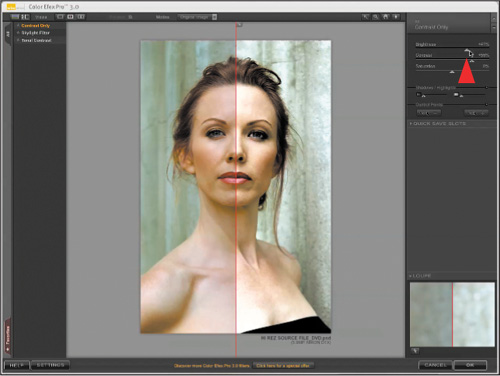
You have completed a global adjustment of the contrast and brightness. Although there are still some blocked shadows and overly bright highlights, you will address them in a moment. A bigger issue, however, is that when you compare the before and after aspects of the image in the Contrast Only dialog box, you now have some issues with image saturation. Specifically, you lost some of it and will have to correct that.
Thus far, the adjustments you have made to brightness and contrast could have been done in Photoshop, but the following steps will more elegantly and easily be done using Nik’s Contrast Only filter.
- Click on the Saturation slider, and move it to the right, until you match the saturation to the before side of the image in the preview area of the plug-in dialog box, which for this image occurs at 16% (Figure 1.16.4).
Figure 1.16.4. Moving the Saturation slider to 16%
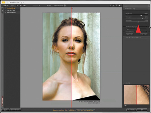
It is time for you to address the more granular issues that were produced after you introduced contrast into this image: blocked up shadows and loss of image detail. The method that I will have you use to correct these problems (the Protect Shadows and Protect Highlights sliders in the Contrast Only plug-in) allows you to control how much of the shadows and highlights you affect (see the Protect Shadows and Protect Highlights sidebar for how this works.)
- Click on the Protect Shadows slider and move it to the right until the shadow is no longer blocked up. Compare the before (Figure 1.16.5) and after (Figure 1.16.6).
Figure 1.16.5. Before using the Protect Shadows slider

Figure 1.16.6. After using the Protect Shadows slider
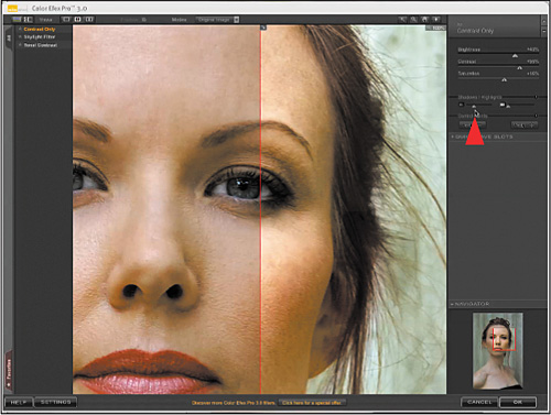
The Protect Shadows and Protect Highlights sliders help you protect image details at both ends of the tonal range (from pure white with no texture to pure black with no detail) (Figure 1.16.7). The controls take advantage of the TrueLight™ function in Color Efex Pro 3.0. and appear on the Advanced tab in Color Efex Pro 2.0. When collapsed, this section displays one slider for protecting shadows and one for protecting highlights. As you click and drag either slider to the right or left to increase or decrease protection, notice the change in the details in the image. When expanded, this section displays not only the sliders, but also a histogram representing the full tonal range of the active image after the current enhancement has been applied. The histogram changes in real time as you adjust the filter controls and Protect Shadows/Protect Highlights sliders. The colored areas at both ends of the histogram help identify potential problems. The top and bottom 2.5% of tonal values (representing Shadows without Detail on the left and Highlights without Detail on the right) appear in red. The next 2.5% of the shadows and highlights (indicating Shadows with Detail on the left and Highlights with Detail on the right) appear in green. Connected to each of the four colored areas (Shadows without Detail, Shadows with Detail, Highlights without Detail, Highlights with Detail) are numerical call-outs displaying the percentage of pixels from the active image in each of those four areas after the enhancement has been applied.
Figure 1.16.7. The Protect Shadows and Highlights sliders
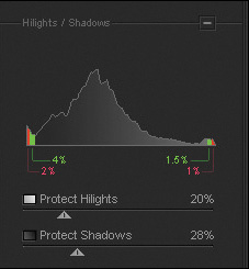
The Protect Shadows and Protect Highlights sliders help you keep your image details from falling into these areas. For best results, keep the greater part of the image between the green areas (Shadows with Detail and Highlights with Detail) of the histogram. Portions of the image in Shadows without Detail will likely print pure black; those in Highlights without Detail will likely print as paper white. Click and drag the Protect Shadows slider to the right to adjust the filter’s effect and prevent details from being moved into the Shadows without Detail area. Click and drag the Protect Highlights slider to the right to adjust the filter’s effect and prevent details from being “blown out” or being moved into the Highlights without Detail area.
I am going to introduce you to one of the most powerful functions of the Contrast Only plug-in: Control Points. (See sidebar for detailed information.) Control Points allow you to create an effect in an isolated object within a photograph. After you place a Control Point, the software analyzes its color, tonality, detail, and location, and applies the desired effect. There are two types of Control Points: Additive and Subtractive.
- Click on the Additive Control Point (Figure 1.16.8), and place it on the middle of Challen’s forehead by clicking on that area (Figure 1.16.9).
Figure 1.16.8. The Additive Control Point button
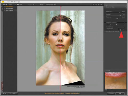
Figure 1.16.9. Placing an Additive Control Point on her forehead
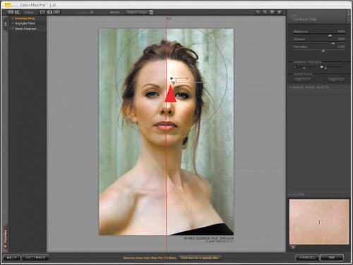
Once you have initially placed your Control Point, you can fine tune its effect by moving it. When you move a Control Point, it will update in real time. You can also control the size of the area that you want the Control Point to influence.
- Click on the Control Point and drag it to the area between her eyes at the top of the bridge of her nose (Figure 1.16.10).
Figure 1.16.10. Moving the Control Point between her eyes
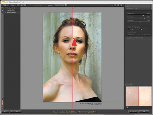
A Control Point automatically isolates objects based on their unique characteristics and permits you to easily apply enhancements using sliders. This is done with simple click and drag functionality, so there is no need to create complex selections, masks, or layers found in most conventional editing tools. Rather, changes can be made using a single, easy-to-use method that greatly expands your image editing capabilities. Using U Point® powered Control Points, you simply start by identifying an object, area, or region in a photo that you wish to enhance, and then you drag and drop a Control Point onto the image.
Once a Control Point is placed, the Control Point automatically:
- reads RGB and location values for each Control Point that is placed on the image.
- calculates additional values of hue, saturation, brightness (lightness), and image detail to create a complete and unique set of U Point Pixel Characteristics.
- incorporates the U Point Pixel Characteristics into a central, intelligent, blending function. U Point technology’s central blending function enables you to adjust the entire range of parameters that control color and light (including, Red, Green, Blue, hue, saturation, brightness, contrast, and warmth, as well as the size of the area to be controlled) using a set of sliders associated with each Control Point.
When an additional Control Point is placed on the image, U Point Pixel Characteristics for that specific Control Point are calculated and are then factored into the central blending function. As more Control Points are placed on the image, the central blending function becomes more intelligent, enabling you to make even more refined and precise changes in the image. You control color, light, contrast, and tonality.
The Control Points are interdependent and communicate to combine and blend enhancements naturally. They can be easily adjusted or undone at any time, regardless of the order in which the change was made or the sequence in which the points were placed (Fig.1.16.11).
Figure 1.16.11.
You can either increase or decrease the amount of the effect with the Opacity handle, the bottom one, or you can increase or decrease the size of the area that will be affected with the Radius handle, the top one.
- Click on the Radius handle and move it inward so that the outer edge of the circle is touching her hair. Then, further fine tune the effect by moving the Control Point to the red dividing line that runs down the center of the image.
- Click on the Subtractive Control Point (Figure 1.16.12) and drag it to upper right corner of the wall that is in the background (Figure 1.16.13). Click on the Radius handle and extend it to 67%.
Figure 1.16.12. The Subtractive Control Point button
Figure 1.16.13. Placing a Subtractive Control Point on the wall
- Create a second Subtractive Control Point, and move it to the lower right of the wall above Challen’s shoulder. Adjust it to the same radius as the first Subtractive Control Point that you placed (Figure 1.16.14).
Figure 1.16.14. Placing a second Subtractive Control Point
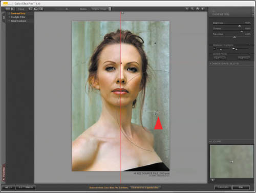
- Create a third Subtractive Control Point and move it to the lower left of the wall above Challen’s shoulder. Adjust it to the same radius as the first Subtractive Control Point that you placed (Figure 1.16.15).
Figure 1.16.15. Placing a third Subtractive Control Point on the wall to the left of Challen
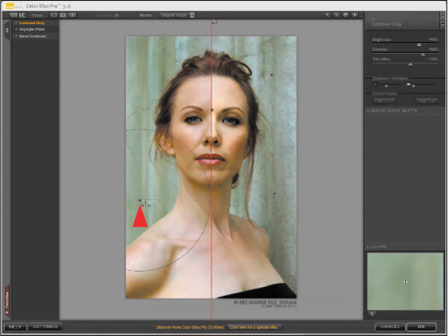
- Create a fourth Subtractive Control Point and move it to the upper left of the wall next to Challen’s head. Adjust it to the same radius as the first Subtractive Control Point that you placed (Figure 1.16.16).
Figure 1.16.16. Placing a fourth Subtractive Control Point on the upper left wall
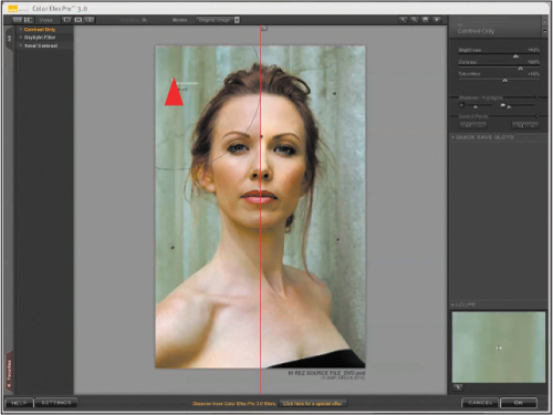
The result of using Additive and Subtractive Control Points is that the background has no contrast, but the model’s face does.
- If you would like to increase the contrast, move the Contrast slider to 73%.
- Click OK.
Compare the image before the Contrast Only filter (Figure 1.16.17) and after the Contrast Only filter (Figure 1.16.18).
Figure 1.16.17. Before the Contrast Only filter
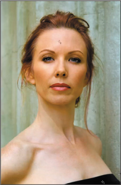
Figure 1.16.18. After the Contrast Only filter
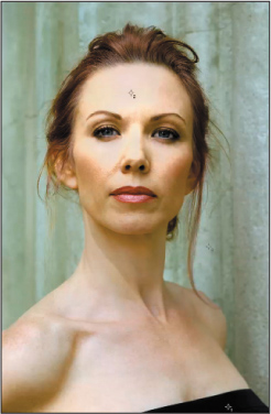
- Duplicate the SKYLIGHT layer mask and drag it down to the CONTRAST layer mask. You do that by holding down the Option / Alt key, clicking on the SKYLIGHT layer mask, and dragging it down to the Contrast layer. Once finished, you should see in the Layers panel that the Contrast and Skylight layers have the same layer mask (Figure 1.16.19). The image now looks like it does in Figure 1.16.20.
Figure 1.16.19.
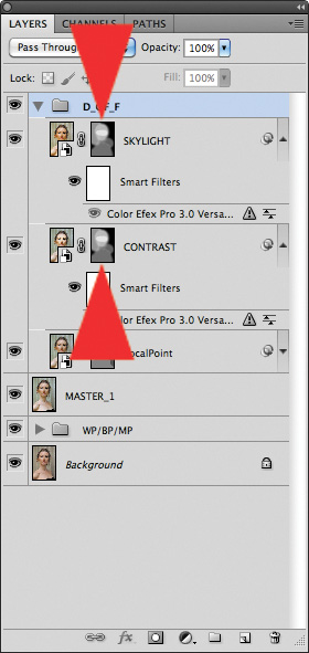
Figure 1.16.20. The image after duplicating the layer mask
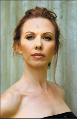
You now have some options to consider. You could move the Contrast layer above the Skylight layer, or you could leave it where it is beneath the Skylight layer. For this image, I prefer to have the Skylight layer on top and the Contrast layer just beneath it.
Another option is to lower the amount of the Skylight or Contrast layer to further dial in the effect. For this image, I chose to reduce the Skylight layer to an opacity of 70% (Figures 1.16.21).
Figure 1.16.21. The image after reducing the Skylight layer opacity to 70%
You should notice that the model’s image is beginning to appear forward from its real position. Once you introduce blur, you will have completed the illusion of DOF.
Step 3: Creating Selective DOF Using onOne Software’s FocalPoint 2.0 to Replicate Realistic Lens Bokeh and DOF
The definition of a Circle of Confusion: A bunch of photographers sitting around a table trying to explain Depth of Field.
—Michael Reichmann
As I briefly discussed earlier in this chapter, computer manipulation allows you to apply both contrast and blur to your image file, so they are not interdependent as they would be if the blur was created by a lens. This distinction is important because in a digital image file you can apply blur without diminishing contrast.
The model’s image is beginning to appear forward from its real position because you have introduced selective warmth, using the Nik Software Skylight and Contrast Only filters on her face and torso, while leaving the background unaffected. Because your aim is to create a probable believability, while keeping your workflow dynamic and non-destructive, you want the viewer’s eye to move through your image so that they are unaware of the journey. This will happen once you introduce realistic, selective blur, the focus of the next step.
Plumbing the Depths of DOF
DOF generally refers to the area that is in focus both in front and behind the true plane of focus. Actually, it is best conceptualized as the area of acceptable out-of-focus outside of the plane of focus. DOF varies depending on camera type, recording media (film or digital), aperture, and focusing distance. Even print size and viewing distance influences our perception of DOF.
When you consider DOF, there is no abrupt change from the area of sharp focus to areas of un-sharp focus; the change is a gradual one. One of the many common misconceptions about DOF is that its area encompasses everything that is in focus. Not true. According to optical physics, there is only one plane that is in focus in a photograph, that plane on which the lens is physically focused (the plane of critical focus). Everything else is less sharp; our eyes may simply not perceive it.
What we perceive to be in focus has a lot to do with the resolving characteristics of lenses, film, and silver-based photographic papers. A good or great lens can resolve an image of 200 line pairs (LP), or 200 pairs of black and white lines per centimeter. Black and white silver-based films can resolve approximately 175 LP, color film approximately 150, and photographic papers between 50 and 75. In other words, the final resolution is no better than the paper’s ability to record it. Fortunately, the human eye will not detect blur until the resolution falls below 50 to 75 LP, so even though anything that was captured and recorded above 75 LP is lost in the printing process, we remain blissfully unaware of it.
Digital photography and inkjet printing has changed all of this. Lenses and sensors both resolve 200 LP, and consumer inkjet printers can print 150 LP—twice to three times the resolution of silver-based papers. Additionally, professional inkjet printers can resolve upwards of 300 LP—even more than lenses, CCDs, and CMOS sensors can resolve. What this means is that if you want three elements in an image to be in focus, rather than stopping the lens down in traditional wet photography methods, in digital, you will need to take three separate images of the three elements you want in focus to ensure that you get the detail you want in each. (You will explore this further in Chapter Three of this book.)
In any image, there is much more blur than there is focus. And blur is not simply a measurement of what is not in focus. Blur has a quality, a bokeh. This is an important aesthetic element and should be considered in every image. (More in a moment.)
Because the point at which focus transitions to out-of-focus is a difficult one to perceive, the term “circle of confusion” is used to define how much a point needs to be blurred in order to be perceived as not sharp. As well stated in Sean McHugh’s discussion of DOF (http://www.cambridgeincolour.com), “When the circle of confusion becomes perceptible to our eyes, this region is said to be outside the DOF and thus no longer acceptably sharp.”
What Is a Circle of Confusion?
The Glossary of Digital Photography (John Blair, Rocky Nook Inc., 2008) defines a circle of confusion this way: “When a lens is operating properly, subjects that are perfectly in focus should come to a point at the plane of the sensor. This is known as the focal point of the lens. Subjects closer or farther away will not be in as good of focus as the main subject. Instead of coming to a point at the sensor, the subjects create a small circle or other shape depending on the lens and aperture configuration. If the circle is sufficiently small, the subject is considered to be in focus. As the circle grows larger, due to subject distance from the lens, it becomes more noticeable. This circle is known as a circle of confusion. The range of distances of the subject from the lens when the circle is small enough not to be noticeable is known as the DOF. The largest circle of confusion still considered acceptably small, such that the subject is in focus, is known as the maximum permissible circle of confusion.” (Real lenses do not focus all rays perfectly, so that a point is imaged as a spot rather than a point. The smallest such spot that a lens can produce is often referred to as the circle of least confusion.)
In the description above, note the relationship of DOF and the circle of confusion (COC). In photography, a rudimentary understanding of COC is essential to your understanding of DOF.
As I discussed earlier in the Depth of Field sidebar, “It has been shown that if the depth of the area that appears to be in focus in front of the true plane of focus is one foot, then the area that appears to be in focus behind the true plane of focus is two feet. This works out to a ratio of one-third in front in focus to two-thirds behind, i.e., twice as much behind will be in focus as in front.”
The distance that appears to be in focus depends on two factors: the size of the lens aperture and the distance from the camera to the subject. The larger the aperture, the shallower the area that appears to be in focus; the smaller the aperture, the greater the area that appears to be in focus. Additionally, the farther away a subject is from the camera, the greater the DOF, i.e., the more that will appear to be in focus. Conversely, the closer the subject is to the camera, the shallower the DOF, i.e., the less that will appear to be in focus.
What No Focal Length?
Many photographers have the mistaken belief that shorter focal length lenses have a greater DOF than longer focal length lenses. Telephoto lenses appear to have a much shallower DOF, because they are most often used to make the subject appear larger when you cannot get physically as close to the subject as you might like. Sean McHugh of Cambridge Colour states, “If the subject occupies the same fraction of the view-finder (constant magnification) for both a telephoto and a wide angle lens, the total DOF is virtually constant with focal length!” This means that it is the angle of view, and not the focal length, that determines DOF. I will illustrate why this misunderstanding exists with the following example. If I set up a tripod and shoot a scene using a 200mm lens, and then change to a 35mm lens at the same position without changing the aperture, the 35mm frame will appear to have a greater DOF. This occurs, however, only because the 35mm lens has a much larger field of view. To accurately compare the DOF of the 200mm lens to the 35mm lens, I must move in with the 35mm lens until the field of view exactly matches the field of view I had with the 200mm lens at the original position. When the resulting images are compared, the DOF for the two lenses will be exactly the same.
Compare the DOF images that were shot with a 35mm lens, a 70mm lens and a 135mm lens of the Golden Gate Bridge. (Figures 1.17.1, 1.17.2, and 1.17.3)
Figure 1.17.1. Shot with a 35mm lens
Figure 1.17.2. Shot with a 70mm lens
Figure 1.17.3. Shot with a 135mm lens
Note
Some of the best examples of this concept can be found in Michael Reichmann’s landscape article, “Do Wide Angle Lenses Really Have Greater Depth of Field Than Telephotos?” (http://www.luminous-landscape.com/tutorials/dof2.shtml). See also Sean McHugh’s discussion of DOF (http://www.cambridgeincolour.com/tutorials/depth-of-field.htm).
The Bouquet of Bokeh
For me, DOF is more about the quality of the blur, the bokeh, than it is about what is actually in focus. This is because everything that is not in the plane of focus is at varying levels of acceptable out-of-focus. Thus, most of your image is affected by bokeh. Bokeh is an immeasurable quality. It describes the feel of the blur, its smoothness. It is inherent in how an optical system bends the light and handles those rays of light that are not in focus and which blurs the object’s edges in an aesthetically, visually, appealing way. Good bokeh consists of a gentle smoothness where the blur gradually occurs in a subtle way.
Effing the Ineffable
Good bokeh is not necessarily inherent in lens design, but different lenses produce different bokehs. A lens is defined simply as “a transparent optical device used to converge or diverge transmitted light and to form images.” The image resulting from an excellent lens will be one where the edges of objects are extremely well-defined with little gradual blur. A technically perfect lens, however, does not necessarily produce a good bokeh. In fact, that technically perfect lens might render out-of-focus points of light with sharply defined edges rather than with the smoothness that you may find more visually appealing and desirable. It is the imperfections, the peccadilloes of design, that give a lens uniqueness. The finished image often owes its beauty to these imperfections.
Bokeh can be compared to the crazing on an old piece of porcelain that has hundreds of random, minute cracks that occur over time due to an imperfect glazing process and thermal stresses. The result is a vase or cup that is beautiful because of its imperfections. Although you may know what causes these imperfections, there are no measurements or rules that allow you to control it. It occurs in a random and beautiful way.
No one knows why one lens design produces better bokeh than another. What matters is that you are aware that this phenomenon occurs, and that you should pay attention to its presence or absence when choosing your glass. Among the things that affect lens bokeh are: the number of blades in the aperture diaphragm; the shape of the diaphragm opening; the number, configuration, and grouping of lens elements; the length of the lens barrel; the types of lens aberrations; the coatings on and the type of glass used in the lens, the speed of the lens; and more. This is why the same image shot with a 24–70mm zoom, a 24–120mm zoom, and a 70–200mm zoom lens, all at a focal length of 70mm, would look different. It is up to the photographer to test his or her lenses and decide which ones impart the illusive quality that he or she seeks to any particular subject matter. See Figures 1.17.4, 1.17.5, and 1.17.6.
Figure 1.17.4. 24–70mm lens
Figure 1.17.5. 24–120mm lens
Figure 1.17.6. 70–200mm lens
I am having you consider bokeh in this lesson, because you are trying to replicate the reality of a shallower DOF than you have, so that Challen appears to be standing farther away from the background than she actually was. If you understand that a lens is more about blur than focus, and that the blur that you are trying replicate has a unique quality that is lens specific, then this understanding will help you decide how to best create the believable probability that this image was shot at a shallower DOF than it really was.
Note
Two very good explanations and discussions of bokeh are Harold Merklinger’s at http://www.luminous-landscape.com/essays/Bokeh.shtml and Ken Rockwell’s at http://www.kenrockwell.com/tech/bokeh.htm
Figure 1.17.7. Good bokeh: The blur is completely undefined.
Figure 1.17.8. Neutral bokeh: The blur circle is even and its edges retain definition even though the light circle is blurred. (This is the way most modern lenses are designed.)
Figure 1.17.9. Bad bokeh: The blur circle’s edge is overly defined and there is a ring around the center that is darker than the center.
Focusing in on FocalPoint 2.0
To my knowledge, there is no better way to create realistic lens blur, and either enhance the existing bokeh of a lens or replicate lens bokeh, than by using the FocalPoint 2.0 plug-in.
First, there are two parts to the user interface (UI): FocusBug (Figure 1.18.1) and its slider controls (Figure 1.18.2). You will probably need only the FocusBug, but the sliders provide fine tuning should you need it.
Figure 1.18.1. The FocalPoint UI
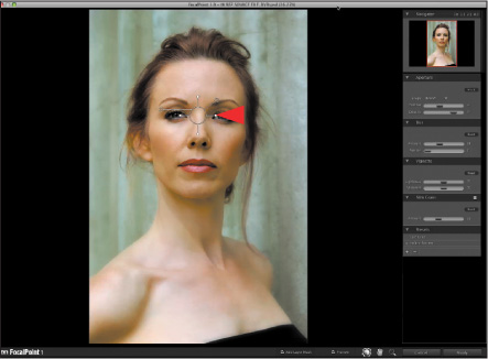
Figure 1.18.2.
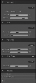
Take a look at the Panels side of the UI.
1. Navigator Panel: displays an overview of the entire image along with a red box marking the area displayed in the preview area (Figure 1.18.3).
Figure 1.18.3.
2. Aperture Panel: contains controls for type of aperture, round or planar, as well as its feather and opacity functions (Figure 1.18.4).
Figure 1.18.4.
The Aperture Panel lies just below the Navigator and contains controls for aperture shape as well as its feather and opacity functions. Feather and opacity can also be adjusted with the FocusBug.
Aperture Shape
This pop-up allows you to control the shape of the sweet-spot. You can select between round (default) or planar. The FocusBug tool changes appearance from a round body (the default creates a round or oblong sweet-spot) to a square body. The round body is similar to using a selective focus lens and its blur extends to all sides of the image. (The sweet-spot is the area that is not affected by blur and is in focus.)
The second shape, planar, simulates a tilt-shift or view camera appearance. It creates a sweet-spot that slices through the image from one side to another.
Feather
Feather controls how hard the edge of the sweet-spot will be. The harder the edge, the more obvious the transition will be between the sweet-spot and the blur. Generally, a setting of 25–50 is used. Feather also controls the angle of the right antenna.
Opacity
This controls the sweet-spot’s opacity. At 100%, the sweet-spot is completely protected from blur. As the opacity is decreased, the sweet-spot begins to blur. In most cases, you will want the opacity to remain at 100%. The opacity is also controlled with the left antenna.
3. Blur Panel: contains controls for the amount and type of blur, both of which can be adjusted with the FocusBug (Figure 1.18.5).
Figure 1.18.5. Blur panel
Amount
This slider controls the amount of blur, and is typically set between 25–75%. The amount can also be controlled with the right antenna.
Motion
The Motion slider controls the amount of motion or distortion in the blur. At the minimum setting, the blur appears uniform. As you increase the angle (amount), the blur will appear to have more motion. This simulates the edge of an image circle where the blur becomes more distorted and is useful for a more dramatic look or simulating the bokeh of certain lenses.
4. Vignette Panel: contains controls for the amount and brightness, as well as the midpoint of the vignette (Figure 1.18.6).
Figure 1.18.6. Vignette panel
The Vignette panel is located under the Blur panel and contains the controls for adding realistic vignettes to an image. Adding a vignette is a classic method for focusing the viewer’s eye on the subject. The shape of the vignette is always round and will follow the sweet-spot.
Lightness
The Lightness slider controls the amount and brightness of the vignette. At the neutral position (in the slider’s middle), there is no vignette. Moving the slider to the right yields a dark vignette, while moving it to the right yields a light one.
Midpoint
The Midpoint slider controls the relative size of the vignette in relation to the sweet-spot. Low values add a large vignette that is tight around the sweet-spot, while large values add a smaller vignette that affects only the image’s edge.
5. Presets Panel: lists the categories and presets and allows for their creation and loading (Figure 1.18.7).
Figure 1.18.7. Presets panel
6. FocusBug: The main control for FocalPoint 2.0, the FocusBug controls the size, position, and shape of the sweet-spot. Its antennae adjust the controls for the Aperture and Blur panels as well (Figure 1.18.8).
Figure 1.18.8. FocusBug
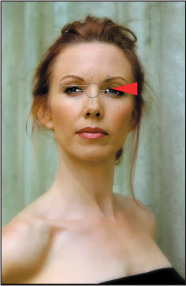
7. Guide Grid: The guide grid shows the size and shape of the sweet-spot and can be used to control its 3D tilt (Figure 1.18.9).
Figure 1.18.9. Guide grid
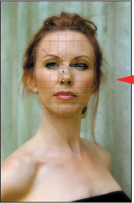
8. Toolbar: contains the Zoom and Pan tool for navigating the image. It also contains the FocusBug tool for adjusting the FocusBug and contains the preview on/off toggle (Figure 1.18.10).
Figure 1.18.10. Toolbar
![]()
9. Masking Options: adds a layer mask to the results in Photoshop allowing the selective application of effects.
10. Film Grain Panel: controls the addition of simulated film grain (Figure 1.18.11).
Figure 1.18.11. Film Grain panel
The Film Grain panel is located under the Vignette panel and contains the controls for adding film grain, or noise to the blur. Adding film grain can replace grain lost during the blurring process so that a realistic image is maintained. It is also useful to prevent posterization during printing. To toggle the Film Grain effect on and off, use the toggle on the right side of the panel title bar.
Amount
The Amount slider controls the amount, or opacity, of the film grain. It is a good idea to zoom into 1:1 (100%) when adjusting the amount.
Getting Buggy: Using the FocusBug
The FocusBug is the main control for using FocalPoint 2.0. It appears as a wireframe representation of an insect with a body, legs, and antennae. The FocusBug controls many features of the sweet-spot: its position; size; shape; the amount and type of blur; its feather and opacity.
FocusBug Shapes
Already discussed, the FocusBug has two shapes, round (default) and planar, and is controlled in the aperture panel from the shape pop-up.
Adjusting Size, Shape, and Position
The FocusBug controls the position, size, and shape of the sweet-spot. To position the FocusBug, make sure you have it selected from the toolbar. Then click inside the body of the bug, hold, and drag it into the middle of the area that you want to keep in focus (the sweet-spot). In order to control the size and shape of the sweet-spot, you will need to manipulate the FocusBug’s legs, the shorter appendages that extend out of the FocusBug body. On the round FocusBug there will be four legs; on the planar, only two. To adjust a leg, click, hold, and drag it with your mouse. If the end of a leg glows blue when your mouse pointer approaches it, you can select it. The length of the legs control the size and shape of the sweet-spot. You can also rotate the legs around the body to change the angle of rotation of the sweet-spot (Figure 1.18.12).
Figure 1.18.12. FocusBug diagram
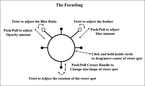
Note
It is often useful to turn on the grid when adjusting the FocusBug. This will allow you to see the exact size, shape, and position of the sweet-spot. You can turn on the grid by going to View > FocusBug Grid and selecting Auto or On.
Using the Antennae
The antennae of the FocusBug control the amount and type of blur as well as the feather and opacity of the sweet-spot. You adjust the antennae as you did the legs. Click, hold, and drag the antenna you wish to adjust. The right antenna controls the amount and type of blur. The longer the antenna, the more blur you will get. The angle of the antenna in relation to the body controls the feather or the transition between the sweet-spot and the blur. It is best to set the amount to 100% by pulling the right antenna to its longest position and then adjusting the feather at this setting. This will make the feather more obvious while you adjust it. Once the feather is set you may readjust the amount.
Note
Locking the antenna allows adjustment of only one variable at a time. By holding down the Shift key while adjusting an antenna, it will be locked to adjust only the antenna length. You may hold down Shift + Command / Shift + Control to adjust the angle instead.
The left antenna controls the type, or mix of blurs, as well as the opacity of the sweet-spot. The angle of the left antenna controls the type or mix of blurs. This is analogous to the Motion slider in the Blur panel. At the minimum setting, the blur will appear to be uniform. As you increase the angle (amount), the blur will appear to have more motion, which is useful when you want a more dramatic look or are trying to simulate certain lenses. The length (of the left antenna) controls the opacity of the sweet-spot, which in most cases you will want to set to 100%. This protects the sweet-spot from any blur.
Adjusting 3D Tilt
You can also use the FocusBug to tilt the plane of focus just like using a view camera. This will vary the blur on each side of the sweet-spot. To control the tilt, click and hold the Option / Alt key, and then click and drag inside the body of the FocusBug. A grid will appear, and as you move your cursor inside the FocusBug’s body, the grid will tilt in three dimensions. You can reset the tilt by holding Option / Alt and double-clicking inside the FocusBug’s body.
Note
Unlike a tilt-shift lens or view camera movements, FocalPoint 2.0 can only reduce the amount of sharpness, not improve it.
Mask View
Using Mask View will enable a black and white mask view of the sweet-spot. This can help you to see the bounds of the sweet-spot as well as understand the effects of the 3D tilt. To enable the Mask View, go to the View menu and select Show / Hide Mask. You can toggle it on and off with Command + M / Control + M. Mask View has no effect on the results of FocalPoint 2.0; it is just a view mode to assist you in configuring the FocalPoint 2.0 controls.
Adjusting the FocusBug Opacity
The opacity of the FocusBug can be controlled to minimize its interference with the preview image. To adjust this, go to the View menu and select FocusBug Opacity. (This is different than the aperture.)
The FocusBug has a really intuitive UI, but like all new things, it takes practice to master. I suggest that you play with it before diving in.
Bugging Out of Focus
It is time to start blurring this image by working with FocusBug.
- Turn off the SKYLIGHT and CONTRAST layers, and make active the layer that you want to blur, which is the original MASTER_1 layer. This is most important.
- Go to Filter > onOne > FocalPoint 2 > FocalPoint 2... (Figure 1.19.1).
Figure 1.19.1. Accessing FocalPoint 2
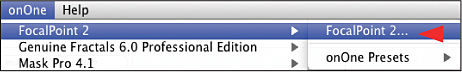
- In the Aperture dialog box, select Round (Figure 1.19.2).
Figure 1.19.2. Select the Round option
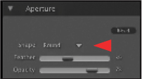
- Click on the FocusBug and center it onto Challen’s face. (Figure 1.19.3).
Figure 1.19.3. Move the FocusBug to the center of her face

- Holding down the Shift key, which locks the FocusBug in place, click on the vertical sizing handle (located at the bottom of the FocusBug). Move the vertical sizing handle until it is just into her hair. I chose a height of 1454 pixels (Figure 1.19.4).
Figure 1.19.4. Moving the vertical size handle to 1454 pixels
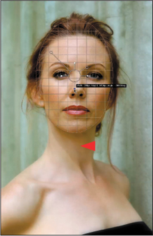
- Holding down the Shift key, which locks the FocusBug in place to ensure that there is no unwanted rotation of the blur effect, click on the horizontal sizing handle (located at the left of the FocusBug) (Figure 1.19.5). Move the vertical sizing handle until it is just into her hair. I chose a width of 982 pixels and my height changed to 1502 pixels (Figure 1.19.6).
Figure 1.19.5. Adjusting the horizontal handle
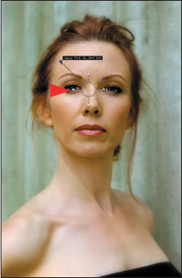
Figure 1.19.6. Changing the height to 1502 pixels
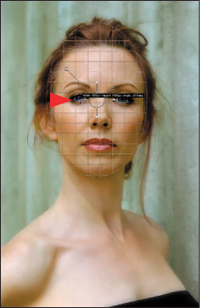
- Click on the Opacity antennae, which I will now refer to as handles (the handle is on a 45° angle located in the upper left of the FocusBug) (Figure 1.19.7). Move the Opacity handle downward until it cannot move anymore, but make sure that it is at its full extension as you do this. You want the Feather amount at 30%. The mask will now look like Figure 1.19.8, and the image looks like Figure 1.19.9.
Figure 1.19.7. Adjusting the Opacity handle
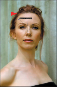
Figure 1.19.8. The mask of the blur
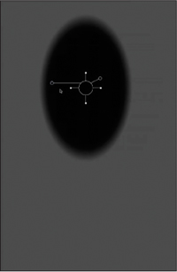
Figure 1.19.9. The image after the initial setup of the FocusBug
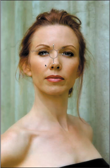
Note
In addition to controlling opacity, by moving the opacity handle up or down you can control the amount of motion in the blur.
To see the mask that you have created, use Command + M / Control + M. To return to the image, repeat the keyboard command.
Once you have the blur circle almost as you want it, you should change the angle and direction from which the blur comes so that it mimics what would have occurred if this was optically created at capture. You could blur the image in post-processing software. You could even create a ratio of 1/3 forward, 2/3 behind the focus plane, but the blur would not look realistic, because it would lack the directional component. Thus, you would create an improbable believability rather than the believable probability that should be your goal.
- Click in the center of the FocusBug, holding down the Option / Alt key, and the FocusBug grid will come up (Figure 1.19.10). Drag the cursor to the right side of the FocusBug grid, slightly below the Opacity handle (Figure 1.19.11).
Figure 1.19.10. Show the grid by holding Option/Alt
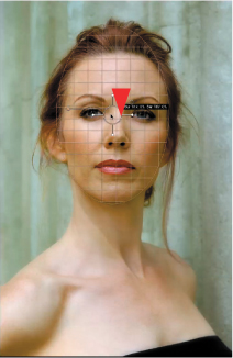
Figure 1.19.11. Drag the grid to the right
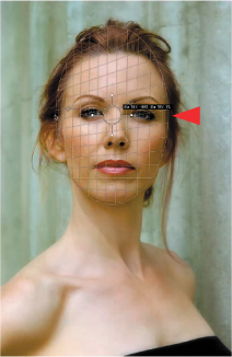
Once you have defined the direction of the blur, you will define the amount. Then you will fine tune the FocalPoint Blur layer by doing some brushwork on a layer mask.
- Click on the Blur handle in the upper right of the FocusBug at a 45° angle to it (Figure 1.19.12). You will now determine how much blur and feather you want. Move the Blur handle in, and slightly downward, until you get a blur of 42% and a feather of 47% (Figure 1.19.13). Click Apply. Compare the before (Figure 1.19.14) and after (Figure 1.19.15).
Figure 1.19.12. Adjust the Blur handle
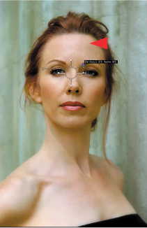
Figure 1.19.13. Move the Blur handle to a blur of 42% and a feather of 47%
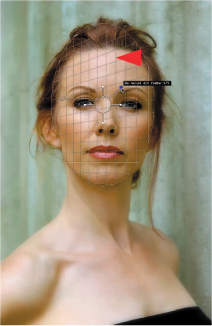
Figure 1.19.14. Before FocalPoint 2
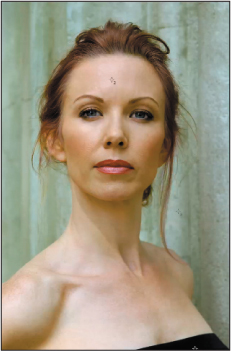
Figure 1.19.15. After FocalPoint 2
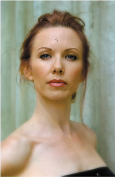
- Hold down Option + D / Alt + D, and click on the Create Layer Mask icon at the bottom of the Layers panel (filling the layer mask with black) in order to add a layer mask to the FocalPoint layer.
- Click D on the Tool bar to get the default colors of white for the foreground and black for Background. Select the Brush tool (keyboard command B) and set the opacity to 50%. (Keyboard command 5 yields an opacity of 50%.) Using the right bracket key ( ] ), increase the brush size to 500 pixels.
- Brush in the entire background, not touching Challen. Bring up the Fade effect dialog box (Command + Shift + F / Control + Shift + F). Lower the amount to 24%. Click OK.
- Starting at the right of the image, just above Challen’s shoulder, brush in the background wall. (Avoid her head and shoulder as much as possible.) Bring up the Fade effect dialog box (Command + Shift + F / Control + Shift + F) and reduce the opacity to 24%. Starting at the top center of the image, brush in the left side of the background wall (still avoiding her head and shoulder). Bring up the Fade effect dialog box and increase the opacity to 75%.
Once you have added angled blur using the FocalPoint software, it is time to add blur to the foreground to mimic what would have occurred if, at the time of capture, you had had a shallow DOF and your focus point had been her eyes.
- Using the left bracket key ( [ ), reduce the brush size to 100 pixels. Brush in just the outline of her neck and shoulders, and then a little in her body.
- Bring up the Fade effect dialog box and lower the opacity to 44%.
- Hold down Option / Alt and click on the layer mask. Sample the color of the area that you have just brushed by Option- / Alt-clicking on that area (Figure 1.19.16). Click on the zero key to give your brush 100% opacity, increase the size of your brush (right bracket key) to 300 pixels, and paint in her neck and chest area (Figure 1.19.17). Compare the image before the layer mask (Figure 1.19.18) and after (Figure 1.19.19).
Figure 1.19.16. Sampling the gray
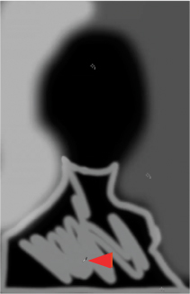
Figure 1.19.17. Painting in her neck and chest
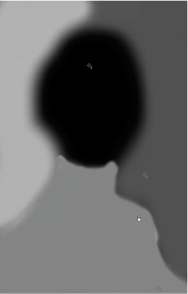
Figure 1.19.18. Before the layer mask
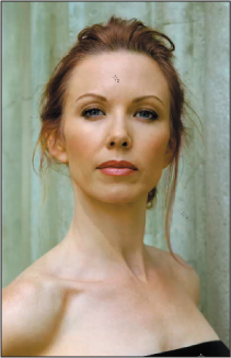
Figure 1.19.19. After the layer mask
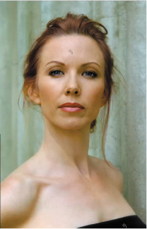
- It is time to re-introduce contrast. Turn on the eyeball of the CONTRAST layer (Blur + Contrast) (Figure 1.19.20).
Figure 1.19.20. Turning the CONTRAST layer on in combination with the blur
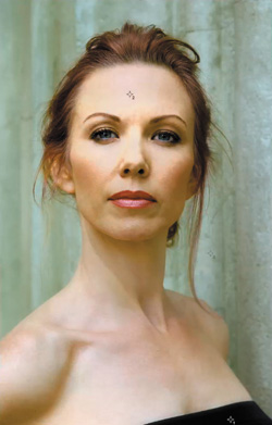
- You should now re-introduce warmth. Turn on the eyeball of the SKYLIGHT layer (Blur + Contrast + Skylight) (Figure 1.19.21).
Figure 1.19.21. Turning the SKYLIGHT layer on
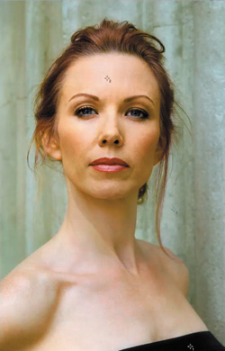
Challen should appear to have moved forward in the image and the wall appeared to move backward.
- Make sure that the top or SKYLIGHT layer is active. Hold down the Shift key and click on the FocalPoint layer. (This will select everything in between these layers.) Make the bottom layer active, and Shift-drag it to the Create a New Layer set. Name the new layer set D_of_F for DOF. Create a master layer, name it MASTER_2 (making sure that MASTER_2 is active), and turn the layer set off.
- Save the file.
Note
When using Smart Filters, it is a good idea to group them in to layer sets, especially when you are using multiple Smart Filters to create a desired effect. When you are done, you can create master layers.
The reason for this is that when opening and saving a file, Photoshop will try to render any Smart Filter that is turned on. This means that you will spend a significant amount of time watching the Technicolor beach ball spin.
By creating a master layer of the combined contents of a layer set, you have a snapshot of everything you have done, and the file will open quite rapidly. The only down side is that you have increased the file’s size.
When I talked about creating the image map for DOF, one of the issues I addressed was that I wanted the back wall to appear lit as if it was positioned well behind the subject. What I actually photographed was a subject standing up against the wall. If I could have cross-lit the background, I would have positioned the subject about five feet away from it. To create a believable probability, I had to add the illusion of optical depth. You will do that by creating a layer of blur between two layers of sharpness.
Everything that you have done thus far is in preparation for working with Render Lighting Effects and Curves in order to lighten and/or darken the image. This will finally create the lighting that I had originally envisioned when I first decided to shoot Challen.