
2. Garbage First Garbage Collector in Depth
This chapter aims at providing in-depth knowledge on the principles supporting HotSpot’s latest garbage collector: the Garbage First garbage collector (referred to as G1 GC for short). These principles were highlighted in Chapter 1, “Garbage First Overview.”
At various points during the narration, concepts like the collection cycles, internal structures, and algorithms will be introduced, followed by comprehensive details. The aim is to document the details without overloading the uninitiated.
To gain the most from the chapter, the reader is expected to be familiar with basic garbage collection concepts and terms and generally how garbage collection works in the Java HotSpot JVM. These concepts and terms include generational garbage collection, the Java heap, young generation space, old generation space, eden space, survivor space, parallel garbage collection, stop-the-world garbage collection, concurrent garbage collection, incremental garbage collection, marking, and compaction. Chapter 1 covers some of these concepts and terms. A good source for additional details is the “HotSpot VM Garbage Collectors” section in Chapter 3, “JVM Overview,” of Java™ Performance [1].
Background
G1 GC is the latest addition to the Java HotSpot Virtual Machine. It is a compacting collector based on the principle of collecting the most garbage first, hence the name “Garbage First” GC. G1 GC has incremental, parallel, stop-the-world pauses that achieve compaction via copying and also has parallel, multistaged concurrent marking that helps in reducing the mark, remark, and cleanup pauses to a bare minimum.
With the introduction of G1 GC, HotSpot JVM moved from the conventional heap layout where the generations are contiguous to generations that are now composed of noncontiguous heap regions. Thus, for an active Java heap, a particular region could be a part of either eden or survivor or old generation, or it could be a humongous region or even just a free region. Multiples of these regions form a “logical” generation to match conventional wisdom formed by previous HotSpot garbage collectors’ idea of generational spaces.
Garbage Collection in G1
G1 GC reclaims most of its heap regions during collection pauses. The only exception to this is the cleanup stage of the multistaged concurrent marking cycle. During the cleanup stage, if G1 GC encounters purely garbage-filled regions, it can immediately reclaim those regions and return them to a linked list of free regions; thus, freeing up those regions does not have to wait for the next garbage collection pause.
G1 GC has three main types of garbage collection cycles: a young collection cycle, a multistage concurrent marking cycle, and a mixed collection cycle. There is also a single-threaded (as of this writing) fallback pause called a “full” garbage collection pause, which is the fail-safe mechanism for G1 GC in case the GC experiences evacuation failures.
Tip
An evacuation failure is also known as a promotion failure or to-space exhaustion or even to-space overflow. The failure usually happens when there is no more free space to promote objects. When faced with such a scenario, all Java HotSpot VM GCs try to expand their heaps. But if the heap is already at its maximum, the GC tries to tenure the regions where objects were successfully copied and update their references. For G1 GC, the objects that could not be copied are tenured in place. All GCs will then have their references self-forwarded. These self-forwarded references are removed at the end of the garbage collection cycle.
During a young collection, G1 GC pauses the application threads to move live objects from the young regions into survivor regions or promote them into old regions or both. For a mixed collection, G1 GC additionally moves live objects from the most (for lack of a better term) “efficient” old regions into free region(s), which become a part of the old generation.
“GC efficiency” actually refers to the ratio of the space to be reclaimed versus the estimated GC cost to collect the region. Due to the lack of a better term, in this book we refer to the sorting of the heap regions in order to identify candidate regions as calculating the “GC efficiency.” The reason for using the same terminology is that GC efficiency evaluates the benefit of collecting a region with respect to the cost of collecting it. And the “efficiency” that we are referring to here is solely dependent on liveness accounting and hence is just the cost of collecting a region. For example, an old region whose collection is less time-consuming than other more expensive old regions is considered to be an “efficient” region. The most efficient regions would be the first ones in the sorted array of regions.
At the end of a collection cycle, the regions that were a part of the collection set or CSet (refer to the section “Collection Sets and Their Importance” later in this chapter for more information) are guaranteed to be free and are returned to the free list. Let’s talk about these concepts in more detail.
The Young Generation
G1 GC is a generational GC comprising the young generation and the old generation. Most allocations, with a few exceptions such as objects too large to fit in the allocating thread’s local allocation buffer (also known as a TLAB) but smaller than what would be considered “humongous,” and of course the “humongous” objects themselves (see the section “Humongous Regions” for more information), by any particular thread will land in that thread’s TLAB. A TLAB enables faster allocations since the owning Java thread is able to allocate in a lock-free manner. These TLABs are from G1 regions that become a part of the young generation. Unless explicitly specified on the command line, the current young generation size is calculated based on the initial and maximum young generation size bounds (as of JDK 8u45 the defaults are 5 percent of the total Java heap for initial young generation size (-XX:G1NewSizePercent) and 60 percent of the total Java heap for maximum young generation size (-XX:G1MaxNewSizePercent) and the pause time goal of the application (-XX:MaxGCPauseMillis).
Tip
G1 GC will select the default of 200ms if -XX:MaxGCPauseMillis is not set on the command line. If the user sets -Xmn or related young generation sizing command-line options such as -XX:NewRatio, G1 GC may not be able to adjust the young generation size based on the pause time goal, and hence the pause time target could become a moot option.
Based on the Java application’s object allocation rate, new free regions are added to the young generation as needed until the desired generation size is met. The heap region size is determined at the launch of the JVM. The heap region size has to be a power of 2 and can range anywhere from 1MB to 32MB. The JVM shoots for approximately 2048 regions and sets the heap region size accordingly (Heap region size = Heap size/2048). The heap region size is aligned and adjusted to fall within the 1MB to 32MB and power of 2 bounds. The adaptive selection of heap region size can be overwritten on the command line by setting it with -XX:G1HeapRegionSize=n. Chapter 3, “Garbage First Garbage Collector Performance Tuning,” includes more information on when to override the JVM’s automatic sizing.
A Young Collection Pause
The young generation consists of G1 GC regions designated as eden regions and G1 GC regions designated as survivor regions. A young collection is triggered when the JVM fails to allocate out of the eden region, that is, the eden is completely filled. The GC then steps in to free some space. The first young collection will move all the live objects from the eden regions into the survivor regions. This is known as “copy to survivor.” From then on, any young collection will promote the live objects from the entire young generation (i.e., eden and survivor regions) into new regions that are now the new survivor regions. The young collections will also occasionally promote a few objects into regions out of the old generation when they survive a predetermined promotion threshold. This is called “aging” the live objects. The promotion of the live objects from the young generation into the old generation is called “tenuring” the objects, and consequently the age threshold is called the “tenuring threshold.” The promotion of objects into the survivor regions or into the old generation happens in the promoting GC thread’s local allocation buffer (also known as Promotion Lab, or PLAB for short). There is a per-GC-thread PLAB for the survivor regions and for the old generation.
During every young collection pause, G1 GC calculates the amount of expansion or contraction to be performed on the current young generation size (i.e., G1 GC decides to either add or remove free regions) based on the total time that it took to perform the current collection; the size of the remembered sets or RSets (more on this in the section “Remembered Sets and Their Importance” later in this chapter); the current, the maximum, and the minimum young generation capacity; and the pause time target. Thus the young generation is resized at the end of a collection pause. The previous and the next sizes of the young generation can be observed and calculated by looking at the output of -XX:+PrintGCDetails. Let’s look at an example. (Note that throughout this book lines of output have been wrapped in order to fit on the book page.)
15.894: [GC pause (G1 Evacuation Pause) (young), 0.0149364 secs]
[Parallel Time: 9.8 ms, GC Workers: 8]
<snip>
[Code Root Fixup: 0.1 ms]
[Code Root Purge: 0.0 ms]
[Clear CT: 0.2 ms]
[Other: 4.9 ms]
<snip>
[Eden: 695.0M(695.0M)->0.0B(1043.0M) Survivors: 10.0M->13.0M Heap:
748.5M(1176.0M)->57.0M(1760.0M)]
[Times: user=0.08 sys=0.00, real=0.01 secs]
Here the new size of the young generation can be calculated by adding the new Eden size to the new Survivors size (i.e., 1043M + 13M = 1056M).
Object Aging and the Old Generation
As was covered briefly in the previous section, “A Young Collection Pause,” during every young collection, G1 GC maintains the age field per object. The current total number of young collections that any particular object survives is called the “age” of that object. The GC maintains the age information, along with the total size of the objects that have been promoted into that age, in a table called the “age table.” Based on the age table, the survivor size, the survivor fill capacity (determined by the -XX:TargetSurvivorRatio (default = 50)), and the -XX:MaxTenuringThreshold (default = 15), the JVM adaptively sets a tenuring threshold for all surviving objects. Once the objects cross this tenuring threshold, they get promoted/tenured into the old generation regions. When these tenured objects die in the old generation, their space can be freed by a mixed collection, or during cleanup (but only if the entire region can be reclaimed), or, as a last resort, during a full garbage collection.
Humongous Regions
For the G1 GC, the unit of collection is a region. Hence, the heap region size (-XX:G1HeapRegionSize) is an important parameter since it determines what size objects can fit into a region. The heap region size also determines what objects are characterized as “humongous.” Humongous objects are very large objects that span 50 percent or more of a G1 GC region. Such an object doesn’t follow the usual fast allocation path and instead gets allocated directly out of the old generation in regions marked as humongous regions.
Figure 2.1 illustrates a contiguous Java heap with the different types of G1 regions identified: young region, old region, and humongous region. Here, we can see that each of the young and old regions spans one unit of collection. The humongous region, on the other hand, spans two units of collection, indicating that humongous regions are formed of contiguous heap regions. Let’s look a little deeper into three different humongous regions.

In Figure 2.2, Humongous Object 1 spans two contiguous regions. The first contiguous region is labeled “StartsHumongous,” and the consecutive contiguous region is labeled “ContinuesHumongous.” Also illustrated in Figure 2.2, Humongous Object 2 spans three contiguous heap regions, and Humongous Object 3 spans just one region.

Tip
Past studies of these humongous objects have indicated that the allocations of such objects are rare and that the objects themselves are long-lived. Another good point to remember is that the humongous regions need to be contiguous (as shown in Figure 2.2). Hence it makes no sense to move them since there is no gain (no space reclamation), and it is very expensive since large memory copies are not trivial in expense. Hence, in an effort to avoid the copying expense of these humongous objects during young garbage collections, it was deemed better to directly allocate the humongous objects out of the old generation. But in recent years, there are many transaction-type applications that may have not-so-long-lived humongous objects. Hence, various efforts are being made to optimize the allocation and reclamation of humongous objects.
As mentioned earlier, humongous objects follow a separate and quite involved allocation path. This means the humongous object allocation path doesn’t take advantage of any of the young generation TLABs and PLABs that are optimized for allocation or promotion, since the cost of zeroing the newly allocated object would be massive and probably would circumvent any allocation path optimization gain. Another noteworthy difference in the handling of humongous objects is in the collection of humongous regions. Prior to JDK 8u40, if any humongous region was completely free, it could be collected only during the cleanup pause of the concurrent collection cycle. In an effort to optimize the collection of short-lived humongous objects, JDK 8u40 made a noteworthy change such that if the humongous regions are determined to have no incoming references, they can be reclaimed and returned to the list of free regions during a young collection. A full garbage collection pause will also collect completely free humongous regions.
Tip
An important potential issue or confusion needs to be highlighted here. Say the current G1 region size is 2MB. And say that the length of a byte array is aligned at 1MB. This byte array will still be considered a humongous object and will need to be allocated as such, since the 1MB array length doesn’t include the array’s object header size.
A Mixed Collection Pause
As more and more objects get promoted into the old regions or when humongous objects get allocated into the humongous regions, the occupancy of the old generation and hence the total occupied Java heap increases. In order to avoid running out of heap space, the JVM process needs to initiate a garbage collection that not only covers the regions in the young generation but also adds some old regions to the mix. Refer to the previous section on humongous regions to read about the special handling (allocation and reclamation) of humongous objects.
In order to identify old regions with the most garbage, G1 GC initiates a concurrent marking cycle, which helps with marking roots and eventually identifying all live objects and also calculating the liveness factor per region. There needs to be a delicate balance between the rate of allocations and promotions and the triggering of this marking cycle such that the JVM process doesn’t run out of Java heap space. Hence, an occupancy threshold is set at the start of the JVM process. As of this writing and up through at least JDK 8u45 this occupancy threshold is not adaptive and can be set by the command-line option -XX:InitiatingHeapOccupancyPercent (which I very fondly call IHOP).
Tip
In G1, the IHOP threshold defaults to 45 percent of the total Java heap. It is important to note that this heap occupancy percentage applies to the entire Java heap, unlike the heap occupancy command-line option used with CMS GC where it applies only to the old generation. In G1 GC, there is no physically separate old generation—there is a single pool of free regions that can be allocated as eden, survivor, old, or humongous. Also, the number of regions that are allocated, for say the eden, can vary over time. Hence having an old generation percentage didn’t really make sense.
When the old generation occupancy reaches (or exceeds) the IHOP threshold, a concurrent marking cycle is initiated. Toward the end of marking, G1 GC calculates the amount of live objects per old region. Also, during the cleanup stage, G1 GC ranks the old regions based on their “GC efficiency.” Now a mixed collection can happen! During a mixed collection pause, G1 GC not only collects all of the regions in the young generation but also collects a few candidate old regions such that the old regions with the most garbage are reclaimed.
Tip
An important point to keep in mind when comparing CMS and G1 logs is that the multistaged concurrent cycle in G1 has fewer stages than the multistaged concurrent cycle in CMS.
A single mixed collection is similar to a young collection pause and achieves compaction of the live objects via copying. The only difference is that during a mixed collection, the collection set also incorporates a few efficient old regions. Depending on a few parameters (as discussed later in this chapter), there could be more than one mixed collection pause. This is called a “mixed collection cycle.” A mixed collection cycle can happen only after the marking/IHOP threshold is crossed and after the completion of a concurrent marking cycle.
There are two important parameters that help determine the total number of mixed collections in a mixed collection cycle: -XX:G1MixedGCCountTarget and -XX:G1HeapWastePercent.
-XX:G1MixedGCCountTarget, which defaults to 8 (JDK 8u45), is the mixed GC count target option whose intent is to set a physical limit on the number of mixed collections that will happen after the marking cycle is complete. G1 GC divides the total number of candidate old regions available for collection by the count target number and sets that as the minimum number of old regions to be collected per mixed collection pause. This can be represented as an equation as follows:
Minimum old CSet per mixed collection pause = Total number of candidate old regions identified for mixed collection cycle/G1MixedGCCountTarget
-XX:G1HeapWastePercent, which defaults to 5 percent (JDK 8u45) of the total Java heap, is an important parameter that controls the number of old regions to be collected during a mixed collection cycle. For every mixed collection pause, G1 GC identifies the amount of reclaimable heap based on the dead object space that can be reclaimed. As soon as G1 GC reaches this heap waste threshold percentage, G1 GC stops the initiation of a mixed collection pause, thus culminating the mixed collection cycle. Setting the heap waste percent basically helps with limiting the amount of heap that you are willing to waste to effectively speed up the mixed collection cycle.
Thus the number of mixed collections per mixed collection cycle can be controlled by the minimum old generation CSet per mixed collection pause count and the heap waste percentage.
Collection Sets and Their Importance
During any garbage collection pause all the regions in the CSet are freed. A CSet is a set of regions that are targeted for reclamation during a garbage collection pause. All live objects in these candidate regions will be evacuated during a collection, and the regions will be returned to a list of free regions. During a young collection, the CSet can contain only young regions for collection. A mixed collection, on the other hand, will not only add all the young regions but also add some old candidate regions (based on their GC efficiency) to its CSet.
There are two important parameters that help with the selection of candidate old regions for the CSet of a mixed collection: -XX:G1MixedGCLiveThresholdPercent and -XX:G1OldCSetRegionThresholdPercent.
-XX:G1MixedGCLiveThresholdPercent, which defaults to 85 percent (JDK 8u45) of a G1 GC region, is a liveness threshold and a set limit to exclude the most expensive of old regions from the CSet of mixed collections. G1 GC sets a limit such that any old region that falls below this liveness threshold is included in the CSet of a mixed collection.
-XX:G1OldCSetRegionThresholdPercent, which defaults to 10 percent (JDK 8u45) of the total Java heap, sets the maximum limit on the number of old regions that can be collected per mixed collection pause. The threshold is dependent on the total Java heap available to the JVM process and is expressed as a percentage of the total Java heap. Chapter 3 covers a few examples to highlight the functioning of these thresholds.
Remembered Sets and Their Importance
A generational collector segregates objects in different areas in the heap according to the age of those objects. These different areas in the heap are referred to as the generations. The generational collector then can concentrate most of its collection effort on the most recently allocated objects because it expects to find most of them dead sooner rather than later. These generations in the heap can be collected independently. The independent collection helps lower the response times since the GC doesn’t have to scan the entire heap, and also (e.g., in the case of copying generational collectors) older long-lived objects don’t have to be copied back and forth, thus reducing the copying and reference updating overhead.
In order to facilitate the independence of collections, many garbage collectors maintain RSets for their generations. An RSet is a data structure that helps maintain and track references into its own unit of collection (which in G1 GC’s case is a region), thus eliminating the need to scan the entire heap for such information. When G1 GC executes a stop-the-world collection (young or mixed), it scans through the RSets of regions contained in its CSet. Once the live objects in the region are moved, their incoming references are updated.
With G1 GC, during any young or mixed collection, the young generation is always collected in its entirety, eliminating the need to track references whose containing object resides in the young generation. This reduces the RSet overhead. Thus, G1 GC just needs to maintain the RSets in the following two scenarios:
![]() Old-to-young references—G1 GC maintains pointers from regions in the old generation into the young generation region. The young generation region is said to “own” the RSet and hence the region is said to be an RSet “owning” region.
Old-to-young references—G1 GC maintains pointers from regions in the old generation into the young generation region. The young generation region is said to “own” the RSet and hence the region is said to be an RSet “owning” region.
![]() Old-to-old references—Here pointers from different regions in the old generation will be maintained in the RSet of the “owning” old generation region.
Old-to-old references—Here pointers from different regions in the old generation will be maintained in the RSet of the “owning” old generation region.
In Figure 2.3, we can see one young region (Region x) and two old regions (Region y and Region z). Region x has an incoming reference from Region z. This reference is noted in the RSet for Region x. We also observe that Region z has two incoming references, one from Region x and another from Region y. The RSet for Region z needs to note only the incoming reference from Region y and doesn’t have to remember the reference from Region x, since, as explained earlier, young generation is always collected in its entirety. Finally, for Region y, we see an incoming reference from Region x, which is not noted in the RSet for Region y since Region x is a young region.

As shown in Figure 2.3, there is only one RSet per region. Depending on the application, it could be that a particular region (and thus its RSet) could be “popular” such that there could be many updates in the same region or even to the same location. This is not that uncommon in Java applications.
G1 GC has its way of handling such demands of popularity; it does so by changing the density of RSets. The density of RSets follows three levels of granularity, namely, sparse, fine, and coarse. For a popular region, the RSet would probably get coarsened to accommodate the pointers from various other regions. This will be reflected in the RSet scanning time for those regions. (Refer to Chapter 3 for more details on RSet scanning times.) Each of the three granular levels has a per-region-table (PRT) abstract housing for any particular RSet.
Since G1 GC regions are internally further divided into chunks, at the G1 GC region level the lowest granularity achievable is a 512-byte heap chunk called a “card” (refer to Figure 2.4). A global card table maintains all the cards.

When a pointer makes a reference to an RSet’s owning region, the card containing that pointer is noted in the PRT. A sparse PRT is basically a hash table of those card indices. This simple implementation leads to faster scan times by the garbage collector. On the other hand, fine-grained PRT and coarse-grained bitmap are handled in a different manner. For fine-grained PRT, each entry in its open hash table corresponds to a region (with a reference into the owning region) where the card indices within that region are stored in a bitmap. There is a maximum limit to the fine-grained PRT, and when it is exceeded, a bit (called the “coarse-grained bit”) is set in the coarse-grained bitmap. Once the coarse-grained bit is set, the corresponding entry in the fine-grained PRT is deleted. The coarse-grained bitmap is simply a bitmap with one bit per region such that a set bit means that the corresponding region might contain a reference to the owning region. So then the entire region associated with the set bit must be scanned to find the reference. Hence a remembered set coarsened to a coarse-grained bitmap is the slowest to scan for the garbage collector. More details on this can be found in Chapter 3.
During any collection cycle, when scanning the remembered sets and thus the cards in the PRT, G1 GC will mark the corresponding entry in the global card table to avoid rescanning that card. At the end of the collection cycle this card table is cleared; this is shown in the GC output (printed with -XX:+PrintGCDetails) as Clear CT and is next in sequence to the parallel work done by the GC threads (i.e., external root scanning, updating and scanning the remembered sets, object copying, and termination protocol). There are also other sequential activities such as choosing and freeing the CSet and also reference processing and enqueuing. Here is sample output using -XX:+UseG1GC -XX:PrintGCDetails -XX:PrintGCTimeStamps with build JDK 8u45. The RSet and card table activities are highlighted. More details on the output are covered in Chapter 3.
12.664: [GC pause (G1 Evacuation Pause) (young), 0.0010649 secs]
[Parallel Time: 0.5 ms, GC Workers: 8]
[GC Worker Start (ms): Min: 12664.1, Avg: 12664.2, Max:
12664.2, Diff: 0.1]
[Ext Root Scanning (ms): Min: 0.2, Avg: 0.3, Max: 0.3, Diff:
0.1, Sum: 2.1]
[Update RS (ms): Min: 0.0, Avg: 0.0, Max: 0.0, Diff: 0.0, Sum: 0.2]
[Processed Buffers: Min: 1, Avg: 1.1, Max: 2, Diff: 1, Sum: 9]
[Scan RS (ms): Min: 0.0, Avg: 0.0, Max: 0.0, Diff: 0.0, Sum: 0.1]
[Code Root Scanning (ms): Min: 0.0, Avg: 0.0, Max: 0.0, Diff: 0.0,
Sum: 0.0]
[Object Copy (ms): Min: 0.0, Avg: 0.0, Max: 0.1, Diff: 0.0,
Sum: 0.4]
[Termination (ms): Min: 0.0, Avg: 0.0, Max: 0.0, Diff: 0.0,
Sum: 0.0]
[GC Worker Other (ms): Min: 0.0, Avg: 0.0, Max: 0.0, Diff: 0.0,
Sum: 0.1]
[GC Worker Total (ms): Min: 0.3, Avg: 0.4, Max: 0.4, Diff: 0.1,
Sum: 2.9]
[GC Worker End (ms): Min: 12664.5, Avg: 12664.5, Max: 12664.5,
Diff: 0.0]
[Code Root Fixup: 0.0 ms]
[Code Root Purge: 0.0 ms]
[Clear CT: 0.1 ms]
[Other: 0.4 ms]
[Choose CSet: 0.0 ms]
[Ref Proc: 0.2 ms]
[Ref Enq: 0.0 ms]
[Redirty Cards: 0.1 ms]
[Humongous Reclaim: 0.0 ms]
[Free CSet: 0.1 ms]
[Eden: 83.0M(83.0M)->0.0B(83.0M) Survivors: 1024.0K->1024.0K Heap:
104.0M(140.0M)->21.0M(140.0M)]
[Times: user=0.00 sys=0.00, real=0.01 secs]
Concurrent Refinement Threads and Barriers
The advanced RSet structure comes with its own maintenance costs in the form of write barriers and concurrent “refinement” threads.
Barriers are snippets of native code that are executed when certain statements in a managed runtime are executed. The use of barriers in garbage collection algorithms is well established, and so is the cost associated with executing the barrier code since the native instruction path length increases.
OpenJDK HotSpot’s Parallel Old and CMS GCs use a write barrier that executes when the HotSpot JVM performs an object reference write operation:
object.field = some_other_object;
The barrier updates a card-table-type structure [2] to track intergenerational references. The card table is scanned during minor garbage collections. The write barrier algorithm is based on Urs Hölzle’s fast write barrier [3], which reduces the barrier overhead to just two extra instructions in the compiled code.
G1 GC employs a pre-write and a post-write barrier. The former is executed before the actual application assignment takes place and is covered in detail in the concurrent marking section, while the latter is executed after the assignment and is further described here.
G1 GC issues a write barrier anytime a reference is updated. For example, consider the update in this pseudo-code:
object.field = some_other_object;
This assignment will trigger the barrier code. Since the barrier is issued after a write to any reference, it is called a “post-write” barrier. Write barrier instruction sequences can get very expensive, and the throughput of the application will fall proportionally with the complexity of the barrier code; hence G1 GC does the minimum amount of work that is needed to figure out if the reference update is a cross-region update since a cross-region reference update needs to be captured in the RSet of the owning region. For G1 GC, the barrier code includes a filtering technique briefly discussed in “Older-First Garbage Collection in Practice” [4] that involves a simple check which evaluates to zero when the update is in the same region. The following pseudo-code illustrates G1 GC’s write barrier:
(&object.field XOR &some_other_object) >> RegionSize
Anytime a cross-region update happens, G1 GC will enqueue the corresponding card in a buffer called the “update log buffer” or “dirty card queue.” In our update example, the card containing object is logged in the update log buffer.
Tip
The concurrent refinement threads are threads dedicated to the sole purpose of maintaining the remembered sets by scanning the logged cards in the filled log buffers and then updating the remembered set for those regions. The maximum number of refinement threads is determined by –XX:G1ConcRefinementThreads. As of JDK 8u45, if –XX:G1ConcRefinementThreads is not set on the command line, it is ergonomically set to be the same as –XX:ParallelGCThreads.
Once the update log buffer reaches its holding capacity, it is retired and a new log buffer is allocated. The card enqueuing then happens in this new buffer. The retired buffer is placed in a global list. Once the refinement threads find entries in the global list, they start concurrently processing the retired buffers. The refinement threads are always active, albeit initially only a few of them are available. G1 GC handles the deployment of the concurrent refinement threads in a tiered fashion, adding more threads to keep up with the amount of filled log buffers. Activation thresholds are set by the following flags: -XX:G1ConcRefinementGreenZone, -XX:G1ConcRefinementYellowZone, and -XX:G1ConcRefinementRedZone. If the concurrent refinement threads can’t keep up with the number of filled buffers, mutator threads are enlisted for help. At such a time, the mutator threads will stop their work and help the concurrent refinement threads to finish processing the filled log buffers. Mutator threads in GC terminology are the Java application threads. Hence, when the concurrent refinement threads can’t keep up the number of filled buffers, the Java application will be halted until the filled log buffers are processed. Thus, measures should be taken to avoid such a scenario.
Users are not expected to manually tune any of the three refinement zones. There may be rare occasions when it makes sense to tune –XX:G1ConcRefinementThreads or –XX:ParallelGCThreads. Chapter 3 explains more about concurrent refinement and the refinement threads.
Concurrent Marking in G1 GC
With the introduction of G1 GC regions and liveness accounting per region, it became clear that an incremental and complete concurrent marking algorithm was required. Taiichi Yuasa presented an algorithm for incremental mark and sweep GC in which he employed a “snapshot-at-the-beginning” (SATB) marking algorithm [5].
Yuasa’s SATB marking optimization concentrated on the concurrent marking phase of the mark-sweep GC. The SATB marking algorithm was well suited for G1 GC’s regionalized heap structure and addressed a major complaint about the HotSpot JVM’s CMS GC algorithm—the potential for lengthy remark pauses.
G1 GC establishes a marking threshold which is expressed as a percentage of the total Java heap and defaults to 45 percent. This threshold, which can be set at the command line using the -XX:InitiatingHeapOccupancyPercent (IHOP) option, when crossed, will initiate the concurrent marking cycle. The marking task is divided into chunks such that most of the work is done concurrently while the mutator threads are active. The goal is to have the entire Java heap marked before it reaches its full capacity.
The SATB algorithm simply creates an object graph that is a logical “snapshot” of the heap. SATB marking guarantees that all garbage objects that are present at the start of the concurrent marking phase will be identified by the snapshot. Objects allocated during the concurrent marking phase will be considered live, but they are not traced, thus reducing the marking overhead. The technique guarantees that all live objects that were alive at the start of the marking phase are marked and traced, and any new allocations made by the concurrent mutator threads during the marking cycle are marked as live and consequently not collected.
The marking data structures contain just two bitmaps: previous and next. The previous bitmap holds the last complete marking information. The current marking cycle creates and updates the next bitmap. As time passes, the previous marking information becomes more and more stale. Eventually, the next bitmap will replace the previous bitmap at the completion of the marking cycle.
Corresponding to the previous bitmap and the next bitmap, each G1 GC heap region has two top-at-mark-start (TAMS) fields respectively called previous TAMS (or PTAMS) and next TAMS (or NTAMS). The TAMS fields are useful in identifying objects allocated during a marking cycle.
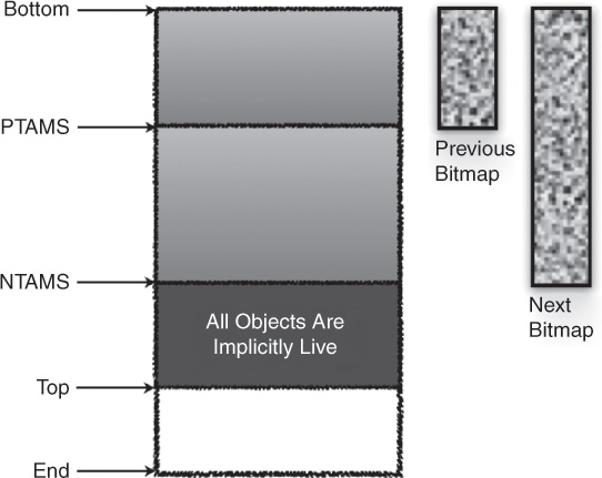
At the start of a marking cycle, the NTAMS field is set to the current top of each region as shown in Figure 2.5. Objects that are allocated (or have died) since the start of the marking cycle are located above the corresponding TAMS value and are considered to be implicitly live. Live objects below TAMS need to be explicitly marked. Let’s walk through an example: In Figure 2.6, we see a heap region during concurrent marking, with “Previous Bitmap,” “Next Bitmap,” “PTAMS,” “NTAMS,” and “Top” as indicated. Live objects between PTAMS and the bottom (indicated as “Bottom” in the figures) of the heap are all marked and held in the previous bitmap as indicated in Figure 2.7. All objects between PTAMS and the top of the heap region are implicitly live (with respect to the previous bitmap) as shown in Figure 2.8. These include the objects allocated during the concurrent marking and are thus allocated above the NTAMS and are implicitly live with respect to the next bitmap, as shown in Figure 2.10. At the end of the remark pause, all live objects above the PTAMS and below the NTAMS are completely marked as shown in Figure 2.9. As mentioned earlier, objects allocated during the concurrent marking cycle will be allocated above the NTAMS and are considered implicitly live with respect to the next bitmap (see Figure 2.10).

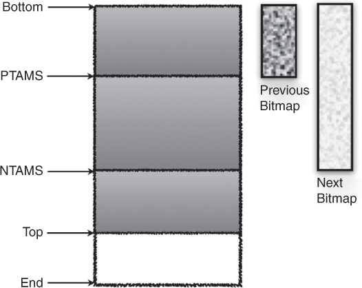
Figure 2.6 A heap region showing previous bitmap, next bitmap, PTAMS, and NTAMS during concurrent marking


Stages of Concurrent Marking
The marking task chunks are carried out mostly concurrently. A few tasks are completed during short stop-the-world pauses. Let’s now talk about the significance of these tasks.
Initial Mark
During initial mark, the mutator threads are stopped in order to facilitate the marking of all the objects in the Java heap that are directly reachable by the roots (also called root objects).
Tip
Root objects are objects that are reachable from outside of the Java heap; native stack objects and JNI (Java Native Interface) local or global objects are some examples.
Since the mutator threads are stopped, the initial-mark stage is a stop-the-world phase. Also, since young collection also traces roots and is stop-the-world, it’s convenient (and time efficient) to carry out initial marking at the same time as a regular young collection. This is also known as “piggybacking.” During the initial-mark pause, the NTAMS value for each region is set to the current top of the region (see Figure 2.5). This is done iteratively until all the regions of the heap are processed.
Root Region Scanning
After setting the TAMS for each region, the mutator threads are restarted, and the G1 GC now works concurrently with the mutator threads. For the correctness of the marking algorithm, the objects copied to the survivor regions during the initial-mark young collection need to be scanned and considered as marking roots. G1 GC hence starts scanning the survivor regions. Any object that is referenced from the survivor regions is marked. Because of this, the survivor regions that are scanned in this manner are referred to as “root regions.”
The root region scanning stage must complete before the next garbage collection pause since all objects that are referenced from the survivor regions need to be identified and marked before the entire heap can be scanned for live objects.
Concurrent Marking
The concurrent marking stage is concurrent and multithreaded. The command-line option to set the number of concurrent threads to be used is -XX:ConcGCThreads. By default, G1 GC sets the total number of threads to one-fourth of the parallel GC threads (-XX:ParallelGCThreads). The parallel GC threads are calculated by the JVM at the start of the VM. The concurrent threads scan a region at a time and use the “finger” pointer optimization to claim that region. This “finger” pointer optimization is similar to CMS GC’s “finger” optimization and can be studied in [2].
As mentioned in the “RSets and Their Importance” section, G1 GC also employs a pre-write barrier to perform actions required by the SATB concurrent marking algorithm. As an application mutates its object graph, objects that were reachable at the start of marking and were a part of the snapshot may be overwritten before they are discovered and traced by a marking thread. Hence the SATB marking guarantee requires that the modifying mutator thread log the previous value of the pointer that needs to be modified, in an SATB log queue/buffer. This is called the “concurrent marking/SATB pre-write barrier” since the barrier code is executed before the update. The pre-write barrier enables the recording of the previous value of the object reference field so that concurrent marking can mark through the object whose value is being overwritten.
The pseudo-code of the pre-write barrier for an assignment of the form x.f := y is as follows:
if (marking_is_active) {
pre_val := x.f;
if (pre_val != NULL) {
satb_enqueue(pre_val);
}
}
The marking_is_active condition is a simple check of a thread-local flag that is set to true at the start of marking, during the initial-mark pause. Guarding the rest of the pre-barrier code with this check reduces the overhead of executing the remainder of the barrier code when marking is not active. Since the flag is thread-local and its value may be loaded multiple times, it is likely that any individual check will hit in cache, further reducing the overhead of the barrier.
The satb_enqueue() first tries to enqueue the previous value in a thread-local buffer, referred to as an SATB buffer. The initial size of an SATB buffer is 256 entries, and each application thread has an SATB buffer. If there is no room to place the pre_val in the SATB buffer, the JVM runtime is called; the thread’s current SATB buffer is retired and placed onto a global list of filled SATB buffers, a new SATB buffer is allocated for the thread, and the pre_val is recorded. It is the job of the concurrent marking threads to check and process the filled buffers at regular intervals to enable the marking of the logged objects.
The filled SATB buffers are processed (during the marking stage) from the global list by iterating through each buffer and marking each recorded object by setting the corresponding bit in the marking bitmap (and pushing the object onto a local marking stack if the object lies behind the finger). Marking then iterates over the set bits in a section of the marking bitmap, tracing the field references of the marked objects, setting more bits in the marking bitmap, and pushing objects as necessary.
Live data accounting is piggybacked on the marking operation. Hence, every time an object is marked, it is also counted (i.e., its bytes are added to the region’s total). Only objects below NTAMS are marked and counted. At the end of this stage, the next marking bitmap is cleared so that it is ready when the next marking cycle starts. This is done concurrently with the mutator threads.
Tip
JDK 8u40 introduces a new command-line option -XX:+ClassUnloadingWithConcurrentMark which, by default, enables class unloading with concurrent marking. Hence, concurrent marking can track classes and calculate their liveness. And during the remark stage, the unreachable classes can be unloaded.
Remark
The remark stage is the final marking stage. During this stop-the-world stage, G1 GC completely drains any remaining SATB log buffers and processes any updates. G1 GC also traverses any unvisited live objects. As of JDK 8u40, the remark stage is stop-the-world, since mutator threads are responsible for updating the SATB log buffers and as such “own” those buffers. Hence, a final stop-the-world pause is necessary to cover all the live data and safely complete live data accounting. In order to reduce time spent in this pause, multiple GC threads are used to parallel process the log buffers. The -XX:ParallelGCThreads help set the number of GC threads available during any GC pause. Reference processing is also a part of the remark stage.
Tip
Any application that heavily uses reference objects (weak references, soft references, phantom references, or final references) may see high remark times as a result of the reference-processing overhead. We will learn more about this in Chapter 3.
Cleanup
During the cleanup pause, the two marking bitmaps swap roles: the next marking bitmap becomes the previous one (given that the current marking cycle has been finalized and the next marking bitmap now has consistent marking information), and the previous marking bitmap becomes the next one (which will be used as the current marking bitmap during the next cycle). Similarly, PTAMS and NTAMS swap roles as well. Three major contributions of the cleanup pause are identifying completely free regions, sorting the heap regions to identify efficient old regions for mixed garbage collection, and RSet scrubbing. Current heuristics rank the regions according to liveness (the regions that have a lot of live objects are really expensive to collect, since copying is an expensive operation) and remembered set size (again, regions with large remembered sets are expensive to collect due to the regions’ popularity—the concept of popularity was discussed in the “RSets and Their Importance” section). The goal is to collect/evacuate the candidate regions that are deemed less expensive (fewer live objects and less popular) first.
An advantage of identifying the live objects in each region is that on encountering a completely free region (that is, a region with no live objects), its remembered set can be cleared and the region can be immediately reclaimed and returned to the list of free regions instead of being placed in the GC-efficient (the concept of GC efficiency was discussed in the “Garbage Collection in G1” section) sorted array and having to wait for a reclamation (mixed) garbage collection pause. RSet scrubbing also helps detect stale references. So, for example, if marking finds that all the objects on a particular card are dead, the entry for that particular card is purged from the “owning” RSet.
Evacuation Failures and Full Collection
Sometimes G1 GC is unable to find a free region when trying to copy live objects from a young region or when trying to copy live objects during evacuation from an old region. Such a failure is reported as a to-space exhausted failure in the GC logs, and the duration of the failure is shown further down in the log as the Evacuation Failure time (331.5ms in the following example):
111.912: [GC pause (G1 Evacuation Pause) (young) (to-space exhausted),
0.6773162 secs]
<snip>
[Evacuation Failure: 331.5 ms]
There are other times when a humongous allocation may not be able to find contiguous regions in the old generation for allocating humongous objects.
At such times, the G1 GC will attempt to increase its usage of the Java heap. If the expansion of the Java heap space is unsuccessful, G1 GC triggers its fail-safe mechanism and falls back to a serial (single-threaded) full collection.
During a full collection, a single thread operates over the entire heap and does mark, sweep, and compaction of all the regions (expensive or otherwise) constituting the generations. After completion of the collection, the resultant heap now consists of purely live objects, and all the generations have been fully compacted.
Tip
Prior to JDK 8u40, unloading of classes was possible only at a full collection.
The single-threaded nature of the serial full collection and the fact that the collection spans the entire heap can make this a very expensive collection, especially if the heap size is fairly large. Hence, it is highly recommended that a nontrivial tuning exercise be done in such cases where full collections are a frequent occurrence.
References
[1] Charlie Hunt and Binu John. Java™ Performance. Addison-Wesley, Upper Saddle River, NJ, 2012. ISBN 978-0-13-714252-1.
[2] Tony Printezis and David Detlefs. “A Generational Mostly-Concurrent Garbage Collector.” Proceedings of the 2nd International Symposium on Memory Management. ACM, New York, 2000, pp. 143–54. ISBN 1-58113-263-8.
[3] Urs Hölzle. “A Fast Write Barrier for Generational Garbage Collectors.” Presented at the OOPSLA’93 Garbage Collection Workshop, Washington, DC, October 1993.
[4] Darko Stefanovic, Matthew Hertz, Stephen M. Blackburn, Kathryn S McKinley, and J. Eliot B. Moss. “Older-First Garbage Collection in Practice: Evaluation in a Java Virtual Machine.” Proceedings of the 2002 Workshop on Memory System Performance. ACM, New York, 2002, pp. 25–36.
[5] Taiichi Yuasa. “Real-Time Garbage Collection on General Purpose Machines.” Journal of Systems and Software, Volume 11, Issue 3, March 1990, pp. 181–98. Elsevier Science, Inc., New York.