
5
Real Options Valuation
Uncertainty can sometimes be a source of additional value, especially to those who are poised to take advantage of it. The approaches we have described in the last three chapters for assessing the value of an asset are mainly focused on the negative effects of risk. Put another way, they are all focused on the downside of risk; they miss the opportunity component that provides the upside. The real options approach is the only one that gives prominence to the upside potential for risk.
We begin this chapter by describing in very general terms the argument behind the real options approach, noting its foundations in two elements:
The capacity of individuals or entities to learn from what is happening around them
Their willingness and ability to modify their behavior based on that learning
We then describe the various forms that real options can take in practice and how they can affect how we assess the value of investments and our behavior. The last section considers some of the potential pitfalls of using the real options argument and how it can be best incorporated into a portfolio of risk-assessment tools. Because the chapter assumes some familiarity with option payoffs and option pricing, we provide a short overview of both in the appendix at the end of this chapter.
The Essence of Real Options
To understand the basis of the real options argument and the reasons for its allure, it is easiest to go back to the risk-assessment tool unveiled in Chapter 3—decision trees. Figure 5.1 shows a simple example of a decision tree.
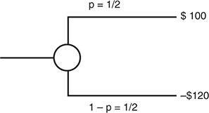
Given the equal probabilities of up and down movements, and the larger potential loss, the expected value for this investment is negative:
Expected Value = 0.50 (100) + 0.5 (–120) = –$10
Now contrast this with the slightly more complicated two-phase decision tree shown in Figure 5.2.
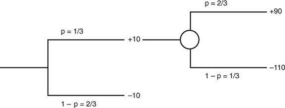
Note that the total potential profits and losses over the two phases in the tree are identical to the profit and loss of the simple tree shown in Figure 5.1; your total gain is $100, and your total loss is $120. Note also that the cumulative probabilities of success and failure remain at the 50% we used in the simple tree. When we compute the expected value of this tree, though, the outcome changes:
Expected Value = (2/3) (–10) + 1/3 [10 + (2/3)(90) + (1/3)(–110)] = $4.44
What is it about the second decision tree that makes a potentially bad investment (in the first tree) into a good investment (in the second)? We can attribute the change to two factors. First, by allowing for an initial phase where you get to observe the cash flows on a first and relatively small try at the investment, we allow for learning. Thus, getting a bad outcome in the first phase (−10 instead of +10) is an indicator that the overall investment is more likely to be money-losing than money-making. Second, you act on the learning by abandoning the investment if the outcome from the first phase is negative; we will call this adaptive behavior.
In essence, the value of real options stems from the fact that when investing in risky assets, we can learn from observing what happens in the real world. We can adapt our behavior to increase our potential upside from the investment and decrease the possible downside. In the real options framework, we use updated knowledge or information to expand opportunities while reducing danger. In the context of a risky investment, you can take three potential actions based on this updated knowledge. The first is that you build on good fortune to increase your possible profits; this is the option to expand. For instance, a market test that suggests that consumers are far more receptive to a new product than you expected them to be could be used as a basis for expanding the project’s scale and speeding its delivery to market. The second potential action is to scale down or even abandon an investment when the information you receive contains bad news; this is the option to abandon, and it can allow you to cut your losses. The third action is to hold off on making further investments if the information you receive suggests ambivalence about future prospects; this is the option to delay or wait. You are, in a sense, buying time for the investment, hoping that product and market developments will make it attractive in the future.
We would add one final piece to the mix that is often forgotten but is just as important as the learning and adaptive behavior components in terms of contributing to the real options arguments. The value of learning is greatest when you and only you have access to that learning and can act on it. After all, the expected value of knowledge that is public, where anyone can act on it, is close to zero. We term this third condition exclusivity and use it to scrutinize when real options have the most value.
Real Options, Risk-Adjusted Value, and Probabilistic Assessments
Before we embark on a discussion of the options to delay, expand, and abandon, it is important to consider how the real options view of risk differs from how the approaches laid out in the last three chapters look at risk, and the implications of the valuation of risky assets.
When computing the risk-adjusted value for risky assets, we generally discount back the expected cash flows using a discount rate adjusted to reflect risk. We use higher discount rates for riskier assets and thus assign a lower value for any given set of cash flows. In the process, we are faced with the task of converting all possible outcomes in the future into one expected number. The real options critique of discounted cash flow valuation can be boiled down simply. The expected cash flows for a risky asset, where the holder of the asset can learn from observing what happens in early periods and adapting, is understated. It does not capture the diminution of the downside risk from the option to abandon and the expansion of upside potential from the options to expand and delay. To provide a concrete example, assume that you are valuing an oil company. You estimate the cash flows by multiplying the number of barrels of oil that you expect the company to produce each year by the expected oil price per barrel. Although you might have reasonable and unbiased estimates of both these numbers (the expected number of barrels produced and the expected oil price), what you are missing in your expected cash flows is the interplay between these numbers. Oil companies can observe the price of oil and adjust production accordingly; they produce more oil when oil prices are high and less when oil prices are low. In addition, their exploration activity ebbs and flows as the oil price moves. As a consequence, their cash flows computed across all oil price scenarios will be greater than the expected cash flows used in the risk-adjusted value calculation, and the difference will widen as the uncertainty about oil prices increases. So, what would real options proponents suggest? They would argue that the risk-adjusted value, obtained from conventional valuation approaches, is too low and that a premium should be added to it to reflect the option to adjust production inherent in these firms.
The approach that is closest to real options in terms of incorporating adaptive behavior is the decision tree approach, where the optimal decisions at each stage are conditioned on outcomes at prior stages. The two approaches, though, usually yield different values for the same risky asset for two reasons. The first is that the decision tree approach is built on probabilities and allows for multiple outcomes at each branch. On the other hand, the real options approach is more constrained in its treatment of uncertainty. In its binomial version, there can be only two outcomes at each stage, and the probabilities are not specified. The second reason is that the discount rates used to estimate present values in decision trees, at least in conventional usage, tend to be risk-adjusted. They are not conditioned on which branch of the decision tree you are looking at. When computing the value of a diabetes drug in a decision tree in Chapter 3, we used a 10% cost of capital as the discount rate for all cash flows from the drug in both good and bad outcomes. In the real options approach, the discount rate varies, depending on the branch of the tree being analyzed. In other words, the cost of capital for an oil company if oil prices increase might very well be different from the cost of capital when oil prices decrease. Copeland and Antikarov provide persuasive proof that the value of a risky asset is the same under real options and decision trees if we allow for path-dependent discount rates.1
Simulations and real options are not so much competing approaches for risk assessment as they are complementary. Two key inputs into the real options valuation—the value of the underlying asset and the variance in that value—are often obtained from simulations. To value a patent, for instance, we need to assess the present value of cash flows from developing the patent today and the variance in that value given the uncertainty about the inputs. Because the underlying product is not traded, getting either of these inputs from the market is difficult. A Monte Carlo simulation can provide both values.
Real Options Examples
As we noted in the introductory section, three types of options are embedded in investments—the option to expand, delay, and abandon an investment. In this section, we consider each of these options and how they add value to an investment, as well as potential implications for valuation and risk management.
The Option to Delay an Investment
Investments typically are analyzed based on their expected cash flows and risk-adjusted discount rates at the time of the analysis. The net present value computed on that basis is a measure of its value and acceptability at that time. The rule that emerges is a simple one: negative net present value investments destroy value and should not be accepted. Expected cash flows and discount rates change over time, however, and so does the net present value. Thus, a project that has a negative net present value now might have a positive net present value in the future. In a competitive environment, in which individual firms have no special advantages over their competitors in taking projects, this might not seem significant. In an environment in which a project can be taken by only one firm (because of legal restrictions or other barriers to entry to competitors), however, the changes in the project’s value over time give it the characteristics of a call option.
Basic Setup
In the abstract, assume that a project requires an initial up-front investment of X, and that the present value of expected cash inflows is V. The net present value (NPV) of this project is the difference between the two:
NPV = V - X
Now assume that the firm has exclusive rights to take this project for the next n years. Also assume that the present value of the cash inflows might change over that time, because of changes in either the cash flows or the discount rate. Thus, the project might have a negative net present value right now, but it might still be a good project if the firm waits. Defining V again as the present value of the cash flows, which changes over the waiting period, the firm’s decision rule on this project can be summarized as follows:
If V > X, take the project: The project has positive net present value.
If V < X, do not take the project: The project has negative net present value.
If the firm does not invest in the project, it incurs no additional cash flows, though it will lose what it originally invested in the project. This relationship can be presented in a payoff diagram of cash flows on this project, as shown in Figure 5.3. This assumes that the firm holds out until the end of the period for which it has exclusive rights to the project.2
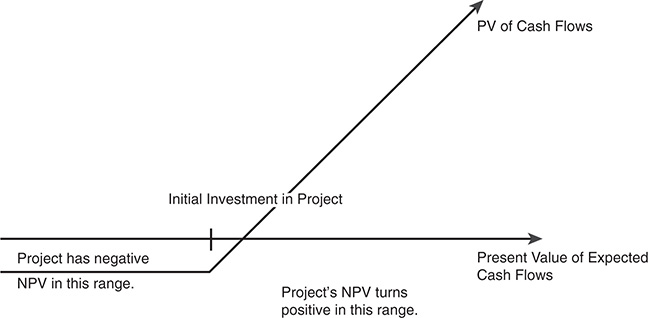
Note that this payoff diagram is that of a call option. The underlying asset is the investment. The option’s strike price is the initial outlay needed to initiate the investment. The option’s life is how long the firm has rights to the investment. The present value of the cash flows on this project and the expected variance in this present value represent the value and variance of the underlying asset.
Valuing an Option to Delay
On the surface, the inputs needed to apply option pricing theory to valuing the option to delay are the same as those needed for any option. We need the value of the underlying asset, the variance in that value, the time to expiration on the option, the strike price, the riskless rate, and the equivalent of the dividend yield (cost of delay). Actually estimating these inputs for product patent valuation can be difficult, however:
Value of the underlying asset: In this case, the underlying asset is the investment itself. The current value of this asset is the present value of expected cash flows from initiating the project now, not including the up-front investment, which can be obtained by doing a standard capital budgeting analysis. There is likely to be a substantial amount of error in the cash flow estimates and the present value, however. Rather than being viewed as a problem, this uncertainty should be viewed as the reason why the project delay option has value. If the expected cash flows on the project were known with certainty and were not expected to change, there would be no need to adopt an option pricing framework, because the option would have no value.
Variance in the value of the asset: The present value of the expected cash flows that measures the value of the asset will change over time. This is partly because the product’s potential market size might be unknown and partly because technological shifts can change the product’s cost structure and profitability. The variance in the present value of cash flows from the project can be estimated in one of three ways:
If similar projects have been introduced in the past, the variance in the cash flows from those projects can be used as an estimate. This might be how a consumer products company like Gillette might estimate the variance associated with introducing a new blade for its razors.
Probabilities can be assigned to various market scenarios, cash flows estimated under each scenario, and the variance estimated across present values. Alternatively, the probability distributions can be estimated for each of the inputs into the project analysis—the size of the market, the market share, and the profit margin, for instance—and simulations used to estimate the variance in the present values that emerge.
The variance in the market value of publicly traded firms involved in the same business (as the project being considered) can be used as an estimate of the variance. Thus, the average variance in firm value of firms involved in the software business can be used as the variance in present value of a software project.
The value of the option is largely derived from the variance in cash flows—the higher the variance, the higher the value of the project delay option. Thus, the value of an option to delay a project in a stable business will be less than the value of a similar option in an environment where technology, competition, and markets are all changing rapidly.
Exercise price on option: A project delay option is exercised when the firm owning the rights to the project decides to invest in it. The cost of making this investment is the option’s exercise price. The underlying assumption is that this cost remains constant (in present-value dollars) and that any uncertainty associated with the product is reflected in the present value of cash flows on the product.
Expiration of the option and the riskless rate: The project delay option expires when the rights to the project lapse. Investments made after the project rights expire are assumed to deliver a net present value of zero as competition drives returns down to the required rate. The riskless rate to use in pricing the option should be the rate that corresponds to the option’s expiration. Although the option life can be estimated easily when firms have explicit rights to a project (through a license or patent, for instance), obtaining it becomes far more difficult when firms have only a competitive advantage to take a project.
Cost of delay (dividend yield): There is a cost to delaying taking a project after the net present value turns positive. Because the project rights expire after a fixed period, and excess profits (which are the source of positive present value) are assumed to disappear after that time as new competitors emerge, each year of delay translates into one less year of value-creating cash flows.3 If the cash flows are evenly distributed over time, and the patent’s life is n years, the cost of delay can be written approximately as follows:
Thus, if the project rights are for 20 years, the annual cost of delay works out to 5% a year. Note, though, that this cost of delay rises each year, to 1/19 in year 2, 1/18 in year 3, and so on, making the cost-of-delay exercise larger over time. More generally, if the cash flows vary over time, the cost of delay can be written as follows:
Annual Cost of Delay = Expected CF next year/PV of cash flows on investment
Practical Considerations
While it is quite clear that the option to delay is embedded in many investments, several problems are associated with the use of option pricing models to value these options. First, the underlying asset in this option, which is the project, is not traded, which makes estimating its value and variance difficult. We would argue that the value can be estimated from the expected cash flows and the discount rate for the project, albeit with error. The variance is more difficult to estimate, however, because we are attempting to estimate a variance in project value over time.
Second, the behavior of prices over time might not conform to the price path assumed by the option pricing models. In particular, the assumption that values move in small increments continuously (an assumption of the Black-Scholes model), and that the variance in value remains unchanged over time, might be difficult to justify in the context of a real investment. For instance, a sudden technological change might dramatically change a project’s value, either positively or negatively.
Third, there might be no specific period for which the firm has rights to the project. For instance, a firm might have significant advantages over its competitors. This might, in turn, provide it with virtually exclusive rights to a project for a period of time. The rights are not legal restrictions, however, and they could erode faster than expected. In such cases, the expected life of the project itself is uncertain and is only an estimate. Ironically, uncertainty about the option’s expected life can increase the variance in present value, and through it, the expected value of the rights to the project.
Applications of the Option to Delay
The option to delay provides interesting perspectives on two common investment problems. The first is in the valuation of patents, especially those that are not viable today but could be viable in the future. By extension, this also allows us to look at whether R&D expenses deliver value. The second is in the analysis of natural resource assets such as vacant land and undeveloped oil reserves.
Patents
A product patent gives a firm the right to develop and market a product. But the firm will do so only if the present value of the expected cash flows from the product sales exceed the cost of development, as shown in Figure 5.4. If this does not occur, the firm can shelve the patent and not incur any further costs. If I is the present value of the costs of developing the product, and V is the present value of the expected cash flows from development, the payoffs from owning a product patent can be written as follows:
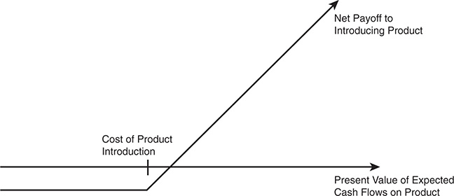
Thus, a product patent can be viewed as a call option, where the product itself is the underlying asset.4
The implications of viewing patents as options can be significant. First, it implies that nonviable patents will continue to have value, especially in businesses that have substantial volatility. Second, it indicates that firms might hold off on developing viable patents if they feel that they gain more from waiting than they lose in terms of cash flows. This behavior is more common if no significant competition is on the horizon. Third, the value of patents will be higher in risky businesses than in safe businesses, because option value increases with volatility. If we consider R&D to be the expense associated with acquiring these patents, this would imply that research should have its biggest payoff when directed to areas where less is known and more uncertainty exists. Consequently, we should expect pharmaceutical firms to spend more of their R&D budgets on gene therapy than on flu vaccines.5 We return to examine this issue in more depth in Chapter 15, “Invisible Investments: Valuing Firms with Intangible Assets.”
Natural Resource Options
In a natural resource investment, the underlying asset is the natural resource, and the asset’s value is based on two variables: the estimated quantity and the price of the resource. Thus, in a gold mine, for example, the value of the underlying asset is the value of the estimated gold reserves in the mine, based on the current price of gold. In most such investments, an initial cost is associated with developing the resource. The difference between the value of the asset extracted and the cost of the development is the profit to the owner of the resource (see Figure 5.5). Defining the cost of development as X, and the estimated value of the developed resource as V, the potential payoffs on a natural resource option can be written as follows:
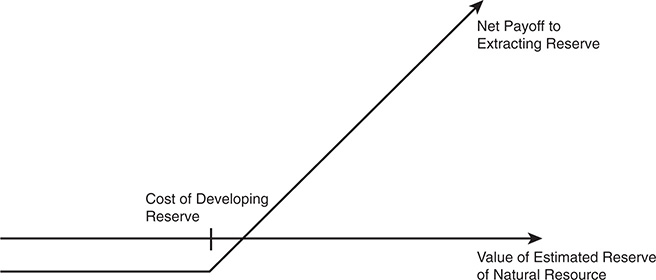
Thus, the investment in a natural resource option has a payoff function similar to a call option.6
What are the implications of viewing natural resource reserves as options? The first is that the value of a natural resource company can be written as a sum of two values: the conventional risk-adjusted value of expected cash flows from developed reserves, and the option value of undeveloped reserves. Although both will increase in value as the price of the natural resource increases, the latter will respond positively to increases in price volatility. Thus, the values of oil companies should increase if oil price volatility increases, even if oil prices themselves do not go up. The second implication is that conventional discounted cash flow valuation will understate the value of natural resource companies, even if the expected cash flows are unbiased and reasonable, because it will miss the option premium inherent in their undeveloped reserves. The third implication is that development of natural resource reserves will slow down as the volatility in prices increases. The time premium on the options will increase, making exercise of the options (development of the reserves) less likely. The same type of analysis can be extended to any other commodity company (gold and copper reserves, for instance) and even to vacant land or real estate properties. The owner of vacant land in Manhattan can choose whether and when to develop the land and will make that decision based on real estate values.7
Mining and commodity companies have been at the forefront of using real options in decision making. Their usage of the technology predates the current boom in real options. One reason is that natural resource options come closest to meeting the prerequisites for the use of option pricing models. Firms can learn a great deal by observing commodity prices and can adjust their behavior (in terms of development and exploration) quickly. In addition, if we consider exclusivity to be a prerequisite for real options to have value, that exclusivity for natural resource options derives from their natural scarcity. After all, only a finite amount of oil and gold is under the ground, and there’s only so much vacant land in Manhattan. Finally, natural resource reserves come closest to meeting the arbitrage/replication requirements that option pricing models are built on; both the underlying asset (the natural resource) and the option can often be bought and sold. We examine the use of real options models in commodity company valuations in more depth in Chapter 13, “Ups and Downs: Valuing Cyclical and Commodity Companies.”
The Option to Expand an Investment
In some cases, a firm takes an investment because doing so allows it either to make other investments or to enter other markets in the future. In such cases, it can be argued that the initial investment provides the firm with an option to expand, and the firm should therefore be willing to pay a price for such an option. Consequently, a firm might be willing to lose money on the first investment because it perceives the option to expand as having a large-enough value to compensate for the initial loss.
To examine this option, assume that the present value of the expected cash flows from entering the new market or taking the new project is V, and the total investment needed to enter this market or take this project is X. Furthermore, assume that the firm has a fixed time horizon, at the end of which it must decide whether to take advantage of this opportunity. Finally, assume that the firm cannot move forward on this opportunity if it does not take the initial investment. This scenario implies the option payoffs shown in Figure 5.6.
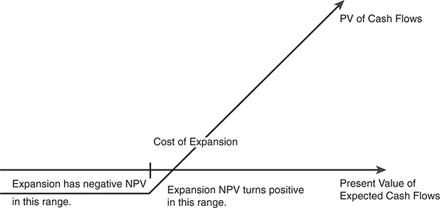
As you can see, at the expiration of the fixed time horizon, the firm enters the new market or takes the new investment if the present value of the expected cash flows at that point in time exceeds the cost of entering the market.
Consider a simple example of an option to expand. Disney is considering starting a Spanish version of the Disney Channel in Mexico. It estimates the investment will lose money and have a negative net present value. The negative net present value normally would suggest that rejecting the investment is the best course. However, assume that if the Mexican venture does better than expected, Disney plans to expand the network into the rest of Latin America at a significant cost. Based on its current assessment of this market, Disney believes that the present value of the expected cash flows on this investment will be less than the cost, yielding a negative net present value for that investment as well. The saving grace is that the latter present value is an estimate and Disney does not have a firm grasp of the market, and there is significant uncertainty about that value. Finally, assume that Disney will have to make this expansion decision within a fixed period (say, five years) of the Mexican investment.
We can value the Latin American expansion as an option, with the uncertainty about its value generating the value for the option. If the value of the expansion option is greater than the value lost on the initial investment in Mexico, Disney could justify the investment.
The practical considerations associated with estimating the value of the option to expand are similar to those associated with valuing the option to delay. In most cases, firms with options to expand have no specific time horizon by which they have to make an expansion decision, making these open-ended options or, at best, options with arbitrary lives. Even in cases where a life can be estimated for the option, neither the size nor the product’s potential market might be known, and estimating either can be problematic. To illustrate, consider again the Disney example. Although we adopted a period of five years, at the end of which Disney must decide on its future expansion into Latin America, it is entirely possible that this time frame is not specified when the channel goes on the air. Furthermore, we have assumed that both the cost and present value of expansion are known initially. In reality, the firm might not have good estimates for either before making the first investment, because it does not have much information on the underlying market.
Implications
The option to expand is implicitly used by firms to rationalize making investments that have negative net present value but that provide significant opportunities to tap into new markets or sell new products. The option pricing approach not only adds rigor to this argument by estimating the value of this option, it also provides insight into occasions when it is most valuable. In general, the option to expand is clearly more valuable for more volatile businesses with higher returns on projects (such as biotechnology or computer software) than for stable businesses with lower returns (such as housing, utilities, or automobile production). Specifically, the option to expand is at the basis of arguments that an investment should be made because of strategic considerations or that large investments should be broken into smaller phases. It can also be considered a rationale for why firms might accumulate cash or hold back on borrowing, thus preserving financial flexibility.
Strategic Considerations
In many acquisitions or investments, the acquiring firm believes that the transaction will give it competitive advantages in the future. These competitive advantages run the gamut:
Entry into a growing or large market: An investment or acquisition might allow the firm to enter a large or potentially large market much sooner than it otherwise would have been able to. An example of this is the acquisition of a Mexican retail firm by a U.S. firm, with the intent of expanding into the Mexican market.
Technological expertise: In some cases, the acquisition is motivated by the desire to acquire a proprietary technology that will allow the acquirer to either expand its existing market or expand into a new market.
Brand name: Firms sometimes pay large premiums over market price to acquire firms with valuable brand names, because they believe that these brand names can be used to expand into new markets in the future.
Although all these potential advantages may be used to justify initial investments that do not meet financial benchmarks, not all of them create valuable options. The value of the option is derived from the degree to which these competitive advantages, assuming that they do exist, translate into sustainable excess returns. As a consequence, these advantages can be used to justify premiums only in cases where the acquiring firm believes that it has some degree of exclusivity in the targeted market or technology. Two examples can help illustrate this point. A telecommunications firm should be willing to pay a premium for a Chinese telecomm firm if the latter has exclusive rights to service a large segment of the Chinese market. The option to expand into the Chinese market could be worth a significant amount.8 On the other hand, a developed market retailer should be wary about paying a real options premium for an Indian retail firm, even though it might believe that the Indian market could grow to be a lucrative one. The option to expand into this lucrative market is open to all entrants, not just existing retailers, so it might not translate into sustainable excess returns. Put simply, opportunities are not options.
Multistage Projects and Investments
When entering new businesses or making new investments, firms can sometimes do so in stages. Although doing so might reduce potential upsides, it also protects the firm from downside risk by allowing it, at each stage, to gauge demand and decide whether to go on to the next stage. In other words, a standard project can be recast as a series of options to expand, with each option being dependent on the previous one. Two propositions follow:
Some projects that do not look good on a full investment basis might be value-creating if the firm can invest in stages.
Some projects that look attractive on a full investment basis might become even more attractive if taken in stages.
The gain in value from the options created by multistage investments must be weighed against the cost. Taking investments in stages might allow competitors who decide to enter the market on a full scale to capture the market. It might also lead to higher costs at each stage, because the firm is not taking full advantage of economies of scale.
Several implications emerge from viewing this choice between multistage and one-time investments in an option framework. Here are some projects where the gains will be largest from making the investment in multiple stages:
Projects that have significant barriers to entry from competitors entering the market and taking advantage of delays in full-scale production. Thus, a firm with a patent on a product or other legal protection against competition pays a much smaller price for starting small and expanding as it learns more about the product.
Projects where there is significant uncertainty about the size of the market and the project’s eventual success: Here, starting small and expanding allows the firm to reduce its losses if the product does not sell as well as anticipated and to learn more about the market at each stage. This information can then be useful in subsequent stages in both product design and marketing. Hsu argues that venture capitalists invest in young companies in stages partly to capture the value option of waiting/learning at each stage and partly to reduce the likelihood that the entrepreneur will be too conservative in pursuing risky (but good) opportunities.9
Projects that need a substantial investment in infrastructure (large fixed costs) and high operating leverage: Because the savings from doing a project in multiple stages can be traced to investments needed at each stage, they are likely to be greater in firms where those costs are large. Capital-intensive projects as well as projects that require large initial marketing expenses (a new brand-name product for a consumer product company) will gain more from the options created by taking the project in multiple stages.
Growth Companies
In the stock market boom of the 1990s, we witnessed the phenomenon of young start-up dot com companies with large market capitalizations but little to show in terms of earnings, cash flows, or even revenues. Conventional valuation models suggested that justifying these market valuations with expected cash flows would be difficult, if not impossible. In an interesting twist on the option-to-expand argument, some people argued that investors in these companies were buying options to expand to be part of a potentially huge e-commerce market, rather than conventional stock.10
While the argument is alluring and serves to pacify investors in growth companies who might feel that they are paying too much, clearly dangers exist in making this stretch. The biggest one is that the “exclusivity” component that is necessary for real options to have value is being given short shrift. Suppose that you invested in a dot com stock in 1999, and assume that you were paying a premium to be part of a potentially large online market today. Assume further that this market comes to fruition. Could you have partaken in this market without paying that upfront premium for a dot-com company? We don’t see why not. After all, Walmart and Apple were just as capable of being part of this online market as were any number of new entrants into the market.
Financial Flexibility
When making decisions about how much to borrow and how much cash to return to stockholders (in dividends and stock buybacks), managers should consider the effects that such decisions will have on their capacity to make new investments or meet unanticipated contingencies in the future. Practically, this translates into firms maintaining excess debt capacity or larger cash balances than are warranted by current needs to meet unexpected future requirements. While maintaining this financing flexibility has value for firms, it also has costs. The large cash balances might earn below-market returns, and excess debt capacity implies that the firm is giving up some value by maintaining a higher cost of capital.
Using an option framework, it can be argued that a firm that maintains a large cash balance and preserves excess debt capacity does so to have the option to take unexpected projects with high returns that might arise in the future. To value financial flexibility as an option, consider the following framework: A firm has expectations about how much it will need to reinvest in future periods, based on its own history and current conditions in the industry. On the other side of the ledger, a firm also has expectations about how much it can raise from internal funds and its normal access to capital markets in the future. Assume that actual reinvestment needs can be very different from the expected reinvestment needs. For simplicity, we will assume that the firm knows its capacity to generate funds. The advantage (and value) of having excess debt capacity or large cash balances is that the firm can meet any reinvestment needs in excess of funds available using its excess debt capacity and surplus cash. The payoff from these projects, however, comes from the excess returns that the firm expects to make on them.
Looking at financial flexibility as an option yields valuable insights into when financial flexibility is most valuable. Using the framework we just developed, for instance, we would argue the following:
Other things remaining equal, firms operating in businesses where projects earn substantially higher returns than their hurdle rates should value flexibility more than those that operate in stable businesses where excess returns are small. This would imply that firms that earn large excess returns on their projects can use the need for financial flexibility as the justification for holding large cash balances and excess debt capacity.
Because a firm’s ability to fund these reinvestment needs is determined by its capacity to generate internal funds, other things remaining equal, financial flexibility should be worth less to firms with large and stable earnings as a percent of firm value. Young and growing firms that have small or negative earnings, and therefore much lower capacity to generate internal funds, will value flexibility more. As supporting evidence, note that technology firms usually borrow very little and accumulate large cash balances.
Firms with limited internal funds can still get away with little or no financial flexibility if they can tap external markets for capital—bank debt, bonds, and new equity issues. Other things remaining equal, the greater a firm’s capacity (and willingness) to raise funds from external capital markets, the less should be the value of flexibility. This might explain why private or small firms, which have far less access to capital, value financial flexibility more than larger firms. The existence of corporate bond markets can also make a difference in how much flexibility is valued. In markets where firms cannot issue bonds and have to depend entirely on banks for financing, there is less access to capital and a greater need to maintain financial flexibility.
The need for and value of flexibility is a function of how uncertain a firm is about future reinvestment needs. Firms with predictable reinvestment needs should value flexibility less than firms in sectors where reinvestment needs are volatile on a period-to-period basis.
In conventional corporate finance, the optimal debt ratio is the one that minimizes the cost of capital. Little incentive exists for firms to accumulate cash balances. This view of the world, though, flows directly from the implicit assumption we make that capital markets are open and can be accessed with little or no cost. Introducing capital constraints, internal or external, into the model leads to a more nuanced analysis where rational firms might borrow less than optimal and hold back on returning cash to stockholders.
The Option to Abandon an Investment
The final option to consider is the option to abandon a project when its cash flows do not measure up to expectations. One way to reflect this value is through decision trees, as discussed in Chapter 3. The decision tree has limited applicability in most real-world investment analyses; it typically works only for multistage projects, and it requires inputs on probabilities at each stage of the project. The option pricing approach provides a more general way of estimating and building the value of abandonment into investment analysis. To illustrate, assume that V is the remaining value on a project if it continues to the end of its life, and L is the liquidation or abandonment value for the same project at the same point in time. If the project has a life of n years, the value of continuing the project can be compared to the liquidation (abandonment) value. If the value from continuing is higher, the project should be continued; if the value of abandonment is higher, the holder of the abandonment option could consider abandoning the project:
If V > L: Continue with the project
If V < L: Abandon project and receive L-V
These payoffs are graphed in Figure 5.7 as a function of the expected value from continuing the investment.
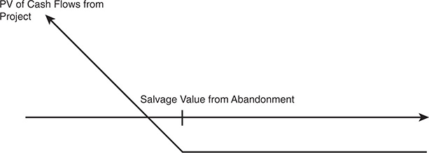
Unlike the options to delay and expand, the option to abandon takes on the characteristics of a put option.
Consider a simple example. Assume that a firm is considering taking a ten-year project that requires an initial investment of $100 million in a real estate partnership, where the present value of expected cash flows is $90 million. While the net present value is negative (−$10 million), assume that the firm has the option to abandon this project anytime in the next ten years by selling its share of the ownership to the other partners in the venture for $50 million.
If the value of this abandonment option is greater than $10 million (which is the negative net present value of the investment), the investment makes sense. Note, though, that abandonment becomes a more and more attractive option as the remaining project life decreases, because the present value of the remaining cash flows decreases.
In the preceding analysis, we assumed, rather unrealistically, that the abandonment value was clearly specified up front and that it did not change during the life of the project. This might be true in some very specific cases, in which an abandonment option is built into the contract. More often, however, the firm has the option to abandon, and the salvage value from doing so has to be estimated (with error) up front. Further, the abandonment value might change over the life of the project, making it difficult to apply traditional option pricing techniques. Finally, it is entirely possible that abandoning a project might not bring in a liquidation value, but might create costs instead. A manufacturing firm might have to pay severance to its workers, for instance. In such cases, abandoning would not make sense, unless the present value of the expected cash flows from continuing with the investment are even more negative.
Implications
The fact that the option to abandon has value provides a rationale for firms to build in operating flexibility to scale back or terminate projects if they do not measure up to expectations. It also indicates that firms that focus on generating more revenues by offering their customers the option to walk away from commitments might be giving up more than they gain.
Escape Clauses
When a firm enters into a long-term risky investment that requires a large up-front investment, it should do so with the clear understanding that it might regret making this investment fairly early in its life. Being able to get out of such long-term commitments that threaten to drain more resources in the future is at the heart of the option to abandon. It is true that some of this flexibility is determined by the business you are in; getting out of bad investments is easier to do in service businesses than in heavy infrastructure businesses. However, it is also true that firms can take actions at the time of making these investments that give them more choices if things do not go according to plan.
The first and most direct way is to build operating flexibility contractually with the parties that are involved in the investment. Thus, contracts with suppliers may be written on an annual basis rather than long-term, and employees may be hired on a temporary basis rather than permanently. The physical plant used for a project may be leased on a short-term basis rather than bought, and the financial investment may be made in stages rather than as an initial lump sum. Although there is a cost to building in this flexibility, the gains might be much larger, especially in volatile businesses. The initial capital investment can be shared with another investor, presumably with deeper pockets and a greater willingness to stay with the investment, even if it turns sour. This provides a rationale for joint venture investing, especially for small firms that have limited resources; finding a cash-rich, larger company to share the risk might well be worth the cost.
None of these actions is costless. Entering into short-term agreements with suppliers and leasing the physical plant might be more expensive than committing for the life of the investment, but that additional cost has to be weighed against the benefit of maintaining the abandonment option.
Customer Incentives
Firms that are intent on increasing revenues sometimes offer customers abandonment options to induce them to buy their products and services. Consider a firm that sells its products on multiyear contracts and that offers customers the option to cancel their contracts at any time, with no cost. Even though this might sweeten the deal and increase sales, a substantial cost is likely. In the event of a recession, customers who are unable to meet their obligations are likely to cancel their contracts. In effect, the firm has made its good times better and its bad times worse. The cost of this increased volatility in earnings and revenues has to be measured against the potential gain in revenue growth to see whether the net effect is positive.
This discussion should also be a cautionary note for firms that are run with marketing objectives such as maximizing market share or posting high-revenue growth. Those objectives can often be accomplished by giving customers valuable options. Salespeople want to meet their sales targets and are not particularly concerned about the long-term costs they might create with their commitments to customers—and the firm might be worse off as a consequence.
Switching Options
Although the abandonment option considers the value of shutting down an investment, an intermediate alternative is worth examining. Firms can sometimes alter production levels in response to demand. Being able to do so can make an investment more valuable. Consider, for instance, a power company that is considering a new plant to generate electricity. Assume that the company can run the plant at full capacity and produce 1 million kilowatt-hours of power or run it at half capacity (and substantially less cost) and produce 500,000 kilowatt-hours of power. In this case, the company can observe both the demand for power and the revenues per kilowatt-hour and decide whether it makes sense to run at full or half capacity. The value of this switching option can then be compared to the cost of building in this flexibility in the first place.
The airline business provides an interesting case study in how different companies manage their cost structure and the payoffs to their strategies. One reason that Southwest Airlines has been able to maintain its profitability in a deeply troubled sector is that the company has made cost flexibility a central component of its decision process. From its initial choice of using only one type of aircraft for its entire fleet11 to its refusal, for the most part, to fly into large urban airports (with high gate costs), the company’s operations have created the most flexible cost structure in the business. Thus, when revenues dip (as they inevitably do when the economy weakens), Southwest can trim its costs and stay profitable while other airlines teeter on the brink of bankruptcy.
Caveats for Real Options
The discussion of the potential applications of real options should provide a window into why they are so alluring to practitioners and businesses. In essence, we are ignoring the time-honored rules of capital budgeting, which include rejecting investments that have negative net present value, when real options are present. Not only does the real options approach encourage you to make investments that do not meet conventional financial criteria, it also makes it more likely that you will do so the less you know about the investment. Ignorance, rather than being a weakness, becomes a virtue, because it increases the uncertainty in the estimated value and the resulting option value. To prevent the real options process from being hijacked by managers who want to rationalize bad (and risky) decisions, we have to impose some reasonable constraints on when it can be used. And when it is used, we have to specify how to estimate its value.
First, not all investments have options embedded in them, and not all options, even if they do exist, have value. To assess whether an investment creates valuable options that need to be analyzed and valued, three key questions need to be answered affirmatively:
Is the first investment a prerequisite for the later investment/expansion? If not, how necessary is the first investment for the later investment/expansion? Consider our earlier analysis of the value of a patent or the value of an undeveloped oil reserve as options. A firm cannot generate patents without investing in research or paying another firm for the patents, and it cannot get rights to an undeveloped oil reserve without bidding on it at a government auction or buying it from another oil company. Clearly, the initial investment here (spending on R&D, bidding at the auction) is required for the firm to have the second option. Now consider the Disney expansion into Mexico. The initial investment in a Spanish channel provides Disney with information about market potential, without which presumably it is unwilling to expand into the larger Latin American market. Unlike the examples of patents and undeveloped reserves, the initial investment is not a prerequisite for the second, although management might view it as such. The connection gets even weaker when we look at one firm acquiring another to have the option to be able to enter a large market. Acquiring an Internet service provider to have a foothold in the Internet retailing market or buying a Brazilian brewery to preserve the option to enter the Brazilian beer market are examples of such transactions.
Does the firm have an exclusive right to the later investment/expansion? If not, does the initial investment provide the firm with significant competitive advantages on subsequent investments? The value of the option ultimately derives not from the cash flows generated by the second and subsequent investments, but from the excess returns generated by these cash flows. The greater the potential for excess returns on the second investment, the greater the value of the option in the first investment. The potential for excess returns is closely tied to how much of a competitive advantage the first investment provides the firm when it takes subsequent investments. At one extreme, again, consider investing in research and development to acquire a patent. The patent gives the firm that owns it the exclusive rights to produce that product and, if the market potential is large, the right to the excess returns from the project. At the other extreme, the firm might get no competitive advantages on subsequent investments. In that case, whether these investments can generate any excess returns is questionable. In reality, most investments fall in between these two extremes, with greater competitive advantages being associated with higher excess returns and larger option values.
How sustainable are the competitive advantages? In a competitive marketplace, excess returns attract competitors, and competition drives out excess returns. The more sustainable the competitive advantages possessed by a firm, the greater the value of the options embedded in the initial investment. The sustainability of competitive advantages is a function of two forces. The first is the nature of the competition; other things remaining equal, competitive advantages fade much more quickly in sectors that have aggressive competitors, and new entry into the business is easy. The second is the nature of the competitive advantage. If the resource controlled by the firm is finite and scarce (as is the case with natural resource reserves and vacant land), the competitive advantage is likely to be sustainable for longer periods. Alternatively, if the competitive advantage comes from being the first mover in a market or technological expertise, it will come under assault far sooner. The most direct way of reflecting this in the value of the option is in its life. The option’s life can be set to the period of competitive advantage. Only the excess returns earned over this period count toward the value of the option.
Second, when real options are used to justify a decision, the justification has to be in more than qualitative terms. In other words, managers who argue for taking a project with poor returns or for paying a premium on an acquisition on the basis of real options should be required to value these real options. They also should be required to show that the economic benefits exceed the costs. Two arguments can be made against this requirement. The first is that real options cannot be easily valued, because the inputs are difficult to obtain and often noisy. The second is that the inputs to option pricing models can be easily manipulated to back up whatever the conclusion might be. Although both arguments have some basis, an estimate with error is better than no estimate at all. The process of quantitatively trying to estimate the value of a real option is, in fact, the first step to understanding what drives its value.
We should mention a final note of caution about the use of option pricing models to assess the value of real options. Option pricing models, whether they are of the binomial or Black Scholes variety, are based on two fundamental precepts—replication and arbitrage. For either to be feasible, you have to be able to trade on the underlying asset and on the option. This is easy to accomplish with a listed option on a traded stock; you can trade on both the stock and the listed option. It is much more difficult to pull off when valuing a patent or an investment expansion opportunity. Neither the underlying asset (the product that emerges from the patent) nor the option itself is traded. This does not mean that you cannot estimate the value of a patent as an option, but it does indicate that monetizing this value will be much more difficult. Much as you might believe in option model value as the right estimate of value, it is unlikely that any potential buyer of the patent will come close to paying that amount.
Conclusion
In contrast to the approaches that focus on downside risk—risk-adjusted value, simulations, and decision trees—the real options approach brings an optimistic view to uncertainty. While conceding that uncertainty can create losses, it argues that uncertainty can also be exploited for potential gains and that updated information can be used to augment the upside and reduce the downside risks inherent in investments. In essence, you are arguing that the conventional risk-adjustment approaches fail to capture this flexibility and that you should add an option premium to the risk-adjusted value.
This chapter considered three potential real options and applications of each. The first is the option to delay. This is where a firm with exclusive rights to an investment has the option of deciding when to take that investment and to delay taking it, if necessary. The second is the option to expand. This is where a firm might be willing to lose money on an initial investment in the hopes of expanding into other investments or markets further down the road. The third is the option to abandon an investment if it looks like a money loser, early in the process.
Although it is clearly appropriate to attach value to real options in some cases—patents, reserves of natural resources, or exclusive licenses—the argument for an option premium gets progressively weaker as we move away from the exclusivity inherent in each of these cases. In particular, a firm that invests in an emerging market in a money-losing enterprise, using the argument that the market is a large and potentially profitable one, could be making a serious mistake. After all, the firm could be right in its assessment of the market, but absent barriers to entry, it might not be able to earn excess returns in that market or keep out the competition. Not all opportunities are options, and not all options have significant economic value.
Appendix: Basics of Options and Option Pricing
An option provides the holder with the right to buy or sell a specified quantity of an underlying asset at a fixed price (called a strike price or an exercise price) at or before the expiration date of the option. Because it is a right and not an obligation, the holder can choose not to exercise the right and allow the option to expire. The two types of options are call options and put options.
Option Payoffs
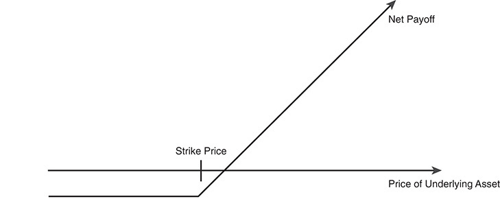
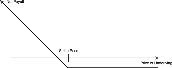
A call option gives the option buyer the right to buy the underlying asset at a fixed price, called the strike or the exercise price, at any time prior to the expiration date of the option: the buyer pays a price for this right. If at expiration the value of the asset is less than the strike price, the option is not exercised and expires worthless. If, on the other hand, the value of the asset is greater than the strike price, the option is exercised—the option buyer buys the stock at the exercise price and the difference between the asset value and the exercise price comprises the gross profit on the investment. The net profit on the investment is the difference between the gross profit and the price paid for the call initially. A payoff diagram illustrates the cash payoff on an option at expiration. For a call, the net payoff is negative (and equal to the price paid for the call) if the value of the underlying asset is less than the strike price. If the price of the underlying asset exceeds the strike price, the gross payoff is the difference between the value of the underlying asset and the strike price, and the net payoff is the difference between the gross payoff and the price of the call. This is illustrated in the Figure 5A.1.
A put option gives the option buyer the right to sell the underlying asset at a fixed price, again called the strike or exercise price, any time prior to the expiration date of the option. The buyer pays a price for this right. If the price of the underlying asset is greater than the strike price, the option will not be exercised and will expire worthless. If on the other hand, the price of the underlying asset is less than the strike price, the owner of the put option will exercise the option and sell the stock at the strike price, claiming the difference between the strike price and the market value of the asset as the gross profit. Again, netting out the initial cost paid for the put yields the net profit from the transaction. A put has a negative net payoff if the value of the underlying asset exceeds the strike price and has a gross payoff equal to the difference between the strike price and the value of the underlying asset if the asset value is less than the strike price. This is summarized in Figure 5A.2.
One final distinction needs to be made. Options are usually categorized as American or European options. A primary distinction between the two is that American options can be exercised at any time prior to their expiration, whereas European options can be exercised only at expiration. The possibility of early exercise makes American options more valuable than otherwise similar European options; it also makes them more difficult to value. One compensating factor exists that enables the former to be valued using models designed for the latter. In most cases, the time premium associated with the remaining life of an option and transactions costs makes early exercise suboptimal. In other words, the holders of in-the-money options will generally get much more by selling the option to someone else than by exercising the options.1
Determinants of Option Value
The value of an option is determined by a number of variables relating to the underlying asset and financial markets.
Current value of the underlying asset: Options are assets that derive value from an underlying asset. Consequently, changes in the value of the underlying asset affect the value of the options on that asset. Because calls provide the right to buy the underlying asset at a fixed price, an increase in the value of the asset will increase the value of the calls. Puts, on the other hand, become less valuable as the value of the asset increase.
Variance in value of the underlying asset: The buyer of an option acquires the right to buy or sell the underlying asset at a fixed price. The higher the variance in the value of the underlying asset, the greater the value of the option. This is true for both calls and puts. Although it might seem counterintuitive that an increase in a risk measure (variance) should increase value, options are different from other securities because buyers of options can never lose more than the price they pay for them; in fact, they have the potential to earn significant returns from large price movements.
Dividends paid on the underlying asset: We can expect the value of the underlying asset to decrease if dividend payments are made on the asset during the life of the option. Consequently, the value of a call on the asset is a decreasing function of the size of expected dividend payments, and the value of a put is an increasing function of expected dividend payments. A more intuitive way of thinking about dividend payments, for call options, is as a cost of delaying exercise on in-the-money options. To see why, consider an option on a traded stock. When a call option is in the money, that is, the holder of the option will make a gross payoff by exercising the option, exercising the call option will provide the holder with the stock and entitle him or her to the dividends on the stock in subsequent periods. Failing to exercise the option means that these dividends are foregone.
Strike price of option: A key characteristic used to describe an option is the strike price. In the case of calls, where the holder acquires the right to buy at a fixed price, the value of the call declines as the strike price increases. In the case of puts, where the holder has the right to sell at a fixed price, the value increases as the strike price increases.
Time to expiration on option: Both calls and puts become more valuable as the time to expiration increases. This is because the longer time to expiration provides more time for the value of the underlying asset to move, increasing the value of both types of options. Additionally, in the case of a call, where the buyer has to pay a fixed price at expiration, the present value of this fixed price decreases as the life of the option increases, increasing the value of the call.
Riskless interest rate corresponding to life of option: Because the buyer of an option pays the price of the option up front, an opportunity cost is involved. This cost depends on the level of interest rates and the time to expiration on the option. The riskless interest rate also enters into the valuation of options when the present value of the exercise price is calculated because the exercise price does not have to be paid (received) until expiration on calls (puts). Increases in the interest rate increase the value of calls and reduce the value of puts.
Table 5A.1 summarizes the variables and their predicted effects on call and put prices.
Table 5A.1 Summary of Variables Affecting Call and Put Prices
|
Effect on |
|
Factor |
Call Value |
Put Value |
Increase in underlying asset’s value |
Increases |
Decreases |
Increase in strike price |
Decreases |
Increases |
Increase in variance of underlying asset |
Increases |
Increases |
Increase in time to expiration |
Increases |
Increases |
Increase in interest rates |
Increases |
Decreases |
Increase in dividends paid |
Decreases |
Increases |
Option Pricing Models
Option pricing theory has made vast strides since 1972, when Black and Scholes published their path-breaking paper providing a model for valuing dividend-protected European options. Black and Scholes used a “replicating portfolio”—a portfolio composed of the underlying asset and the risk-free asset that had the same cash flows as the option being valued—to derive their final formulation. Although their derivation is mathematically complicated, there is a simpler binomial model for valuing options that draws on the same logic.
The Binomial Model
The binomial option pricing model is based on a simple formulation for the asset price process, in which the asset can move to one of two possible prices in any time period. The general formulation of a stock price process that follows the binomial is shown in Figure 5A.3.
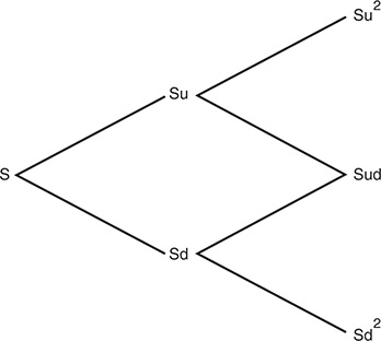
In this figure, S is the current stock price; the price moves up to Su with probability p and down to Sd with probability 1−p in any time period.
The objective in creating a replicating portfolio is to use a combination of risk-free borrowing/lending and the underlying asset to create the same cash flows as the option being valued. The principles of arbitrage apply here, and the value of the option must be equal to the value of the replicating portfolio. In the case of the preceding general formulation, where stock prices can either move up to Su or down to Sd in any time period, the replicating portfolio for a call with strike price K involves borrowing $B and acquiring ∆ of the underlying asset, where:
∆ = Number of Units of the Underlying Asset Bought = (Cu − Cd)/(Su − Sd)
where
Cu = Value of the Call If the Stock Price Is Su
Cd = Value of the Call If the Stock Price Is Sd
In a multiperiod binomial process, the valuation has to proceed iteratively; that is, starting with the last time period and moving backward in time until the current point in time. The portfolios replicating the option are created at each step and valued, providing the values for the option in that time period. The final output from the binomial option pricing model is a statement of the value of the option in terms of the replicating portfolio, composed of ∆ shares (option delta) of the underlying asset and risk-free borrowing/lending:
Value of the Call = Current Value of Underlying Asset × Option Delta − Borrowing Needed to Replicate the Option
Consider a simple example (see Figure 5A.4). Assume that the objective is to value a call with a strike price of 50, which is expected to expire in 2 time periods, on an underlying asset whose price currently is 50 and is expected to follow a binomial process:
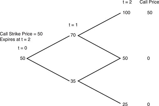
Now assume that the interest rate is 11%. In addition, define
∆ = Number of Shares in the Replicating Portfolio
B = Dollars of Borrowing in Replicating Portfolio
The objective is to combine ∆ shares of stock and B dollars of borrowing to replicate the cash flows from the call with a strike price of $50. This can be done iteratively, starting with the last period and working back through the binomial tree.
Step 1: Start with the end nodes and work backwards, as in Figure 5A.5
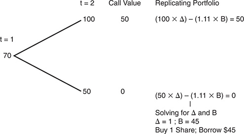
Thus, if the stock price is $70 at t = 1, borrowing $45 and buying 1 share of the stock will give the same cash flows as buying the call. The value of the call at t = 1, if the stock price is $70, is therefore:
Value of Call = Value of Replicating Position = 70 ∆ − B = 70 − 45 = 25
Considering the other leg of the binomial tree at t = 1, as in Figure 5A.6
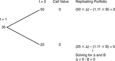
If the stock price is 35 at t = 1, then the call is worth nothing.
Step 2: Move backwards to the earlier time period and create a replicating portfolio that will provide the cash flows the option will provide (see Figure 5A.7).
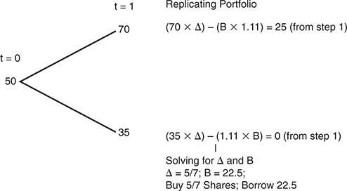
In other words, borrowing $22.50 and buying 5/7 of a share will provide the same cash flows as a call with a strike price of $50. The value of the call therefore has to be the same as the value of this position:
The binomial model provides insight into the determinants of option value. The value of an option is not determined by the expected price of the asset but by its current price, which, of course, reflects expectations about the future. This is a direct consequence of arbitrage. If the option value deviates from the value of the replicating portfolio, investors can create an arbitrage position, that is, one that requires no investment, involves no risk, and delivers positive returns. To illustrate, if the portfolio that replicates the call costs more than the call does in the market, an investor could buy the call, sell the replicating portfolio, and be guaranteed the difference as a profit. The cash flows on the two positions offset each other, leading to no cash flows in subsequent periods. The option value also increases as the time to expiration is extended, as the price movements (u and d) increase, and with increases in the interest rate.
The Black-Scholes Model
The binomial model is a discrete-time model for asset price movements, including a time interval (t) between price movements. As the time interval is shortened, the limiting distribution, as t approaches 0, can take one of two forms. If, as t approaches 0, price changes become smaller, the limiting distribution is the normal distribution and the price process is a continuous one. If, as t approaches 0, price changes remain large, the limiting distribution is the Poisson distribution, that is, a distribution that allows for price jumps. The Black-Scholes model applies when the limiting distribution is the normal distribution,2 and it explicitly assumes that the price process is continuous.
The Model
The original Black-Scholes model was designed to value European options, which were dividend-protected. Thus, neither the possibility of early exercise nor the payment of dividends affects the value of options in this model. The value of a call option in the Black-Scholes model can be written as a function of the following variables:
S = Current Value of the Underlying Asset
K = Strike Price of the Option
t = Life to Expiration of the Option
r = Riskless Interest Rate Corresponding to the Life of the Option
σ2 = Variance in the ln(Value) of the Underlying Asset
The model itself can be written as:
Value of Call = S N (d1) − K e−rt N(d2)
where
The process of valuation of options using the Black-Scholes model involves the following steps:
Step 1: The inputs to the Black-Scholes are used to estimate d1 and d2.
Step 2: The cumulative normal distribution functions, N(d1) and N(d2), corresponding to these standardized normal variables are estimated.
Step 3: The present value of the exercise price is estimated, using the continuous time version of the present value formulation:
Present Value of Exercise Price = K e−rt
Step 4: The value of the call is estimated from the Black-Scholes model.
The determinants of value in the Black-Scholes are the same as those in the binomial—the current value of the stock price, the variability in stock prices, the time to expiration on the option, the strike price, and the riskless interest rate. The principle of replicating portfolios that is used in binomial valuation also underlies the Black-Scholes model. In fact, embedded in the Black-Scholes model is the replicating portfolio:
N(d1), which is the number of shares that are needed to create the replicating portfolio is called the option delta. This replicating portfolio is self-financing and has the same value as the call at every stage of the option’s life.
Model Limitations and Fixes
The version of the Black-Scholes model presented above does not take into account the possibility of early exercise or the payment of dividends, both of which impact the value of options. Adjustments exist, which although not perfect, provide partial corrections to value.
Dividends
The payment of dividends reduces the stock price. Consequently, call options become less valuable and put options more valuable as dividend payments increase. One approach to dealing with dividends is to estimate the present value of expected dividends paid by the underlying asset during the option life and subtract it from the current value of the asset to use as S in the model. Because this becomes impractical as the option life becomes longer, we would suggest an alternate approach. If the dividend yield (y = Dividends/Current Value of the Asset) of the underlying asset is expected to remain unchanged during the life of the option, the Black-Scholes model can be modified to take dividends into account:
C = S e−yt N(d1) − K e−rt N(d2)
where
From an intuitive standpoint, the adjustments have two effects. First, the value of the asset is discounted back to the present at the dividend yield to take into account the expected drop in value from dividend payments. Second, the interest rate is offset by the dividend yield to reflect the lower carrying cost from holding the stock (in the replicating portfolio). The net effect is a reduction in the value of calls, with the adjustment, and an increase in the value of puts.
Early Exercise
The Black-Scholes model is designed to value European options, whereas most options that we consider are American options, which can be exercised any time before expiration. Without working through the mechanics of valuation models, an American option should always be worth at least as much and generally more than a European option because of the early exercise option. Three basic approaches exist for dealing with the possibility of early exercise. The first is to continue to use the unadjusted Black-Scholes and regard the resulting value as a floor or conservative estimate of the true value. The second approach is to value the option to each potential exercise date. With options on stocks, this basically requires that we value options to each ex-dividend day and choose the maximum of the estimated call values. The third approach is to use a modified version of the binomial model to consider the possibility of early exercise.
Although estimating the prices for each node of a binomial is difficult, variances estimated from historical data can be used to compute the expected up and down movements in the binomial. To illustrate, if σ2 is the variance in ln(stock prices), the up and down movements in the binomial can be estimated as follows:
where u and d are the up and down movements per unit time for the binomial, T is the life of the option, and m is the number of periods within that lifetime. Multiplying the stock price at each stage by u and d yields the up and the down prices. These can then be used to value the asset.
The Impact of Exercise on the Value of The Underlying Asset
The derivation of the Black-Scholes model is based on the assumption that exercising an option does not affect the value of the underlying asset. This might be true for listed options on stocks, but it is not true for some types of options. For instance, the exercise of warrants increases the number of shares outstanding and brings fresh cash into the firm, both of which affect the stock price.3 The expected negative impact (dilution) of exercise decreases the value of warrants compared to otherwise similar call options. The adjustment for dilution in the Black-Scholes to the stock price is fairly simple. The stock price is adjusted for the expected dilution from the exercise of the options. In the case of warrants, for instance:
Dilution-Adjusted S = (S ns + W nw)/(ns + nw)
where
S = Current Value of the Stock
W = Market Value of Warrants Outstanding
nw = Number of Warrants Outstanding
ns = Number of Shares Outstanding
When the warrants are exercised, the number of shares outstanding increases, reducing the stock price. The numerator reflects the market value of equity, including both stocks and warrants outstanding. The reduction in S reduces the value of the call option.
An element of circularity exists in this analysis because the value of the warrant is needed to estimate the dilution-adjusted S, and the dilution-adjusted S is needed to estimate the value of the warrant. This problem can be resolved by starting off the process with an estimated value of the warrant (say, the exercise value) and then iterating with the new estimated value for the warrant until there is convergence.
Valuing Puts
The value of a put can be derived from the value of a call with the same strike price and the same expiration date through an arbitrage relationship that specifies that:
C − P = S − K e−rt
where C is the value of the call and P is the value of the put (with the same life and exercise price).
This arbitrage relationship can be derived fairly easily and is called put-call parity. To see why put-call parity holds, consider creating the following portfolio:
(a) Sell a call and buy a put with exercise price K and the same expiration date “t”
(b) Buy the stock at current stock price S
The payoff from this position is riskless and always yields K at expiration (t). To see this, assume that the stock price at expiration is S*:
Position |
Payoffs at t if S*>K |
Payoffs at t if S*<K |
Sell call |
−(S* − K) |
0 |
Buy put |
0 |
K − S* |
Buy stock |
S* |
S* |
Total |
K |
K |
Because this position yields K with certainty, its value must be equal to the present value of K at the riskless rate (K e-rt):
This relationship can be used to value puts. Substituting the Black-Scholes formulation for the value of an equivalent call,
Value of Put = S e−yt (N(d1) − 1) − K e−rt (N(d2) − 1)
where
___________________________
1. Copeland, T. E. and V. Antikarov, 2003, Real Options: A Practitioner’s Guide, Texere. For an alternate path to the same conclusion, see Brandao, L. E., J. S. Dyer, and W. J. Huhn, 2005, “Using Binomial Decision Trees to Solve Real-Option Valuation Problems,” Decision Analysis, v2, 69–88. They use the risk-neutral probabilities from the option pricing model in the decision tree to solve for the option’s value.
2. McDonald, R. and D. Siegel, 2002, “The Value of Waiting to Invest,” Quarterly Journal of Economics, v101, 707–728.
3. A value-creating cash flow is one that adds to the net present value because it is in excess of the required return for investments of equivalent risk.
4. Schwartz, E., 2002, “Patents and R&D as Real Options,” working paper, Anderson School at UCLA.
5. Pakes, A., 1986, “Patents as Options: Some Estimates of the Value of Holding European Patent Stocks,” Econometrica, v54, 755–784. Although this paper does not explicitly value patents as options, it examines the returns investors would have earned investing in companies that derive their value from patents. The return distribution resembles that of a portfolio of options, with most investments losing money but the winners providing disproportionate gains.
6. Brennan, M. and E. Schwartz, 1985, “Evaluating Natural Resource Investments,” The Journal of Business, v58, 135–157.
7. Quigg, L, 1993, “Empirical Testing of Real Option-Pricing Models,” Journal of Finance, vol. 48, 621–640. The author examined transaction data on 2,700 undeveloped and 3,200 developed real estate properties between 1976 and 1979 and found evidence of a premium arising from the option to wait in the former.
8. A note of caution needs to be added here. If the exclusive rights to a market come with no pricing power—in other words, the government sets the price you charge your customers—it might very well translate into zero excess returns (and no option value).
9. Hsu, Y., 2002, “Staging of Venture Capital Investment: A Real Options Analysis,” working paper, University of Cambridge.
10. Schwartz, E. S. and M. Moon, 2001, “Rational Pricing of Internet Companies Revisited,” The Financial Review 36, pp. 7–26. A simpler version of the same argument was made in Mauboussin, M., 1998, “Get Real: Using Real Options in Security Analysis,” CSFB Publication, June 23, 1999.
11. From its inception until recently, Southwest used the Boeing 737 as its workhorse, thus reducing the need to keep different maintenance crews at each airport it flies into.
1. Although early exercise is not optimal generally, there are at least two exceptions to this rule. One is a case in which the underlying asset pays large dividends, thus reducing the value of the asset and any call options on that asset. In this case, call options may be exercised just before an ex-dividend date, if the time premium on the options is less than the expected decline in asset value as a consequence of the dividend payment. The other exception arises when an investor holds both the underlying asset and deep in-the-money puts on that asset at a time when interest rates are high. In this case, the time premium on the put might be less than the potential gain from exercising the put early and earning interest on the exercise price.
2. Stock prices cannot drop below zero because of the limited liability of stockholders in publicly listed firms. Hence, stock prices by themselves cannot be normally distributed because a normal distribution requires some probability of infinitely negative values. The distribution of the natural logs of stock prices is assumed to be log-normal in the Black-Scholes model. This is why the variance used in this model is the variance in the log of stock prices.
3. Warrants are call options issued by firms, either as part of management compensation contracts or to raise equity.