
Chapter 14
Sample user-defined functions
In this chapter, you will:
Learn how to create and share user-defined functions
Review useful custom functions
Learn how to create and share
LAMBDAfunctions
Excel provides many built-in functions. However, sometimes you need a complex custom function that Excel doesn’t offer, such as a function that sums a range of cells based on their interior color.
So, what do you do? You could use the calculator next to you as you work your way down your list—but be careful not to enter the same number twice! Or, you could convert the data set to a table, set a SUBTOTAL function for visible cells in the total row, and filter by color. Both methods are time-consuming and prone to accidents. What to do?
You could write a procedure to solve this problem—after all, that’s what this book is about. However, you have other options: user-defined functions (UDFs) and LAMBDA.
Creating user-defined functions
You can create your own functions in VBA and then use them just like you use Excel’s built-in functions, such as SUM. After the custom function is created, a user needs to know only the function name and its arguments.
![]() Note
Note
You can enter UDFs only into standard modules. Sheet and ThisWorkbook modules are a special type of module. If you enter a UDF in either of those modules, Excel does not recognize that you are creating a UDF.
Building a simple custom function
To learn the basics of UDFs, you’ll build a custom function to add two values. After you’ve created it, you’ll use it on a worksheet.
Insert a new module in the VB Editor. Type the following function into the module. It is a function called ADD that totals two numbers in different cells. The function has two arguments:
Add(Number1,Number2)
Number1 is the first number to add; Number2 is the second number to add:
Function Add(Number1 As Integer, Number2 As Integer) As Integer
Add = Number1 + Number2
End Function
Let’s break this down:
The function name is
ADD.Arguments are placed in parentheses after the name of the function. This example has two arguments:
Number1andNumber2.As Integerdefines the variable type of the result as a whole number.ADD = Number1 + Number2is the result of the function that is returned.
Here is how to use the function on a worksheet:
Type numbers into cells A1 and A2.
Select cell A3.
Press Shift+F3 to open the Insert Function dialog box, or choose Formulas, Insert Function.
In the Insert Function dialog box, select the User Defined category (see Figure 14-1).
Select the
ADDfunction.In the first argument box, select cell A1 (see Figure 14-2).
In the second argument box, select cell A2.
Click OK.
Congratulations! You have created your first custom function.
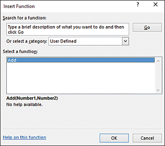
FIGURE 14-1 You can find your UDFs under the User Defined category of the Insert Function dialog box.
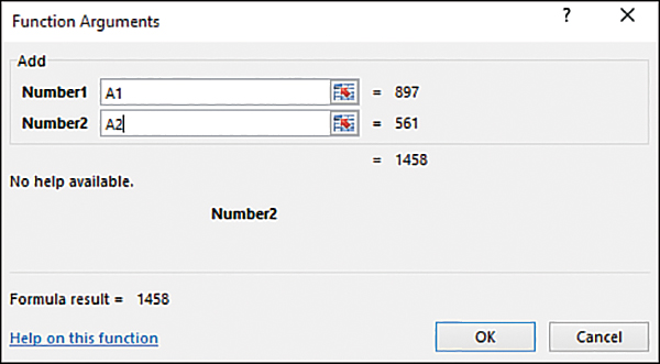
FIGURE 14-2 You can use the Function Arguments dialog box to enter your arguments.
![]() Note
Note
You can easily share custom functions because users are not required to know how the function works. See the next section, “Sharing UDFs,” for more information.
Most of the functions used on sheets can also be used in VBA and vice versa. However, in VBA you call the UDF (ADD) from a procedure (Addition), like this:
Sub Addition ()
Dim Total as Integer
Total = Add (1,10) 'we use a user-defined function Add
MsgBox "The answer is: " & Total
End Sub
Sharing UDFs
Where you store a UDF affects how you can share it:
Personal.xlsb—Store a UDF in
Personal.xlsbif it is just for your use and won’t be used in a workbook opened on another computer.Workbook—Store a UDF in the workbook in which it is being used if it needs to be distributed to many people.
Add-in—Distribute a UDF via an add-in if the workbook is to be shared among a select group of people. See Chapter 26, “Creating Excel add-ins” for information on how to create an add-in.
Template—Store a UDF in a template if it needs to be used to create several workbooks and the workbooks are distributed to many people.
Useful custom Excel functions
The sections that follow include a sampling of functions that can be useful in the everyday Excel world.
![]() Note
Note
This chapter shows functions donated by several Excel programmers. These are functions that they have found useful and that they hope will also be of help to you.
Different programmers have different programming styles. We did not rewrite the submissions. As you review the lines of code, you might notice different ways of doing the same task, such as referring to ranges.
Checking whether a workbook is open
There might be times when you need to check whether a workbook is open. The following function returns True if a workbook is open and False if it is not:
BookOpen(Bk)
The argument is Bk, which is the name of the workbook being checked:
Function BookOpen(Bk As String) As Boolean
Dim T As Excel.Workbook
Err.Clear 'clears any errors
On Error Resume Next 'if the code runs into an error, it skips it and
'continues
Set T = Application.Workbooks(Bk)
BookOpen = Not T Is Nothing
'If the workbook is open, then T will hold the workbook object and
'therefore will NOT be Nothing
Err.Clear
On Error GoTo 0
End Function
Here is an example of using the function:
Sub OpenAWorkbook()
Dim IsOpen As Boolean
Dim BookName As String
BookName = "ProjectFilesChapter14.xlsm"
IsOpen = BookOpen(BookName) 'calling our function - don't forget the 'parameter
If IsOpen Then
    MsgBox BookName & " is already open!"
Else
    Workbooks.Open BookName
End If
End Sub
Checking whether a sheet in an open workbook exists
This function requires that the workbook(s) it checks be open. It returns True if the sheet is found and False if it is not:
SheetExists(SName, WBName)
These are the arguments:
SName—The name of the sheet being searched.WBName—(Optional) The name of the workbook that contains the sheet.
Here is the function. If the workbook argument is not provided, it uses the active workbook:
Function SheetExists(SName As String, Optional WB As Workbook) As Boolean
 Dim WS As Worksheet
 ' Use active workbook by default
 If WB Is Nothing Then
    Set WB = ActiveWorkbook
 End If
 On Error Resume Next
 SheetExists = CBool(Not WB.Sheets(SName) Is Nothing)
 On Error GoTo 0
End Function![]() Note
Note
CBool is a function that converts the expression between the parentheses to a Boolean value.
Here is an example of using this function:
Sub CheckForSheet()
Dim ShtExists As Boolean
ShtExists = SheetExists("Sheet9")
'notice that only one parameter was passed; the workbook name is optional
If ShtExists Then
    MsgBox "The worksheet exists!"
Else
    MsgBox "The worksheet does NOT exist!"
End If
End Sub
Counting the number of workbooks in a directory
This function searches the current directory, and its subfolders if you want, counting all Excel macro workbook files (.xlsm), including hidden files, or just the ones starting with a string of letters:
NumFilesInCurDir (LikeText, Subfolders)
These are the arguments:
LikeText—(Optional) A string value to search for; must include an asterisk (*), such as Mr*.Subfolders—(Optional)Trueto search subfolders,False(default) not to.
![]() Note
Note
FileSystemObject requires the Microsoft Scripting Runtime reference library. To enable this setting, go to Tools, References and check Microsoft Scripting Runtime.
This function is a recursive function, which means it calls itself until a specific condition is met—in this case, until all subfolders are processed. Here is the function:
Function NumFilesInCurDir(Optional strInclude As String = "", _
 Optional blnSubDirs As Boolean = False)
Dim fso As FileSystemObject
Dim fld As Folder
Dim fil As File
Dim subfld As Folder
Dim intFileCount As Integer
Dim strExtension As String
 strExtension = "XLSM"
 Set fso = New FileSystemObject
 Set fld = fso.GetFolder(ThisWorkbook.Path)
 For Each fil In fld.Files
    If UCase(fil.Name) Like "*" & UCase(strInclude) & "*." & _
     UCase(strExtension) Then
      intFileCount = intFileCount + 1
    End If
 Next fil
 If blnSubDirs Then
    For Each subfld In fld.Subfolders
      intFileCount = intFileCount + NumFilesInCurDir(strInclude, True)
    Next subfld
 End If
 NumFilesInCurDir = intFileCount
 Set fso = Nothing
End Function
Here is an example of using this function:
Sub CountMyWkbks()
Dim MyFiles As Integer
MyFiles = NumFilesInCurDir("MrE*", True)
MsgBox MyFiles & " file(s) found"
End Sub
Retrieving the user ID
Ever need to keep a record of who saves changes to a workbook? With the USERID function, you can retrieve the name of the user who is logged in to a computer. Combine it with the function discussed in the “Retrieving permanent date and time” section, later in this chapter, and you have a nice log file. You can also use the USERID function to set up user rights to a workbook:
WinUserName ()No arguments are used with this function.
![]() Note
Note
The USERID function is an advanced function that uses the application programming interface (API), which is reviewed in Chapter 23, “The Windows Application Programming Interface (API).” The code is specific to 32-bit Excel. If you are running 64-bit Excel, refer to Chapter 23 for changes to make it work.
This first section (Private declarations) must be at the top of the module:
Private Declare Function WNetGetUser Lib "mpr.dll" Alias "WNetGetUserA" _
 (ByVal lpName As String, ByVal lpUserName As String, _
 lpnLength As Long) As Long
Private Const NO_ERROR = 0
Private Const ERROR_NOT_CONNECTED = 2250&
Private Const ERROR_MORE_DATA = 234
Private Const ERROR_NO_NETWORK = 1222&
Private Const ERROR_EXTENDED_ERROR = 1208&
Private Const ERROR_NO_NET_OR_BAD_PATH = 1203&
You can place the following section of code anywhere in the module, as long as it is below the preceding section:
Function WinUsername() As String
 'variables
 Dim strBuf As String, lngUser As Long, strUn As String
 'clear buffer for user name from api func
 strBuf = Space$(255)
 'use api func WNetGetUser to assign user value to lngUser
 'will have lots of blank space
 lngUser = WNetGetUser("", strBuf, 255)
 'if no error from function call
 If lngUser = NO_ERROR Then
    'clear out blank space in strBuf and assign val to function
    strUn = Left(strBuf, InStr(strBuf, vbNullChar) - 1)
    WinUsername = strUn
 Else
  'error, give up
    WinUsername = "Error :" & lngUser
 End If
End Function
Here’s an example of using this function:
Sub CheckUserRights()
Dim UserName As String
UserName = WinUsername
Select Case UserName
  Case "Administrator"
    MsgBox "Full Rights"
  Case "Guest"
    MsgBox "You cannot make changes"
  Case Else
    MsgBox "Limited Rights"
End Select
End Sub
Retrieving date and time of last save
This function retrieves the saved date and time of any workbook, including the current one:
LastSaved(FullPath)
![]() Note
Note
The cell must be formatted for date and time to display the date/time correctly.
The argument is FullPath, a string showing the full path and file name of the file in question:
Function LastSaved(FullPath As String) As Date
LastSaved = FileDateTime(FullPath)
End Function
Retrieving permanent date and time
Because of the volatility of the NOW function, it isn’t very useful for stamping a worksheet with the creation or editing date. Every time the workbook is opened or recalculated, the result of the NOW function is updated. The following UDF uses the NOW function. However, because you need to reenter the cell to update the function, it is much less volatile (see Figure 14-3).
No arguments are used with this function:
DateTime()
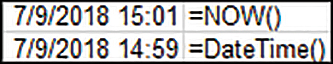
FIGURE 14-3 Even after forcing a recalculation, the DateTime() cell shows the time when it was originally placed in the cell, whereas NOW() shows the current system time.
![]() Note
Note
The cell must be formatted properly to display the date/time.
Here is the function:
Function DateTime()
 DateTime = Now
End Function
Validating an email address
If you manage an email subscription list, you might receive invalid email addresses, such as addresses with a space before the “at” symbol (@). The IsEmailValid function can check addresses and confirm that they are proper email addresses (see Figure 14-4):
IsEmailValid (strEmail)
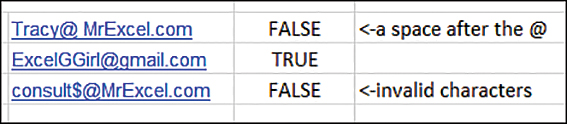
FIGURE 14-4 Validating email addresses.
![]() Note
Note
This function cannot verify that an email address is an existing one. It only checks the syntax to verify that the address might be legitimate.
The function’s only argument is strEmail, an email address:
Function IsEmailValid(strEmail As String) As Boolean
Dim strArray As Variant
Dim strItem As Variant
Dim i As Long
Dim c As String
Dim blnIsItValid As Boolean
blnIsItValid = True
'count the @ in the string
i = Len(strEmail) - Len(Application.Substitute(strEmail, "@", ""))
'if there is more than one @, invalid email
If i <> 1 Then IsEmailValid = False: Exit Function
ReDim strArray(1 To 2)
'the following two lines place the text to the left and right
'of the @ in their own variables
strArray(1) = Left(strEmail, InStr(1, strEmail, "@", 1) - 1)
strArray(2) = Application.Substitute(Right(strEmail, Len(strEmail) - _
 Len(strArray(1))), "@", "")

For Each strItem In strArray
   'verify there is something in the variable.
   'If there isn't, then part of the email is missing
   If Len(strItem) <= 0 Then
     blnIsItValid = False
     IsEmailValid = blnIsItValid
     Exit Function
   End If
   'verify only valid characters in the email
   For i = 1 To Len(strItem)
      'lowercases all letters for easier checking
      c = LCase(Mid(strItem, i, 1))
         If InStr("abcdefghijklmnopqrstuvwxyz_-.", c) <= 0 _
             And Not IsNumeric(c) Then
             blnIsItValid = False
             IsEmailValid = blnIsItValid
             Exit Function
         End If
   Next i
  'verify that the first character of the left and right aren't periods
   If Left(strItem, 1) = "." Or Right(strItem, 1) = "." Then
      blnIsItValid = False
      IsEmailValid = blnIsItValid
      Exit Function
   End If
Next strItem
'verify there is a period in the right half of the address
If InStr(strArray(2), ".") <= 0 Then
    blnIsItValid = False
    IsEmailValid = blnIsItValid
    Exit Function
End If
i = Len(strArray(2)) - InStrRev(strArray(2), ".") 'locate the period
'verify that the number of letters corresponds to a valid domain
'extension
If i <> 2 And i <> 3 And i <> 4 Then
    blnIsItValid = False
    IsEmailValid = blnIsItValid
    Exit Function
End If
'verify that there aren't two periods together in the email
If InStr(strEmail, "..") > 0 Then
    blnIsItValid = False
    IsEmailValid = blnIsItValid
    Exit Function
End If
IsEmailValid = blnIsItValid
End Function
Summing cells based on interior color
Let’s say you have created a list of how much each of your clients owes. From this list, you want to sum just the cells to which you have applied a cell fill to indicate clients who are 30 days past due. This function sums cells based on their fill color:
SumColor(CellColor, SumRange)
![]() Note
Note
Cells colored by conditional formatting will not work with this function; the cells must have an interior color.
These are the arguments:
CellColor—The address of a cell with the target color.SumRange—The range of cells to be searched.
Here is the function’s code:
Function SumByColor(CellColor As Range, SumRange As Range)
Dim myCell As Range
Dim iCol As Integer
Dim myTotal
iCol = CellColor.Interior.ColorIndex 'get the target color
For Each myCell In SumRange 'look at each cell in the designated range
  'if the cell color matches the target color
  If myCell.Interior.ColorIndex = iCol Then
     'add the value in the cell to the total
     myTotal = WorksheetFunction.Sum(myCell, myTotal)
  End If
Next myCell
SumByColor = myTotal
End Function
Figure 14-5 shows a sample worksheet using this function.
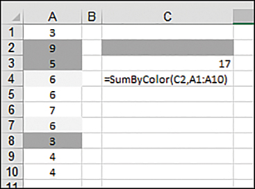
FIGURE 14-5 The function sums cells based on interior color.
Counting unique values
How many times have you had a long list of values and needed to know how many were unique values? This function goes through a range and provides that information, as shown in Figure 14-6:
NumUniqueValues(Rng)
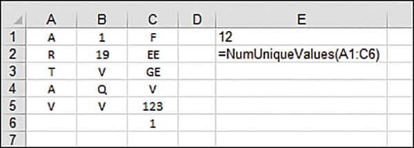
FIGURE 14-6 The function counts the number of unique values in a range.
The argument is Rng, the range to search unique values.
Here is the function’s code:
Function NumUniqueValues(Rng As Range) As Long
Dim myCell As Range
Dim UniqueVals As New Collection
Application.Volatile 'forces the function to recalculate when the range changes
On Error Resume Next
'the following places each value from the range into a collection
'because a collection, with a key parameter, can contain only unique
'values,there will be no duplicates. The error statements force the
'program to continue when the error messages appear for duplicate
'items in the collection
For Each myCell In Rng
   UniqueVals.Add myCell.Value, CStr(myCell.Value)
Next myCell
On Error GoTo 0
'returns the number of items in the collection
NumUniqueValues = UniqueVals.Count
End Function
Finding the first nonzero-length cell in a range
Suppose you have imported a large list of data with many empty cells. Here is a function that evaluates a range of cells and returns the value of the first nonzero-length cell:
FirstNonZeroLength(Rng)
The argument is Rng, the range to search.
Here’s the function:
Function FirstNonZeroLength(Rng As Range)
Dim myCell As Range
FirstNonZeroLength = 0#
For Each myCell In Rng
   If Not IsNull(myCell) And myCell <> "" Then
      FirstNonZeroLength = myCell.Value
      Exit Function
   End If
Next myCell
FirstNonZeroLength = myCell.Value
End Function
Figure 14-7 shows the function on a sample worksheet.
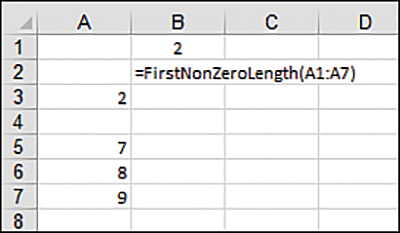
FIGURE 14-7 You can use a user-defined function to find the value of the first nonzero-length cell in a range.
Substituting multiple characters
Excel has a substitute function, but it is a value-for-value substitution. What if you have several characters you need to substitute? Figure 14-8 shows several examples of how this function works:
MSubstitute(trStr, frStr, toStr)
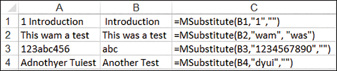
FIGURE 14-8 You can substitute multiple characters in a cell.
These are the arguments:
trStr—The string to be searched.FrStr—The text being searched for.toStr—The replacement text.
Here’s the function’s code:
Function MSubstitute(ByVal trStr As Variant, frStr As String, _
 toStr As String) As Variant
Dim iCol As Integer
Dim j As Integer
Dim Ar As Variant
Dim vfr() As String
Dim vto() As String
ReDim vfr(1 To Len(frStr))
ReDim vto(1 To Len(frStr))
'place the strings into an array
For j = 1 To Len(frStr)
    vfr(j) = Mid(frStr, j, 1)
    If Mid(toStr, j, 1) <> "" Then
      vto(j) = Mid(toStr, j, 1)
    Else
      vto(j) = ""
    End If
Next j
'compare each character and substitute if needed
If IsArray(trStr) Then
   Ar = trStr
   For iRow = LBound(Ar, 1) To UBound(Ar, 1)
      For iCol = LBound(Ar, 2) To UBound(Ar, 2)
          For j = 1 To Len(frStr)
            Ar(iRow, iCol) = Application.Substitute(Ar(iRow, iCol), _
             vfr(j), vto(j))
           Next j
      Next iCol
   Next iRow
Else
    Ar = trStr
    For j = 1 To Len(frStr)
       Ar = Application.Substitute(Ar, vfr(j), vto(j))
    Next j
End If
MSUBSTITUTE = Ar
End Function![]() Note
Note
The toStr argument is assumed to be the same length as frStr. If it isn’t, the remaining characters are considered null (""). The function is case sensitive. To replace all instances of a, use a and A. You cannot replace one character with two characters. For example, this:
=MSUBSTITUTE("This is a test","i","$@")results in this:
"Th$s $s a test"
Retrieving numbers from mixed text
This function extracts and returns numbers from text that is a mixture of numbers and letters:
RetrieveNumbers (myString)
The argument is myString, the text containing the numbers to be extracted.
Here’s the function’s code:
Function RetrieveNumbers(myString As String)
Dim i As Integer, j As Integer
Dim OnlyNums As String
'starting at the END of the string and moving backwards (Step -1)
For i = Len(myString) To 1 Step -1
    'IsNumeric is a VBA function that returns True if a variable is a number
    'When a number is found, it is added to the OnlyNums string
    If IsNumeric(Mid(myString, i, 1)) Then
        j = j + 1
        OnlyNums = Mid(myString, i, 1) & OnlyNums
    End If
    If j = 1 Then OnlyNums = CInt(Mid(OnlyNums, 1, 1))
Next i
RetrieveNumbers = CLng(OnlyNums)
End Function
Converting week number into date
Have you ever received a spreadsheet report in which all the headers showed the week number? This can be confusing because you probably wouldn’t know what Week 15 actually is. You would have to get out your calendar and count the weeks. This problem is exacerbated if you need to count weeks in a previous year. In this case, you need a nice little function that converts Week ## Year into the date of a particular day in a given week, as shown in Figure 14-9.
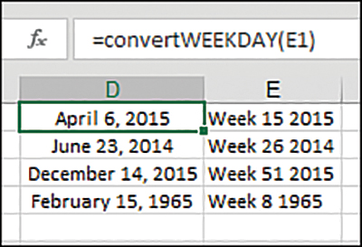
FIGURE 14-9 You can convert a week number into a date that’s more easily referenced.
![]() Note
Note
The result must be formatted as a date.
The argument is Str, the week to be converted, in Week ## YYYY format.
Here’s the function’s code:
Function ConvertWeekDay(Str As String) As Date
Dim Week As Long
Dim FirstMon As Date
Dim TStr As String
FirstMon = DateSerial(Right(Str, 4), 1, 1)
FirstMon = FirstMon - FirstMon Mod 7 + 2
TStr = Right(Str, Len(Str) - 5)
Week = Left(TStr, InStr(1, TStr, " ", 1)) + 0
ConvertWeekDay = FirstMon + (Week - 1) * 7
End Function
Sorting and concatenating
The following function enables you to take a column of data, sort it by numbers and then by letters, and concatenate it using a comma (,) as the delimiter (see Figure 14-10). Note that since the numbers are treated as strings, they are sorted lexicographically (all numbers that start with 1, then numbers that start with 2, etc.). For example, if sorting 1,2,10, you would actually get 1,10,2 because 10 starts with a 1, which comes before 2:
SortConcat(Rng)
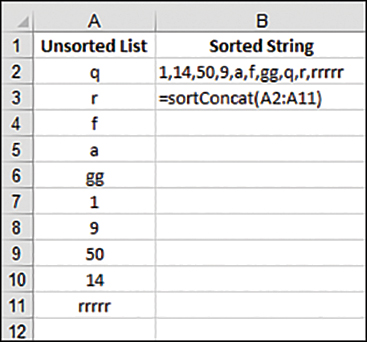
FIGURE 14-10 This function sorts and concatenates a range of variables.
The argument is Rng, the range of data to be sorted and concatenated. SortConcat calls another procedure, BubbleSort, that must be included.
Here’s the main function:
Function SortConcat(Rng As Range) As Variant
Dim MySum As String, arr1() As String
Dim j As Integer, i As Integer
Dim cl As Range
Dim concat As Variant
On Error GoTo FuncFail:
'initialize output
SortConcat = 0#
'avoid user issues
If Rng.Count = 0 Then Exit Function
'get range into variant variable holding array
ReDim arr1(1 To Rng.Count)
'fill array
i = 1
For Each cl In Rng
    arr1(i) = cl.Value
    i = i + 1
Next
'sort array elements
Call BubbleSort(arr1)
'create string from array elements
For j = UBound(arr1) To 1 Step -1
    If Not IsEmpty(arr1(j)) Then
          MySum = arr1(j) & ", " & MySum
    End If
Next j
'assign value to function
SortConcat = Left(MySum, Len(MySum) - 1)
'exit point
concat_exit:
Exit Function
'display error in cell
FuncFail:
SortConcat = Err.Number & " - " & Err.Description
Resume concat_exit
End Function
The following function is the ever-popular BubbleSort. Many developers use this program to do a simple sort of data:
Sub BubbleSort(List() As String)
' Sorts the List array in ascending order
Dim First As Integer, Last As Integer
Dim i As Integer, j As Integer
Dim Temp
First = LBound(List)
Last = UBound(List)
For i = First To Last - 1
  For j = i + 1 To Last
     If List(i) > List(j) Then
       Temp = List(j)
       List(j) = List(i)
       List(i) = Temp
     End If
  Next j
Next i
End Sub
Sorting numeric and alpha characters
This function takes a mixed range of numeric and alpha characters and sorts them—first numerically and then alphabetically:
sorter(Rng)
The result is placed in an array that can be displayed on a worksheet, as shown in Figure 14-11. Excel will automatically resize the results range as needed.
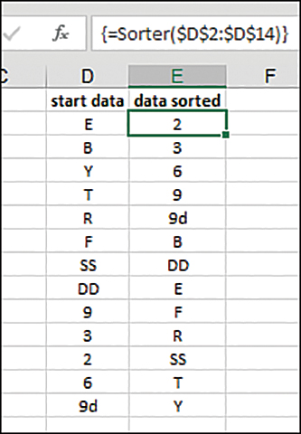
FIGURE 14-11 This function sorts a mixed alphanumeric list.
The argument is Rng, the range to be sorted.
The function uses the following two procedures to sort the data in the range:
Public Sub QuickSort(ByRef vntArr As Variant, _
 Optional ByVal lngLeft As Long = -2, _
 Optional ByVal lngRight As Long = -2)
Dim i, j, lngMid As Long
Dim vntTestVal As Variant
If lngLeft = -2 Then lngLeft = LBound(vntArr)
If lngRight = -2 Then lngRight = UBound(vntArr)
If lngLeft < lngRight Then
  lngMid = (lngLeft + lngRight)  2
  vntTestVal = vntArr(lngMid)
  i = lngLeft
  j = lngRight
  Do
     Do While vntArr(i) < vntTestVal
       i = i + 1
     Loop
     Do While vntArr(j) > vntTestVal
       j = j - 1
     Loop
     If i <= j Then
       Call SwapElements(vntArr, i, j)
       i = i + 1
       j = j - 1
     End If
  Loop Until i > j
  If j <= lngMid Then
     Call QuickSort(vntArr, lngLeft, j)
     Call QuickSort(vntArr, i, lngRight)
  Else
     Call QuickSort(vntArr, i, lngRight)
     Call QuickSort(vntArr, lngLeft, j)
  End If
End If
End Sub

Private Sub SwapElements(ByRef vntItems As Variant, _
    ByVal lngItem1 As Long, _
    ByVal lngItem2 As Long)
Dim vntTemp As Variant
vntTemp = vntItems(lngItem2)
vntItems(lngItem2) = vntItems(lngItem1)
vntItems(lngItem1) = vntTemp
End Sub
Here’s an example of using this function:
Function sorter(Rng As Range) As Variant
'returns an array
Dim arr1() As Variant
If Rng.Columns.Count > 1 Then Exit Function
arr1 = Application.Transpose(Rng)
QuickSort arr1
sorter = Application.Transpose(arr1)
End Function
Searching for a string within text
Ever needed to find out which cells contain a specific string of text? This function can search strings in a range, looking for specified text:
ContainsText(Rng,Text)
It returns a result that identifies which cells contain the text, as shown in Figure 14-12.
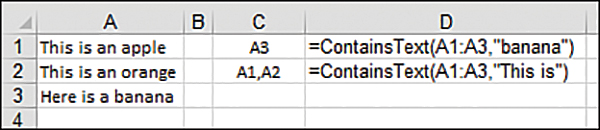
FIGURE 14-12 The ContainsText function returns a result that identifies which cells contain a specified string.
These are the arguments:
Rng—The range in which to search.Text—The text for which to search.
Here’s the function’s code:
Function ContainsText(Rng As Range, Text As String) As String
Dim T As String
Dim myCell As Range
For Each myCell In Rng 'look in each cell
  If InStr(myCell.Text, Text) > 0 Then 'look in the string for the text
      If Len(T) = 0 Then
         'if the text is found, add the address to my result
         T = myCell.Address(False, False)
      Else
         T = T & "," & myCell.Address(False, False)
      End If
  End If
Next myCell
ContainsText = T
End Function
Returning the addresses of duplicate maximum values
MAX finds and returns the maximum value in a range, but it doesn’t tell you whether there is more than one maximum value. This function returns the addresses of the maximum values in a range, as shown in Figure 14-13:
ReturnMaxs(Rng)
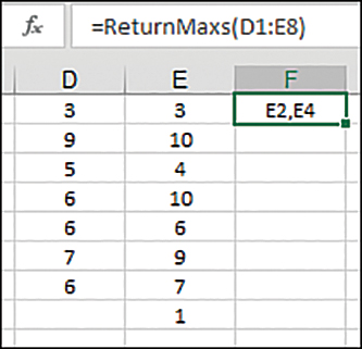
FIGURE 14-13 This function returns the addresses of all maximum values in a range.
The argument is Rng, the range to search for the maximum values.
Here’s the function’s code:
Function ReturnMaxs(Rng As Range) As String
Dim Mx As Double
Dim myCell As Range
'if there is only one cell in the range, then exit
If Rng.Count = 1 Then ReturnMaxs = Rng.Address(False, False): _
 Exit Function
Mx = Application.Max(Rng) 'uses Excel's MAX to find the max in the range
'Because you now know what the max value is,
'search the range to find matches and return the address
For Each myCell In Rng
  If myCell = Mx Then
      If Len(ReturnMaxs) = 0 Then
        ReturnMaxs = myCell.Address(False, False)
      Else
        ReturnMaxs = ReturnMaxs & ", " & myCell.Address(False, False)
      End If
  End If
Next myCell
End Function
Returning a hyperlink address
Let’s say that you’ve received a spreadsheet containing a list of hyperlinked information. You want to see the actual links, not the descriptive text. You could just right-click a hyperlink and select Edit Hyperlink, but you want something more permanent. This function extracts the hyperlink address, as shown in Figure 14-14:
GetAddress(HyperlinkCell)
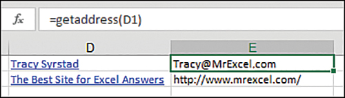
FIGURE 14-14 You can extract the hyperlink address from behind a hyperlink.
The argument is HyperlinkCell, the hyperlinked cell from which you want the address extracted.
Here’s the function’s code:
Function GetAddress(HyperlinkCell As Range)
 GetAddress = Replace(HyperlinkCell.Hyperlinks(1).Address, "mailto:", "")
End Function
Returning the column letter of a cell address
You can use CELL("Col") to return a column number, but what if you need the column letter? This function extracts the column letter from a cell address, as shown in Figure 14-15:
ColName(Rng)
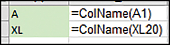
FIGURE 14-15 You can get the column letter of a cell address.
The argument is Rng, the cell for which you want the column letter.
Here’s the function’s code:
Function ColName(Rng As Range) As String
ColName = Left(Rng.Range("A1").Address(True, False), _
 InStr(1, Rng.Range("A1").Address(True, False), "$", 1) - 1)
End Function
Using Select…Case on a worksheet
At some point, you have probably nested an If...Then...Else on a worksheet to return a value. The Select...Case statement available in VBA makes this a lot easier, but you can’t use Select...Case statements in a worksheet formula. Instead, you can create a UDF (see Figure 14-16).
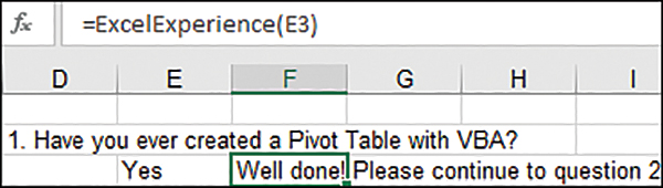
FIGURE 14-16 The ExcelExperience function uses the Select...Case structure rather than nested If...Then statements.
This example takes the user input and returns a response, as shown in Figure 14-16. Although you could use the following formula instead, consider how long it could get if you had more options. Or what if you needed to compare the results of a calculation? You would have to do the calculation for each logical comparison:
=IF(E3="yes","Well done! Please continue to question 2",IF(E3="no","Check out
Chapter 12 for some help.  Please skip to question 10", "Please clarify your
response in the box below"))
Because Select...Case is case sensitive, I’ve developed the habit of always using uppercase (UCase) when comparing strings. Here is the code:
Function ExcelExperience(ByVal UserResponse As String) As String
Select Case UCase(UserResponse)
    Case Is = "YES"
        ExcelExperience = "Well done! Please continue to question 2"
    Case Is = "NO"
        ExcelExperience = "Check out Chapter 12 for some help. " & _
            "Please skip to question 10"
    Case Is = "MAYBE"
        ExcelExperience = "Please clarify your response " & _
            "in the box below"
    Case Else
        ExcelExperience = "Invalid response"
End Select
End Function
Creating LAMBDA functions
While UDFs are very useful, you might need to create and distribute custom formulas in a macro-free workbook. You could create the formula and then instruct users on how to copy/paste it where needed, modifying the correct cell references. Or, you can create a LAMBDA function and provide the users with the name of the function and what arguments are required.
LAMBDA allows you to design a custom function in the Name Manager using Excel’s native functions and other custom LAMBDA functions. You then call that function similar to how you would call a UDF—but there is no VBA needed.
![]() Note
Note
Unlike VBA, multiple lines and spacing don’t matter in formulas. Therefore, in the following code blocks, lines wrap naturally and underscores are not used to join multiple lines together.
Building a simple LAMBDA function
To learn the basics of LAMBDA functions, you’ll build a custom function that returns the parent worksheet name of a referenced cell. The structure of the function is:
=LAMBDA(parameters, calculation)
You can have up to 253 comma delimited parameters—just make sure the calculation is the last argument.
In Excel, open the Name Manager in the Formulas tab and click the New button. In the Name field, enter the name of the function, SHEETNAME. In the Refers to field, enter the following:
=LAMBDA(reference, LET(name, CELL("filename",reference),RIGHT(name, LEN(name) -
FIND("]", name))))
Figure 14-17 shows the fields filled in. Click OK to save your changes and return to Excel.
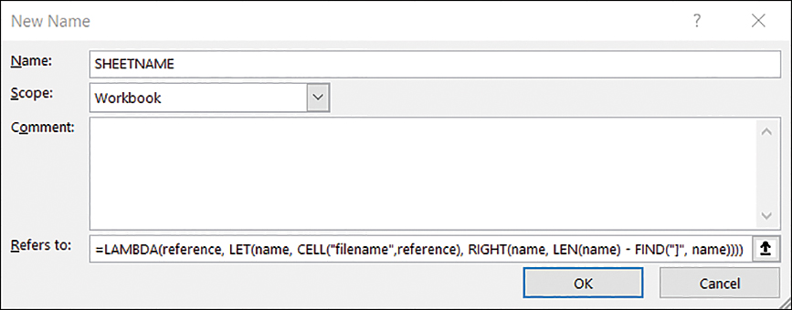
FIGURE 14-17 LAMBDA functions are defined in the Name Manager.
Let’s break down the previous formula:
LAMBDAis the Excel function that makes this all work.referenceis the parameter used by the calculation; in this case, it will be a cell reference. You could simply usexif you wanted to, but helpful terms make it easier when you come back later and review the function.LET(name, CELL("filename",reference),RIGHT(name, LEN(name) - FIND("]", name)))is the actual calculation being done.
![]() Note
Note
LET is a new Excel function allowing you to assign values to names that are then used in a calculation, all within the LET function itself. In the case of the previous formula, name is the variable name, CELL("filename",reference) is the value of that variable, and RIGHT(name, LEN(name) - FIND("]", name)) is the calculation using the variable.
Here’s how to use the function on a worksheet:
![]() Note
Note
Currently, there is little built-in help in using LAMBDA functions, so you will need to know the function name and its argument(s).
Select the cell on the sheet where you want the sheet name to be.
Type = and then the function name, just as you would one of Excel’s built-in functions, like this:
=SHEETNAME.Type the opening parenthesis, select a cell on the sheet which you want to return the sheet name from, then type the closing parenthesis. Your formula should look something like this:
=SHEETNAME(Sheet2!C18).Press the Enter key.
The name of the sheet will appear in the cell. You can also use this function to return the name of the sheet on which a range name appears. For example,
=SHEETNAME(TaxRate)would return the name of the sheet where theTaxRaterange name can be found.
Sharing LAMBDA functions
There are two requirements for sharing LAMBDA functions. First, the end-user must have a version of Excel that includes LAMBDA. Second, the workbook using the function must include it—you cannot reference a function stored in another workbook, such as the Personal.xlsb. Someone looking at a LAMBDA function you created with an older version of Excel will see something like this:
=_xlfn.LAMBDA(_xlpm.reference, LET(name, CELL("filename",_xlpm.reference),
RIGHT(name, LEN(name) - FIND("]", name))))
Useful LAMBDA functions
The previous SHEETNAME function and the following two functions were written by Suat Ozgur. Suat is a Full-stack Web Developer and a certified Database Administrator. These functions and many others can be found in the Excel LAMBDA Functions forum at the MrExcel message board (www.mrexcel.com/board/forums/excel-lambda-functions.40/).
SLUGIFY.PLUS
SLUGIFY.PLUS takes text and replaces non-alphanumeric characters with dashes so the text can be used as the URL slug in a web address, as shown in Figure 14-18. It uses recursion and branching to remove any multiple adjacent dashes that may appear. Recursion is when a program (or formula, in this case) calls itself. In the following code, you’ll notice there are calls to SLUGIFY.PLUS within the formula itself.
Branching is when a statement, such as an IF statement, instructs the code on what to do based on the value of an expression. In this function, the value of the subroutine argument is used to initialize the start of the branch (IF(subroutine=1)). A recursion call sets this argument’s value to 0, instructing the code to follow another branch of logic:
SLUGIFY.PLUS(reference, ndx, subroutine)
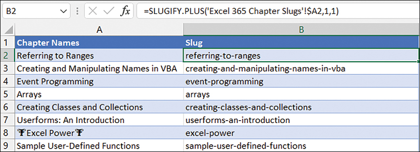
FIGURE 14-18 SLUGIFY.PLUS renders a useable URL slug from text.
These are the arguments:
reference—The cell reference (or string value) that contains the string to be converted to a URL slug.ndx—The starting character index. Enter 1 to convert the entire string.subroutine—The subroutine index of the process that we want to call. The initial value must be 1.
Here is the function’s formula:
=LAMBDA(reference,ndx,subroutine,
  IF(subroutine=1,
    IF(ndx > LEN(reference),
      SLUGIFY.PLUS(reference, 0,2),
      SLUGIFY.PLUS(
        LET(
          character, LOWER(MID(reference, ndx, 1)),
          charcode, CODE(character),
          LEFT(reference, ndx - 1) & IF(OR(AND(charcode > 96, charcode < 123),
AND(charcode > 47, charcode < 58)), character, "-") & RIGHT(reference,
LEN(reference) - ndx)
        ),
        ndx + 1,
        1
      )
    ),
    IF(LEN(reference)-LEN(SUBSTITUTE(reference, "--", "")) = 0,
      LET(
        clearleft, IF(LEFT(reference, 1)="-", RIGHT(reference, LEN(reference)-1),
reference),
        clearright,  IF(RIGHT(clearleft, 1)="-", LEFT(clearleft,
LEN(clearleft)-1), clearleft),
        clearright
      ),
      SLUGIFY.PLUS(
        SUBSTITUTE(reference, "--", "-"), 0, 2
      )
    )
  )
)
TOC2HTML
TOC2HTML creates the HTML code for a table of contents, as shown in Figure 14-19. This function uses recursion and looping to accomplish this task. To create the loop, the argument loopCounter is used to initialize the counter within the code, i, to 0. The LET function is then used to increment the i (LET(i, i+1, …) and the variable is then used as the loopCounter value in the recursive call:
TOC2HTML(reference, chapterKeyword, loopCounter)
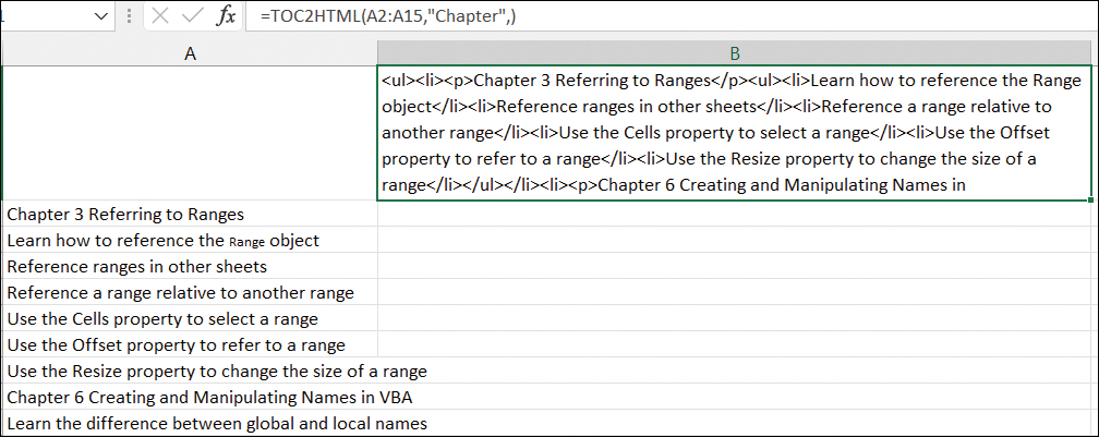
FIGURE 14-19 TOC2HTML takes a range and generates an HTML list.
These are the arguments:
reference—The range consisting of multiple rows and a single column containing the table of contents list.chapterKeyword—The repeating keyword defining the main chapters to create the nested sections.loopCounter—The counter to create the loop. The initial value should be 0 or blank.
Here is the function’s formula:
=LAMBDA(rng,chapterKeyword,i,
    LET(rows, ROWS(rng),
        IF(i = rows,
            "",
            LET(i, i+1,
                cll, INDEX(rng,i),
                isFirstLevel, IFERROR(FIND(chapterKeyword, cll),0),
                IF(isFirstLevel,
                     IF(i=1,
                    "<ul>","</ul></li>") & "<li><p>" & cll & "</p><ul>",
                    "<li>" & cll & "</li>"
                )
                & TOC2HTML(rng, chapterKeyword, i)
                & IF(i = rows - 1,
                     "</ul></li></ul>",
                     ""
                    )
            )
        )
    )
)
Next steps
User-defined and LAMBDA functions allow you to take potentially complicated formulas and make them easier for users to apply. Now that you’ve learned how to work the data, it’s time to visualize it. In Chapter 15, “Creating charts,” you’ll find out how spreadsheet charting has become highly customizable and capable of handling large amounts of data.