
14
Generalized Linear Models
Not every response variable will be continuous, so a linear regression will not be the correct model in every circumstance. Some outcomes may contain binary data (e.g., sick and not sick), or even count data (e.g., how many heads will I get when I flip a coin). A general class of models called generalized linear models (GLM) can account for these types of data, yet still use a linear combination of predictors.
About This Chapter
This chapter has been improved from its first edition version in a few ways. First, the data set example was changed to use the titanic data set from the seaborn library. The original code from the New York American Community Survey (ACS) was replaced with a new data set to make the model outputs more comparable across multiple libraries and programming languages (Appendix Z).
Next, the first edition of this book did not emphasize the different parameter options in functions from the scikit-learn library. This was originally a bit misleading as it gave off the impression that the models were doing exactly the same thing when they have different default behaviors. This chapter now gives more code and examples to emphasize the model differences between the modeling libraries. The original ACS modeling code can still be found in Appendix Y.
14.1 Logistic Regression (Binary Outcome Variable)
When you have a binary response variable (i.e., two possible outcomes), logistic regression is often used to model the data. We will be using the titanic data set that was exported from the seaborn library.
With our data loaded, let’s first subset the dataframe using only the columns we will be using for this model. We will also be dropping rows with missing values in them since models usually ignore observations that are not complete anyway, and we are not showing how to impute missing data in this chapter. Notice that we are dropping the missing values after we subsetted the columns we wanted, so we are not artificially dropping observations.
titanic_sub = (
    titanic[["survived", "sex", "age", "embarked"]].copy().dropna()
)

print(titanic_sub)
survived sex age embarked
0 0 male 22.0 S
1 1 female 38.0 C
2 1 female 26.0 S
3 1 female 35.0 S
4 0 male 35.0 S
.. ... ... ... ...
885 0 female 39.0 Q
886 0 male 27.0 S
887 1 female 19.0 S
889 1 male 26.0 C
890 0 male 32.0 Q[712 rows x 4 columns]In this data set, our outcome of interest is the survived column, on whether an individual survived (1) or died (0) during the sinking of the Titanic. The other columns, sex, age, and embarked are going to be the variable we use to see who survived.
# count of values in the survived column
print(titanic_sub["survived"].value_counts())
0 424
1 288
Name: survived, dtype: int64The embarked column describes where the individual boarded the ship from. There are three values for embarked: Southampton (S), Cherbourg (C), and Queenstown (Q).
# count of values in the embarked column
print(titanic_sub["embarked"].value_counts())
S 554
C 130
Q 28
Name: embarked, dtype: int64Interpreting results from a logistic regression model is not as straightforward as interpreting a linear regression model. In a logistic regression, as with all generalized linear models, there is a transformation (i.e., link function), that that affects how to interpret the results.
The link function for logistic regression is usually the logit link function.
Where p is the probability of the event, and
14.1.1 With statsmodels
To perform a logistic regression in statsmodels we can use the logit() function. The syntax for this function is the same as that used for linear regression in Chapter 13.
import statsmodels.formula.api as smf

# formula for the model
form = 'survived ~ sex + age + embarked'

# fitting the logistic regression model, note the .fit() at the end
py_logistic_smf = smf.logit(formula=form, data=titanic_sub).fit()

print(py_logistic_smf.summary())
Optimization terminated successfully.
Current function value: 0.509889
Iterations 6
Logit Regression Results
============================================================================
Dep. Variable: survived No. Observations: 712
Model: Logit Df Residuals: 707
Method: MLE Df Model: 4
Date: Thu, 01 Sep 2022 Pseudo R-squ.: 0.2444
Time: 01:55:49 Log-Likelihood: -363.04
converged: True LL-Null: -480.45
Covariance Type: nonrobust LLR p-value: 1.209e-49
==============================================================================
coef std err z P>|z| [0.025 0.975]
------------------------------------------------------------------------------
Intercept 2.2046 0.322 6.851 0.000 1.574 2.835
sex[T.male] -2.4760 0.191 -12.976 0.000 -2.850 -2.102
embarked[T.Q] -1.8156 0.535 -3.393 0.001 -2.864 -0.767
embarked[T.S] -1.0069 0.237 -4.251 0.000 -1.471 -0.543
age -0.0081 0.007 -1.233 0.217 -0.021 0.005
==============================================================================We can then get the coefficients of the model, and exponentiate it to calculate the odds of each variable.
import numpy as np

# get the coefficients into a dataframe
res_sm = pd.DataFrame(py_logistic_smf.params, columns=["coefs_sm"])

# calculate the odds
res_sm["odds_sm"] = np.exp(res_sm["coefs_sm"])

# round the decimals
print(res_sm.round(3))
coefs_sm odds_sm
Intercept 2.205 9.066
sex[T.male] -2.476 0.084
embarked[T.Q] -1.816 0.163
embarked[T.S] -1.007 0.365
age -0.008 0.992An example interpretation of these numbers would be that for every one unit increase in age, the odds of the survived decreases by 0.992 times. Since the value is close to 1, it seems that age wasn’t too much of a factor in survival. You can also confirm that statement by looking at the p-value for the variable in the summary table (under the P>|z| column).
A similar interpretation can be made with categorical variables. Recall that categorical variables are always interpreted in relation to the reference variable.
There are two potential values for sex in this data set, male and female, but only a coefficient for male is given. So that means the value is interpreted as “males compared to females”, where female is the reference variable. The odds for the male variable are interpreted as: males were 0.084 times more likely to survive compared to females (the odds for not surviving the tragedy were high for males).
14.1.2 With sklearn
When using sklearn, remember that dummy variables need to be created manually.
titanic_dummy = pd.get_dummies(
    titanic_sub[["survived", "sex", "age", "embarked"]],
    drop_first=True
)# note our outcome variable is the first column (index 0)
print(titanic_dummy) survived age sex_male embarked_Q embarked_S
0 0 22.0 1 0 1
1 1 38.0 0 0 0
2 1 26.0 0 0 1
3 1 35.0 0 0 1
4 0 35.0 1 0 1
.. ... ... ... ... ...
885 0 39.0 0 1 0
886 0 27.0 1 0 1
887 1 19.0 0 0 1
889 1 26.0 1 0 0
890 0 32.0 1 1 0[712 rows x 5 columns]We can then use the LogisticRegression() function from the linear_model module to create a logistic regression output to fit our model.
from sklearn import linear_model

# this is the only part that fits the model
py_logistic_sklearn1 = (
  linear_model.LogisticRegression().fit(
    X=titanic_dummy.iloc[:, 1:], # all the columns except first
    y=titanic_dummy.iloc[:, 0]   # just the first column
  )
)The code below will process the scikit-learn logistic regression fitted model into a single dataframe so we can better compare results.
# get the names of the dummy variable columns
dummy_names = titanic_dummy.columns.to_list()
# get the intercept and coefficients into a dataframe
sk1_res1 = pd.DataFrame(
    py_logistic_sklearn1.intercept_,
    index=["Intercept"],
    columns=["coef_sk1"],

)
sk1_res2 = pd.DataFrame(
    py_logistic_sklearn1.coef_.T,
    index=dummy_names[1:],
    columns=["coef_sk1"],

)

# put the results into a single dataframe to show the results
res_sklearn_pd_1 = pd.concat([sk1_res1, sk1_res2])

# calculate the odds
res_sklearn_pd_1["odds_sk1"] = np.exp(res_sklearn_pd_1["coef_sk1"])

print(res_sklearn_pd_1.round(3))
coef_sk1 odds_sk1
Intercept 2.024 7.571
age -0.008 0.992
sex_male -2.372 0.093
embarked_Q -1.369 0.254
embarked_S -0.887 0.412You will notice here that the coefficient values are different from the ones calculated from the statsmodels section we just did. The differences are more than a simple rounding error too!
14.1.3 Be Careful of scikit-learn Defaults
The main reason why the sklearn results differ from the statsmodels results stems from the domain differences where the two packages come from. Scikit-learn comes more from the machine learning world and is focused on prediction so the model defaults are set for numeric stability, and not for inference. However, statsmodels functions are implemented in a manner more traditional for statistics.
The LogisticRegression() function has a penalty parameter that defaults to 'l2', which adds an L2 penalty term (more about penalty terms in Chapter 17). If we want LogisticRegression() to behave in a manner more traditional for statistics, we need to set penalty="none".
# fit another logistic regression with no penalty
py_logistic_sklearn2 = linear_model.LogisticRegression(
     penalty="none" # this parameter is important!
).fit(
     X=titanic_dummy.iloc[:, 1:],   # all the columns except first
     y=titanic_dummy.iloc[:, 0]    # just the first column
)

# rest of the code is the same as before, except variable names
sk2_res1 = pd.DataFrame(
    py_logistic_sklearn2.intercept_,
    index=["Intercept"],
    columns=["coef_sk2"],
)
sk2_res2 = pd.DataFrame(
    py_logistic_sklearn2.coef_.T,
    index=dummy_names[1:],
    columns=["coef_sk2"],
)

res_sklearn_pd_2 = pd.concat([sk2_res1, sk2_res2])
res_sklearn_pd_2["odds_sk2"] = np.exp(res_sklearn_pd_2["coef_sk2"])First, let’s look at the original statsmodels results
sm_results = res_sm.round(3)

# sort values to make things easier to compare
sm_results = sm_results.sort_index()

print(sm_results)
coefs_sm odds_sm
Intercept 2.205 9.066
age -0.008 0.992
embarked[T.Q] -1.816 0.163
embarked[T.S] -1.007 0.365
sex[T.male] -2.476 0.084Now, let’s compare them with the two sklearn results
# concatenate the 2 model results
sk_results = pd.concat(
   [res_sklearn_pd_1.round(3), res_sklearn_pd_2.round(3)],
   axis="columns",
)

# sort cols and rows to make things easy to compare
sk_results = sk_results[sk_results.columns.sort_values()]
sk_results = sk_results.sort_index()

print(sk_results) coef_sk1 coef_sk2 odds_sk1 odds_sk2
Intercept 2.024 2.205 7.571 9.066
age -0.008 -0.008 0.992 0.992
embarked_Q -1.369 -1.816 0.254 0.163
embarked_S -0.887 -1.007 0.412 0.365
sex_male -2.372 -2.476 0.093 0.084The results here can also be compared to the same data and model from the R programming language in Appendix Z.2. You can see how subtle differences between the model parameters can cause differences in the interpretations.
14.2 Poisson Regression (Count Outcome Variable)
Poisson regression is performed when our response variable involves count data.
acs = pd.read_csv('data/acs_ny.csv')
print(acs.columns)
Index(['Acres', 'FamilyIncome', 'FamilyType', 'NumBedrooms',
'NumChildren', 'NumPeople', 'NumRooms', 'NumUnits',
'NumVehicles', 'NumWorkers', 'OwnRent', 'YearBuilt',
'HouseCosts', 'ElectricBill', 'FoodStamp', 'HeatingFuel',
'Insurance', 'Language'],
dtype='object')For example, in the acs data, the NumChildren variable is an example of count data.
14.2.1 With statsmodels
We can perform a Poisson regression using the poisson() function in statsmodels. We will use the NumBedrooms variable (Figure 14.1).
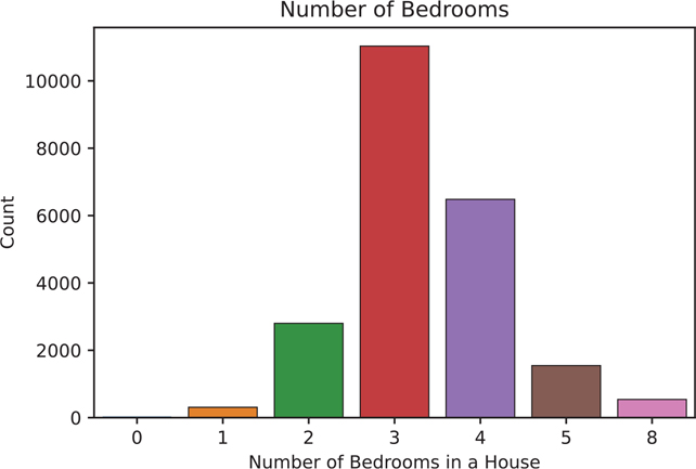
Figure 14.1 Bar plot using the statsmodels countplot() function of the NumBedrooms variable
import matplotlib.pyplot as plt

fig, ax = plt.subplots()
sns.countplot(data = acs, x = "NumBedrooms", ax=ax)

ax.set_title('Number of Bedrooms')
ax.set_xlabel('Number of Bedrooms in a House')
ax.set_ylabel('Count')

plt.show()model = smf.poisson(
"NumBedrooms ~ HouseCosts + OwnRent", data=acs
)
results = model.fit()
print(results.summary())Optimization terminated successfully.
Current function value: 1.680998
Iterations 10
Poisson Regression Results
==============================================================================
Dep. Variable: NumBedrooms No. Observations: 22745
Model: Poisson Df Residuals: 22741
Method: MLE Df Model: 3
Date: Thu, 01 Sep 2022 Pseudo R-squ.: 0.008309
Time: 01:55:49 Log-Likelihood: -38234.
converged: True LL-Null: -38555.
Covariance Type: nonrobust LLR p-value: 1.512e-138
======================================================================================
coef std err z P>|z| [0.025 0.975]
--------------------------------------------------------------------------------------
Intercept 1.1387 0.006 184.928 0.000 1.127 1.151
OwnRent[T.Outright] -0.2659 0.051 -5.182 0.000 -0.367 -0.165
OwnRent[T.Rented] -0.1237 0.012 -9.996 0.000 -0.148 -0.099
HouseCosts 6.217e-05 2.96e-06 21.017 0.000 5.64e-05 6.8e-05
======================================================================================The benefit of using a generalized linear model is that the only things that need to be changed are the family of the model that needs to be fit, and the link function that transforms our data. We can also use the more general glm() function to perform all the same calculations.
import statsmodels.api as sm
import statsmodels.formula.api as smf

model = smf.glm(
   "NumBedrooms ~ HouseCosts + OwnRent",
   data=acs,
   family=sm.families.Poisson(sm.genmod.families.links.log()),
).fit()
In this example, we are using the Poisson family, which comes from sm.families. Poisson, and we’re passing in the log link function via sm.genmod.families.links.log(). We get the same values as we did earlier when we use this method.
print(results.summary()) Poisson Regression Results
==============================================================================
Dep. Variable: NumBedrooms No. Observations: 22745
Model: Poisson Df Residuals: 22741
Method: MLE Df Model: 3
Date: Thu, 01 Sep 2022 Pseudo R-squ.: 0.008309
Time: 01:55:49 Log-Likelihood: -38234.
converged: True LL-Null: -38555.
Covariance Type: nonrobust LLR p-value: 1.512e-138
=====================================================================================
coef std err z P>|z| [0.025 0.975]
-------------------------------------------------------------------------------------
Intercept 1.1387 0.006 184.928 0.000 1.127 1.151
OwnRent[T.Outright] -0.2659 0.051 -5.182 0.000 -0.367 -0.165
OwnRent[T.Rented] -0.1237 0.012 -9.996 0.000 -0.148 -0.099
HouseCosts 6.217e-05 2.96e-06 21.017 0.000 5.64e-05 6.8e-05
=====================================================================================14.2.2 Negative Binomial Regression for Overdispersion
If our assumptions for Poisson regression are violated—that is, if our data has overdispersion—we can perform a negative binomial regression instead (Figure 14.2). Overdispersion is the statistics term meaning the numbers have more variance than expected, i.e., the values are too spread out.
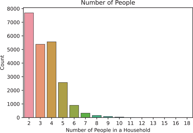
Figure 14.2 Bar plot using the statsmodels countplot() function of the NumPeople variable
fig, ax = plt.subplots()

sns.countplot(data = acs, x = "NumPeople", ax=ax)
ax.set_title('Number of People')
ax.set_xlabel('Number of People in a Household')
ax.set_ylabel('Count')

plt.show()model = smf.glm(
"NumPeople ~ Acres + NumVehicles",
data=acs,
family=sm.families.NegativeBinomial(
sm.genmod.families.links.log()
),
)
results = model.fit()print(results.summary()) Generalized Linear Model Regression Results
==============================================================================
Dep. Variable: NumPeople No. Observations: 22745
Model: GLM Df Residuals: 22741
Model Family: NegativeBinomial Df Model: 3
Link Function: log Scale: 1.0000
Method: IRLS Log-Likelihood: -53542.
Date: Thu, 01 Sep 2022 Deviance: 2605.6
Time: 01:55:50 Pearson chi2: 2.99e+03
No. Iterations: 6 Pseudo R-squ. (CS): 0.003504
Covariance Type: nonrobust
================================================================================
coef std err z P>|z| [0.025 0.975]
--------------------------------------------------------------------------------
Intercept 1.0418 0.025 41.580 0.000 0.993 1.091
Acres[T.10+] -0.0225 0.040 -0.564 0.573 -0.101 0.056
Acres[T.Sub 1] 0.0509 0.019 2.671 0.008 0.014 0.088
NumVehicles 0.0661 0.008 8.423 0.000 0.051 0.081
================================================================================Look for the reference variable in Acres.
print(acs["Acres"].value_counts())Sub 1 17114
1-10 4627
10+ 1004
Name: Acres, dtype: int6414.3 More Generalized Linear Models
The documentation page for GLM found in statsmodels lists the various families that can be passed into the glm parameter.1 These families can all be found under sm.families.<FAMILY>:
BinomialGammaGaussianInverseGaussianNegativeBinomialPoissonTweedie
The link functions are found under sm.families.family.<FAMILY>.links. Following is the list of link functions, but note that not all link functions are available for each family:
CDFLinkCLogLogLogLogLogLogitNegativeBinomialPowercauchycloglogloglogidentityinverse_powerinverse_squaredloglogit
For example, using the all the link functions for the Binomial family.
1. https://www.statsmodels.org/dev/glm.html
sm.families.family.Binomial.links[statsmodels.genmod.families.links.Logit,
statsmodels.genmod.families.links.probit,
statsmodels.genmod.families.links.cauchy,
statsmodels.genmod.families.links.Log,
statsmodels.genmod.families.links.CLogLog,
statsmodels.genmod.families.links.LogLog,
statsmodels.genmod.families.links.identity]Conclusion
This chapter covered some of the most basic and common models used in data analysis. These types of models serve as an interpretable baseline for more complex machine learning models. As we cover more complex models, keep in mind that sometimes simple and tried-and-true interpretable models can outperform the fancy newer models.