Chapter Objectives
After reading this chapter, you’ll be able to do the following:
• Clear the window to an arbitrary color
• Force any pending drawing to complete
• Draw with any geometric primitive—point, line, or polygon—in two or three dimensions
• Turn states on and off and query state variables
• Control the display of geometric primitives—for example, draw dashed lines or outlined polygons
• Specify normal vectors at appropriate points on the surfaces of solid objects
• Use vertex arrays and buffer objects to store and access geometric data with fewer function calls
• Save and restore several state variables at once
Although you can draw complex and interesting pictures using OpenGL, they’re all constructed from a small number of primitive graphical items. This shouldn’t be too surprising—look at what Leonardo da Vinci accomplished with just pencils and paintbrushes.
At the highest level of abstraction, there are three basic drawing operations: clearing the window, drawing a geometric object, and drawing a raster object. Raster objects, which include such things as two-dimensional images, bitmaps, and character fonts, are covered in Chapter 8. In this chapter, you learn how to clear the screen and draw geometric objects, including points, straight lines, and flat polygons.
You might think to yourself, “Wait a minute. I’ve seen lots of computer graphics in movies and on television, and there are plenty of beautifully shaded curved lines and surfaces. How are those drawn if OpenGL can draw only straight lines and flat polygons?” Even the image on the cover of this book includes a round table and objects on the table that have curved surfaces. It turns out that all the curved lines and surfaces you’ve seen are approximated by large numbers of little flat polygons or straight lines, in much the same way that the globe on the cover is constructed from a large set of rectangular blocks. The globe doesn’t appear to have a smooth surface because the blocks are relatively large compared with the globe. Later in this chapter, we show you how to construct curved lines and surfaces from lots of small geometric primitives.
This chapter has the following major sections:
• “A Drawing Survival Kit” explains how to clear the window and force drawing to be completed. It also gives you basic information about controlling the colors of geometric objects and describing a coordinate system.
• “Describing Points, Lines, and Polygons” shows you the set of primitive geometric objects and how to draw them.
• “Basic State Management” describes how to turn on and off some states (modes) and query state variables.
• “Displaying Points, Lines, and Polygons” explains what control you have over the details of how primitives are drawn—for example, what diameters points have, whether lines are solid or dashed, and whether polygons are outlined or filled.
• “Normal Vectors” discusses how to specify normal vectors for geometric objects and (briefly) what these vectors are for.
• “Vertex Arrays” shows you how to put large amounts of geometric data into just a few arrays and how, with only a few function calls, to render the geometry it describes. Reducing function calls may increase the efficiency and performance of rendering.
• “Buffer Objects” details how to use server-side memory buffers to store vertex array data for more efficient geometric rendering.
• “Vertex-Array Objects” expands the discussions of vertex arrays and buffer objects by describing how to efficiently change among sets of vertex arrays.
• “Attribute Groups” reveals how to query the current value of state variables and how to save and restore several related state values all at once.
• “Some Hints for Building Polygonal Models of Surfaces” explores the issues and techniques involved in constructing polygonal approximations to surfaces.
One thing to keep in mind as you read the rest of this chapter is that with OpenGL, unless you specify otherwise, every time you issue a drawing command, the specified object is drawn. This might seem obvious, but in some systems, you first make a list of things to draw. When your list is complete, you tell the graphics hardware to draw the items in the list. The first style is called immediate-mode graphics and is the default OpenGL style. In addition to using immediate mode, you can choose to save some commands in a list (called a display list) for later drawing. Immediate-mode graphics are typically easier to program, but display lists are often more efficient. Chapter 7 tells you how to use display lists and why you might want to use them.
Version 1.1 of OpenGL introduced vertex arrays.
In Version 1.2, scaling of surface normals (GL_RESCALE_NORMAL) was added to OpenGL. Also, glDrawRangeElements() supplemented vertex arrays.
Version 1.3 marked the initial support for texture coordinates for multiple texture units in the OpenGL core feature set. Previously, multitexturing had been an optional OpenGL extension.
In Version 1.4, fog coordinates and secondary colors may be stored in vertex arrays, and the commands glMultiDrawArrays() and glMultiDrawElements() may be used to render primitives from vertex arrays.
In Version 1.5, vertex arrays may be stored in buffer objects that may be able to use server memory for storing arrays and potentially accelerating their rendering.
Version 3.0 added support for vertex array objects, allowing all of the state related to vertex arrays to be bundled and activated with a single call. This, in turn, makes switching between sets of vertex arrays simpler and faster.
Version 3.1 removed most of the immediate-mode routines and added the primitive restart index, which allows you to render multiple primitives (of the same type) with a single drawing call.
This section explains how to clear the window in preparation for drawing, set the colors of objects that are to be drawn, and force drawing to be completed. None of these subjects has anything to do with geometric objects in a direct way, but any program that draws geometric objects has to deal with these issues.
Drawing on a computer screen is different from drawing on paper in that the paper starts out white, and all you have to do is draw the picture. On a computer, the memory holding the picture is usually filled with the last picture you drew, so you typically need to clear it to some background color before you start to draw the new scene. The color you use for the background depends on the application. For a word processor, you might clear to white (the color of the paper) before you begin to draw the text. If you’re drawing a view from a spaceship, you clear to the black of space before beginning to draw the stars, planets, and alien spaceships. Sometimes you might not need to clear the screen at all; for example, if the image is the inside of a room, the entire graphics window is covered as you draw all the walls.
At this point, you might be wondering why we keep talking about clearing the window—why not just draw a rectangle of the appropriate color that’s large enough to cover the entire window? First, a special command to clear a window can be much more efficient than a general-purpose drawing command. In addition, as you’ll see in Chapter 3, OpenGL allows you to set the coordinate system, viewing position, and viewing direction arbitrarily, so it might be difficult to figure out an appropriate size and location for a window-clearing rectangle. Finally, on many machines, the graphics hardware consists of multiple buffers in addition to the buffer containing colors of the pixels that are displayed. These other buffers must be cleared from time to time, and it’s convenient to have a single command that can clear any combination of them. (See Chapter 10 for a discussion of all the possible buffers.)
You must also know how the colors of pixels are stored in the graphics hardware known as bitplanes. There are two methods of storage. Either the red, green, blue, and alpha (RGBA) values of a pixel can be directly stored in the bitplanes, or a single index value that references a color lookup table is stored. RGBA color-display mode is more commonly used, so most of the examples in this book use it. (See Chapter 4 for more information about both display modes.) You can safely ignore all references to alpha values until Chapter 6.
As an example, these lines of code clear an RGBA mode window to black:
glClearColor(0.0, 0.0, 0.0, 0.0);
glClear(GL_COLOR_BUFFER_BIT);
The first line sets the clearing color to black, and the next command clears the entire window to the current clearing color. The single parameter to glClear() indicates which buffers are to be cleared. In this case, the program clears only the color buffer, where the image displayed on the screen is kept. Typically, you set the clearing color once, early in your application, and then you clear the buffers as often as necessary. OpenGL keeps track of the current clearing color as a state variable, rather than requiring you to specify it each time a buffer is cleared.
Chapter 4 and Chapter 10 discuss how other buffers are used. For now, all you need to know is that clearing them is simple. For example, to clear both the color buffer and the depth buffer, you would use the following sequence of commands:
glClearColor(0.0, 0.0, 0.0, 0.0);
glClearDepth(1.0);
glClear(GL_COLOR_BUFFER_BIT | GL_DEPTH_BUFFER_BIT);
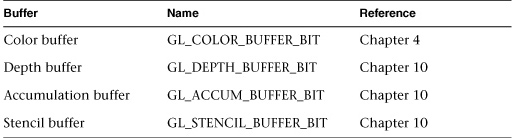
In this case, the call to glClearColor() is the same as before, the glClearDepth() command specifies the value to which every pixel of the depth buffer is to be set, and the parameter to the glClear() command now consists of the bitwise logical OR of all the buffers to be cleared. The following summary of glClear() includes a table that lists the buffers that can be cleared, their names, and the chapter in which each type of buffer is discussed.
|
Compatibility Extension |
|
GL_ACCUM_BUFFER_BIT |
Before issuing a command to clear multiple buffers, you have to set the values to which each buffer is to be cleared if you want something other than the default RGBA color, depth value, accumulation color, and stencil index. In addition to the glClearColor() and glClearDepth() commands that set the current values for clearing the color and depth buffers, glClearIndex(), glClearAccum(), and glClearStencil() specify the color index, accumulation color, and stencil index used to clear the corresponding buffers. (See Chapter 4 and Chapter 10 for descriptions of these buffers and their uses.)
OpenGL allows you to specify multiple buffers because clearing is generally a slow operation, as every pixel in the window (possibly millions) is touched, and some graphics hardware allows sets of buffers to be cleared simultaneously. Hardware that doesn’t support simultaneous clears performs them sequentially. The difference between
glClear(GL_COLOR_BUFFER_BIT | GL_DEPTH_BUFFER_BIT);
glClear(GL_COLOR_BUFFER_BIT);
glClear(GL_DEPTH_BUFFER_BIT);
is that although both have the same final effect, the first example might run faster on many machines. It certainly won’t run more slowly.
With OpenGL, the description of the shape of an object being drawn is independent of the description of its color. Whenever a particular geometric object is drawn, it’s drawn using the currently specified coloring scheme. The coloring scheme might be as simple as “draw everything in fire-engine red” or as complicated as “assume the object is made out of blue plastic, that there’s a yellow spotlight pointed in such and such a direction, and that there’s a general low-level reddish-brown light everywhere else.” In general, an OpenGL programmer first sets the color or coloring scheme and then draws the objects. Until the color or coloring scheme is changed, all objects are drawn in that color or using that coloring scheme. This method helps OpenGL achieve higher drawing performance than would result if it didn’t keep track of the current color.
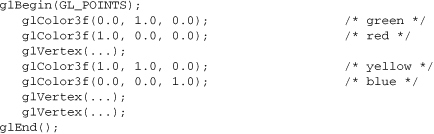
For example, the pseudocode
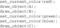
draws objects A and B in red, and object C in blue. The command on the fourth line that sets the current color to green is wasted.
Coloring, lighting, and shading are all large topics with entire chapters or large sections devoted to them. To draw geometric primitives that can be seen, however, you need some basic knowledge of how to set the current color; this information is provided in the next few paragraphs. (See Chapter 4 and Chapter 5 for details on these topics.)
To set a color, use the command glColor3f(). It takes three parameters, all of which are floating-point numbers between 0.0 and 1.0. The parameters are, in order, the red, green, and blue components of the color. You can think of these three values as specifying a “mix” of colors: 0.0 means don’t use any of that component, and 1.0 means use all you can of that component. Thus, the code
glColor3f(1.0, 0.0, 0.0);
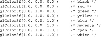
makes the brightest red the system can draw, with no green or blue components. All zeros makes black; in contrast, all ones makes white. Setting all three components to 0.5 yields gray (halfway between black and white). Here are eight commands and the colors they would set:
You might have noticed earlier that the routine for setting the clearing color, glClearColor(), takes four parameters, the first three of which match the parameters for glColor3f(). The fourth parameter is the alpha value; it’s covered in detail in “Blending” in Chapter 6. For now, set the fourth parameter of glClearColor() to 0.0, which is its default value.
As you saw in “OpenGL Rendering Pipeline” in Chapter 1, most modern graphics systems can be thought of as an assembly line. The main central processing unit (CPU) issues a drawing command. Perhaps other hardware does geometric transformations. Clipping is performed, followed by shading and/or texturing. Finally, the values are written into the bitplanes for display. In high-end architectures, each of these operations is performed by a different piece of hardware that’s been designed to perform its particular task quickly. In such an architecture, there’s no need for the CPU to wait for each drawing command to complete before issuing the next one. While the CPU is sending a vertex down the pipeline, the transformation hardware is working on transforming the last one sent, the one before that is being clipped, and so on. In such a system, if the CPU waited for each command to complete before issuing the next, there could be a huge performance penalty.
In addition, the application might be running on more than one machine. For example, suppose that the main program is running elsewhere (on a machine called the client) and that you’re viewing the results of the drawing on your workstation or terminal (the server), which is connected by a network to the client. In that case, it might be horribly inefficient to send each command over the network one at a time, as considerable overhead is often associated with each network transmission. Usually, the client gathers a collection of commands into a single network packet before sending it. Unfortunately, the network code on the client typically has no way of knowing that the graphics program is finished drawing a frame or scene. In the worst case, it waits forever for enough additional drawing commands to fill a packet, and you never see the completed drawing.
For this reason, OpenGL provides the command glFlush(), which forces the client to send the network packet even though it might not be full. Where there is no network and all commands are truly executed immediately on the server, glFlush() might have no effect. However, if you’re writing a program that you want to work properly both with and without a network, include a call to glFlush() at the end of each frame or scene. Note that glFlush() doesn’t wait for the drawing to complete—it just forces the drawing to begin execution, thereby guaranteeing that all previous commands execute in finite time even if no further rendering commands are executed.
There are other situations in which glFlush() is useful:
• Software renderers that build images in system memory and don’t want to constantly update the screen.
• Implementations that gather sets of rendering commands to amortize start-up costs. The aforementioned network transmission example is one instance of this.
Whenever you initially open a window or later move or resize that window, the window system will send an event to notify you. If you are using GLUT, the notification is automated; whatever routine has been registered to glutReshapeFunc() will be called. You must register a callback function that will
• Reestablish the rectangular region that will be the new rendering canvas
• Define the coordinate system to which objects will be drawn
In Chapter 3, you’ll see how to define three-dimensional coordinate systems, but right now just create a simple, basic two-dimensional coordinate system into which you can draw a few objects. Call glutReshapeFunc(reshape), where reshape() is the following function shown in Example 2-1.
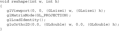
The kernel of GLUT will pass this function two arguments: the width and height, in pixels, of the new, moved, or resized window. glViewport() adjusts the pixel rectangle for drawing to be the entire new window. The next three routines adjust the coordinate system for drawing so that the lower left corner is (0, 0) and the upper right corner is (w, h) (see Figure 2-1).
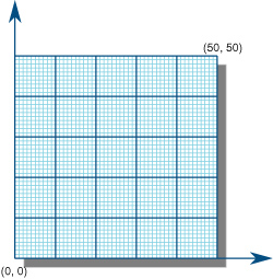
To explain it another way, think about a piece of graphing paper. The w and h values in reshape() represent how many columns and rows of squares are on your graph paper. Then you have to put axes on the graph paper. The gluOrtho2D() routine puts the origin, (0, 0), in the lowest, leftmost square, and makes each square represent one unit. Now, when you render the points, lines, and polygons in the rest of this chapter, they will appear on this paper in easily predictable squares. (For now, keep all your objects two-dimensional.)
This section explains how to describe OpenGL geometric primitives. All geometric primitives are eventually described in terms of their vertices—coordinates that define the points themselves, the endpoints of line segments, or the corners of polygons. The next section discusses how these primitives are displayed and what control you have over their display.
You probably have a fairly good idea of what a mathematician means by the terms point, line, and polygon. The OpenGL meanings are similar, but not quite the same.
One difference comes from the limitations of computer-based calculations. In any OpenGL implementation, floating-point calculations are of finite precision, and they have round-off errors. Consequently, the coordinates of OpenGL points, lines, and polygons suffer from the same problems.
A more important difference arises from the limitations of a raster graphics display. On such a display, the smallest displayable unit is a pixel, and although pixels might be less than 1/100 of an inch wide, they are still much larger than the mathematician’s concepts of infinitely small (for points) and infinitely thin (for lines). When OpenGL performs calculations, it assumes that points are represented as vectors of floating-point numbers. However, a point is typically (but not always) drawn as a single pixel, and many different points with slightly different coordinates could be drawn by OpenGL on the same pixel.
A point is represented by a set of floating-point numbers called a vertex. All internal calculations are done as if vertices are three-dimensional. Vertices specified by the user as two-dimensional (that is, with only x- and y-coordinates) are assigned a z-coordinate equal to zero by OpenGL.
Advanced
OpenGL works in the homogeneous coordinates of three-dimensional projective geometry, so for internal calculations, all vertices are represented with four floating-point coordinates (x, y, z, w). If w is different from zero, these coordinates correspond to the Euclidean, three-dimensional point (x/w, y/w, z/w). You can specify the w-coordinate in OpenGL commands, but this is rarely done. If the w-coordinate isn’t specified, it is understood to be 1.0. (See Appendix C for more information about homogeneous coordinate systems.)
In OpenGL, the term line refers to a line segment, not the mathematician’s version that extends to infinity in both directions. There are easy ways to specify a connected series of line segments, or even a closed, connected series of segments (see Figure 2-2). In all cases, though, the lines constituting the connected series are specified in terms of the vertices at their endpoints.
Polygons are the areas enclosed by single closed loops of line segments, where the line segments are specified by the vertices at their endpoints. Polygons are typically drawn with the pixels in the interior filled in, but you can also draw them as outlines or a set of points. (See “Polygon Details” on page 60.)
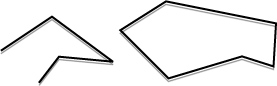
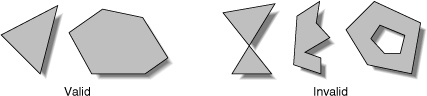
In general, polygons can be complicated, so OpenGL imposes some strong restrictions on what constitutes a primitive polygon. First, the edges of OpenGL polygons can’t intersect (a mathematician would call a polygon satisfying this condition a simple polygon). Second, OpenGL polygons must be convex, meaning that they cannot have indentations. Stated precisely, a region is convex if, given any two points in the interior, the line segment joining them is also in the interior. See Figure 2-3 for some examples of valid and invalid polygons. OpenGL, however, doesn’t restrict the number of line segments making up the boundary of a convex polygon. Note that polygons with holes can’t be described. They are nonconvex, and they can’t be drawn with a boundary made up of a single closed loop. Be aware that if you present OpenGL with a nonconvex filled polygon, it might not draw it as you expect. For instance, on most systems, no more than the convex hull of the polygon would be filled. On some systems, less than the convex hull might be filled.
The reason for the OpenGL restrictions on valid polygon types is that it’s simpler to provide fast polygon-rendering hardware for that restricted class of polygons. Simple polygons can be rendered quickly. The difficult cases are hard to detect quickly, so for maximum performance, OpenGL crosses its fingers and assumes the polygons are simple.
Many real-world surfaces consist of nonsimple polygons, nonconvex polygons, or polygons with holes. Since all such polygons can be formed from unions of simple convex polygons, some routines to build more complex objects are provided in the GLU library. These routines take complex descriptions and tessellate them, or break them down into groups of the simpler OpenGL polygons that can then be rendered. (See “Polygon Tessellation” in Chapter 11 for more information about the tessellation routines.)
Since OpenGL vertices are always three-dimensional, the points forming the boundary of a particular polygon don’t necessarily lie on the same plane in space. (Of course, they do in many cases—if all the z-coordinates are zero, for example, or if the polygon is a triangle.) If a polygon’s vertices don’t lie in the same plane, then after various rotations in space, changes in the viewpoint, and projection onto the display screen, the points might no longer form a simple convex polygon. For example, imagine a four-point quadrilateral where the points are slightly out of plane, and look at it almost edge-on. You can get a nonsimple polygon that resembles a bow tie, as shown in Figure 2-4, which isn’t guaranteed to be rendered correctly. This situation isn’t all that unusual if you approximate curved surfaces by quadrilaterals made of points lying on the true surface. You can always avoid the problem by using triangles, as any three points always lie on a plane.
Since rectangles are so common in graphics applications, OpenGL provides a filled-rectangle drawing primitive, glRect*(). You can draw a rectangle as a polygon, as described in “OpenGL Geometric Drawing Primitives” on page 47, but your particular implementation of OpenGL might have optimized glRect*() for rectangles.
|
Compatibility Extension |
|
glRect |
Note that although the rectangle begins with a particular orientation in three-dimensional space (in the xy-plane and parallel to the axes), you can change this by applying rotations or other transformations. (See Chapter 3 for information about how to do this.)
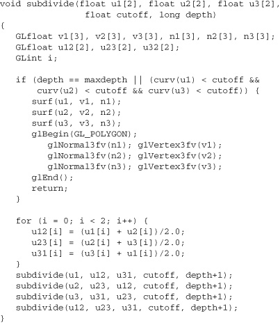
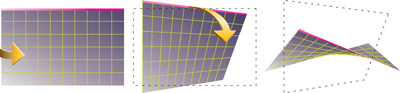
Any smoothly curved line or surface can be approximated—to any arbitrary degree of accuracy—by short line segments or small polygonal regions. Thus, subdividing curved lines and surfaces sufficiently and then approximating them with straight line segments or flat polygons makes them appear curved (see Figure 2-5). If you’re skeptical that this really works, imagine subdividing until each line segment or polygon is so tiny that it’s smaller than a pixel on the screen.
Even though curves aren’t geometric primitives, OpenGL provides some direct support for subdividing and drawing them. (See Chapter 12 for information about how to draw curves and curved surfaces.)
With OpenGL, every geometric object is ultimately described as an ordered set of vertices. You use the glVertex*() command to specify a vertex.
|
Compatibility Extension |
|
glVertex |
Example 2-2 provides some examples of using glVertex*().
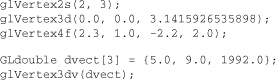
The first example represents a vertex with three-dimensional coordinates (2, 3, 0). (Remember that if it isn’t specified, the z-coordinate is understood to be 0.) The coordinates in the second example are (0.0, 0.0, 3.1415926535898) (double-precision floating-point numbers). The third example represents the vertex with three-dimensional coordinates (1.15, 0.5, −1.1) as a homogenous coordinate. (Remember that the x-, y-, and z-coordinates are eventually divided by the w-coordinate.) In the final example, dvect is a pointer to an array of three double-precision floating-point numbers.
On some machines, the vector form of glVertex*() is more efficient, since only a single parameter needs to be passed to the graphics subsystem. Special hardware might be able to send a whole series of coordinates in a single batch. If your machine is like this, it’s to your advantage to arrange your data so that the vertex coordinates are packed sequentially in memory. In this case, there may be some gain in performance by using the vertex array operations of OpenGL. (See “Vertex Arrays” on page 70.)
Now that you’ve seen how to specify vertices, you still need to know how to tell OpenGL to create a set of points, a line, or a polygon from those vertices. To do this, you bracket each set of vertices between a call to glBegin() and a call to glEnd(). The argument passed to glBegin() determines what sort of geometric primitive is constructed from the vertices. For instance, Example 2-3 specifies the vertices for the polygon shown in Figure 2-6.
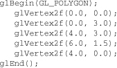

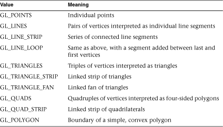
If you had used GL_POINTS instead of GL_POLYGON, the primitive would have been simply the five points shown in Figure 2-6. Table 2-2 in the following function summary for glBegin() lists the 10 possible arguments and the corresponding types of primitives.
|
Compatibility Extension |
|
glBegin GL_QUADS GL_QUAD_STRIP GL_POLYGON |
|
Compatibility Extension |
|
glEnd |
Figure 2-7 shows examples of all the geometric primitives listed in Table 2-2, with descriptions of the pixels that are drawn for each of the objects. Note that in addition to points, several types of lines and polygons are defined. Obviously, you can find many ways to draw the same primitive. The method you choose depends on your vertex data.
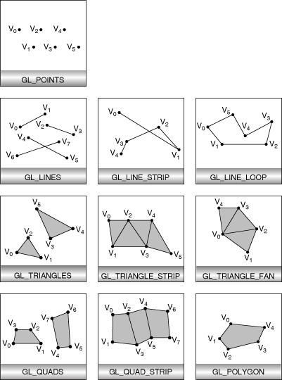
As you read the following descriptions, assume that n vertices (v0, v1, v2, ..., vn–1) are described between a glBegin() and glEnd() pair.


The most important information about vertices is their coordinates, which are specified by the glVertex*() command. You can also supply additional vertex-specific data for each vertex—a color, a normal vector, texture coordinates, or any combination of these—using special commands. In addition, a few other commands are valid between a glBegin() and glEnd() pair. Table 2-3 contains a complete list of such valid commands.

No other OpenGL commands are valid between a glBegin() and glEnd() pair, and making most other OpenGL calls generates an error. Some vertex array commands, such as glEnableClientState() and glVertexPointer(), when called between glBegin() and glEnd(), have undefined behavior but do not necessarily generate an error. (Also, routines related to OpenGL, such as glX*() routines, have undefined behavior between glBegin() and glEnd().) These cases should be avoided, and debugging them may be more difficult.
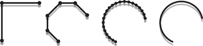
Note, however, that only OpenGL commands are restricted; you can certainly include other programming-language constructs (except for calls, such as the aforementioned glX*() routines). For instance, Example 2-4 draws an outlined circle.
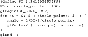
Note
This example isn’t the most efficient way to draw a circle, especially if you intend to do it repeatedly. The graphics commands used are typically very fast, but this code calculates an angle and calls the sin() and cos() routines for each vertex; in addition, there’s the loop overhead. (Another way to calculate the vertices of a circle is to use a GLU routine; see “Quadrics: Rendering Spheres, Cylinders, and Disks” in Chapter 11.) If you need to draw numerous circles, calculate the coordinates of the vertices once and save them in an array and create a display list (see Chapter 7), or use vertex arrays to render them.
Unless they are being compiled into a display list, all glVertex*() commands should appear between a glBegin() and glEnd() combination. (If they appear elsewhere, they don’t accomplish anything.) If they appear in a display list, they are executed only if they appear between a glBegin() and a glEnd(). (See Chapter 7 for more information about display lists.)
Although many commands are allowed between glBegin() and glEnd(), vertices are generated only when a glVertex*() command is issued. At the moment glVertex*() is called, OpenGL assigns the resulting vertex the current color, texture coordinates, normal vector information, and so on. To see this, look at the following code sequence. The first point is drawn in red, and the second and third ones in blue, despite the extra color commands:
You can use any combination of the 24 versions of the glVertex*() command between glBegin() and glEnd(), although in real applications all the calls in any particular instance tend to be of the same form. If your vertex-data specification is consistent and repetitive (for example, glColor*, glVertex*, glColor*, glVertex*,...), you may enhance your program’s performance by using vertex arrays. (See “Vertex Arrays” on page 70.)
In the preceding section, you saw an example of a state variable, the current RGBA color, and how it can be associated with a primitive. OpenGL maintains many states and state variables. An object may be rendered with lighting, texturing, hidden surface removal, fog, and other states affecting its appearance.
By default, most of these states are initially inactive. These states may be costly to activate; for example, turning on texture mapping will almost certainly slow down the process of rendering a primitive. However, the image will improve in quality and will look more realistic, owing to the enhanced graphics capabilities.
To turn many of these states on and off, use these two simple commands:
You can also check whether a state is currently enabled or disabled.
The states you have just seen have two settings: on and off. However, most OpenGL routines set values for more complicated state variables. For example, the routine glColor3f() sets three values, which are part of the GL_CURRENT_COLOR state. There are five querying routines used to find out what values are set for many states:
These querying routines handle most, but not all, requests for obtaining state information. (See “The Query Commands” in Appendix B for a list of all of the available OpenGL state querying routines.)
By default, a point is drawn as a single pixel on the screen, a line is drawn solid and 1 pixel wide, and polygons are drawn solidly filled in. The following paragraphs discuss the details of how to change these default display modes.
To control the size of a rendered point, use glPointSize() and supply the desired size in pixels as the argument.
The actual collection of pixels on the screen that are drawn for various point widths depends on whether antialiasing is enabled. (Antialiasing is a technique for smoothing points and lines as they’re rendered; see “Antialiasing” and “Point Parameters” in Chapter 6 for more detail.) If antialiasing is disabled (the default), fractional widths are rounded to integer widths, and a screen-aligned square region of pixels is drawn. Thus, if the width is 1.0, the square is 1 pixel by 1 pixel; if the width is 2.0, the square is 2 pixels by 2 pixels; and so on.
With antialiasing or multisampling enabled, a circular group of pixels is drawn, and the pixels on the boundaries are typically drawn at less than full intensity to give the edge a smoother appearance. In this mode, noninteger widths aren’t rounded.
Most OpenGL implementations support very large point sizes. You can query the minimum and maximum sized for aliased points by using GL_ALIASED_POINT_SIZE_RANGE with glGetFloatv(). Likewise, you can obtain the range of supported sizes for antialiased points by passing GL_SMOOTH_POINT_SIZE_RANGE to glGetFloatv(). The sizes of supported antialiased points are evenly spaced between the minimum and maximum sizes for the range. Calling glGetFloatv() with the parameter GL_SMOOTH_POINT_SIZE_GRANULARITY will return how accurately a given antialiased point size is supported. For example, if you request glPointSize(2.37) and the granularity returned is 0.1, then the point size is rounded to 2.4.
With OpenGL, you can specify lines with different widths and lines that are stippled in various ways—dotted, dashed, drawn with alternating dots and dashes, and so on.
The actual rendering of lines is affected if either antialiasing or multisampling is enabled. (See “Antialiasing Points or Lines” on page 269 and “Antialiasing Geometric Primitives with Multisampling” on page 275.) Without antialiasing, widths of 1, 2, and 3 draw lines 1, 2, and 3 pixels wide. With antialiasing enabled, noninteger line widths are possible, and pixels on the boundaries are typically drawn at less than full intensity. As with point sizes, a particular OpenGL implementation might limit the width of nonantialiased lines to its maximum antialiased line width, rounded to the nearest integer value. You can obtain the range of supported aliased line widths by using GL_ALIASED_LINE_WIDTH_RANGE with glGetFloatv(). To determine the supported minimum and maximum sizes of antialiased line widths, and what granularity your implementation supports, call glGetFloatv(), with GL_SMOOTH_LINE_WIDTH_RANGE and GL_SMOOTH_LINE_WIDTH_GRANULARITY.
Note
Keep in mind that, by default, lines are 1 pixel wide, so they appear wider on lower-resolution screens. For computer displays, this isn’t typically an issue, but if you’re using OpenGL to render to a high-resolution plotter, 1-pixel lines might be nearly invisible. To obtain resolution-independent line widths, you need to take into account the physical dimensions of pixels.
Advanced
With non-antialiased wide lines, the line width isn’t measured perpendicular to the line. Instead, it’s measured in the y-direction if the absolute value of the slope is less than 1.0; otherwise, it’s measured in the x-direction. The rendering of an antialiased line is exactly equivalent to the rendering of a filled rectangle of the given width, centered on the exact line.
To make stippled (dotted or dashed) lines, you use the command glLineStipple() to define the stipple pattern, and then you enable line stippling with glEnable().
glLineStipple(1, 0x3F07);
glEnable(GL_LINE_STIPPLE);
|
Compatibility Extension |
|
glLineStipple GL_LINE_STIPPLE |
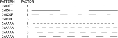
With the preceding example and the pattern 0X3F07 (which translates to 0011111100000111 in binary), a line would be drawn with 3 pixels on, then 5 off, 6 on, and 2 off. (If this seems backward, remember that the low-order bit is used first.) If factor had been 2, the pattern would have been elongated: 6 pixels on, 10 off, 12 on, and 4 off. Figure 2-8 shows lines drawn with different patterns and repeat factors. If you don’t enable line stippling, drawing proceeds as if pattern were 0xFFFF and factor were 1. (Use glDisable() with GL_LINE_STIPPLE to disable stippling.) Note that stippling can be used in combination with wide lines to produce wide stippled lines.
One way to think of the stippling is that as the line is being drawn, the pattern is shifted by 1 bit each time a pixel is drawn (or factor pixels are drawn, if factor isn’t 1). When a series of connected line segments is drawn between a single glBegin() and glEnd(), the pattern continues to shift as one segment turns into the next. This way, a stippling pattern continues across a series of connected line segments. When glEnd() is executed, the pattern is reset, and if more lines are drawn before stippling is disabled the stippling restarts at the beginning of the pattern. If you’re drawing lines with GL_LINES, the pattern resets for each independent line.
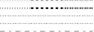
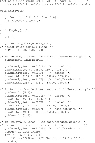
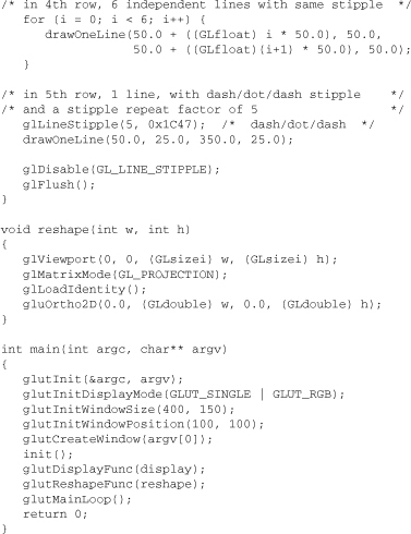
Example 2-5 illustrates the results of drawing with a couple of different stipple patterns and line widths. It also illustrates what happens if the lines are drawn as a series of individual segments instead of a single connected line strip. The results of running the program appear in Figure 2-9.
Polygons are typically drawn by filling in all the pixels enclosed within the boundary, but you can also draw them as outlined polygons or simply as points at the vertices. A filled polygon might be solidly filled or stippled with a certain pattern. Although the exact details are omitted here, filled polygons are drawn in such a way that if adjacent polygons share an edge or vertex, the pixels making up the edge or vertex are drawn exactly once—they’re included in only one of the polygons. This is done so that partially transparent polygons don’t have their edges drawn twice, which would make those edges appear darker (or brighter, depending on what color you’re drawing with). Note that it might result in narrow polygons having no filled pixels in one or more rows or columns of pixels.
To antialias filled polygons, multisampling is highly recommended. For details, see “Antialiasing Geometric Primitives with Multisampling” in Chapter 6.
A polygon has two sides—front and back—and might be rendered differently depending on which side is facing the viewer. This allows you to have cutaway views of solid objects in which there is an obvious distinction between the parts that are inside and those that are outside. By default, both front and back faces are drawn in the same way. To change this, or to draw only outlines or vertices, use glPolygonMode().
|
Compatibility Extension |
|
GL_FRONT GL_BACK |
For example, you can have the front faces filled and the back faces outlined with two calls to this routine:
glPolygonMode(GL_FRONT, GL_FILL);
glPolygonMode(GL_BACK, GL_LINE);
By convention, polygons whose vertices appear in counterclockwise order on the screen are called front-facing. You can construct the surface of any “reasonable” solid—a mathematician would call such a surface an orientable manifold (spheres, donuts, and teapots are orientable; Klein bottles and Möbius strips aren’t)—from polygons of consistent orientation. In other words, you can use all clockwise polygons or all counterclockwise polygons. (This is essentially the mathematical definition of orientable.)
Suppose you’ve consistently described a model of an orientable surface but happen to have the clockwise orientation on the outside. You can swap what OpenGL considers the back face by using the function glFrontFace(), supplying the desired orientation for front-facing polygons.
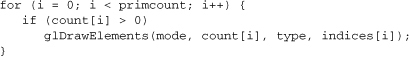
In a completely enclosed surface constructed from opaque polygons with a consistent orientation, none of the back-facing polygons are ever visible—they’re always obscured by the front-facing polygons. If you are outside this surface, you might enable culling to discard polygons that OpenGL determines are back-facing. Similarly, if you are inside the object, only back-facing polygons are visible. To instruct OpenGL to discard front- or back-facing polygons, use the command glCullFace() and enable culling with glEnable().
Advanced
In more technical terms, deciding whether a face of a polygon is front-or back-facing depends on the sign of the polygon’s area computed in window coordinates. One way to compute this area is
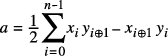
where xi and yi are the x and y window coordinates of the ith vertex of the n-vertex polygon and
|
i⊕1 is (i+1) mod n. |
Assuming that GL_CCW has been specified, if a > 0, the polygon corresponding to that vertex is considered to be front-facing; otherwise, it’s back-facing. If GL_CW is specified and if a < 0, then the corresponding polygon is front-facing; otherwise, it’s back-facing.
Modify Example 2-5 by adding some filled polygons. Experiment with different colors. Try different polygon modes. Also, enable culling to see its effect.
By default, filled polygons are drawn with a solid pattern. They can also be filled with a 32-bit by 32-bit window-aligned stipple pattern, which you specify with glPolygonStipple().
|
Compatibility Extension |
|
glPolygonStipple GL_POLYGON_STIPPLE |
In addition to defining the current polygon stippling pattern, you must enable stippling:
glEnable(GL_POLYGON_STIPPLE);
Use glDisable() with the same argument to disable polygon stippling.
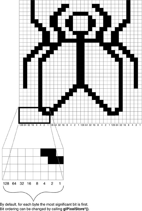
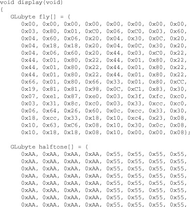
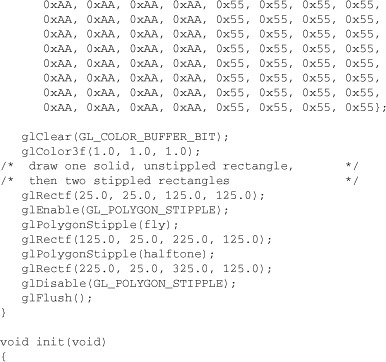
Figure 2-11 shows the results of polygons drawn unstippled and then with two different stippling patterns. The program is shown in Example 2-6. The reversal of white to black (from Figure 2-10 to Figure 2-11) occurs because the program draws in white over a black background, using the pattern in Figure 2-10 as a stencil.

You might want to use display lists to store polygon stipple patterns to maximize efficiency. (See “Display List Design Philosophy” in Chapter 7.)
Advanced
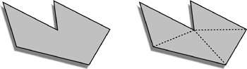
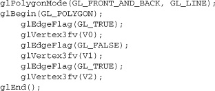
OpenGL can render only convex polygons, but many nonconvex polygons arise in practice. To draw these nonconvex polygons, you typically subdivide them into convex polygons—usually triangles, as shown in Figure 2-12—and then draw the triangles. Unfortunately, if you decompose a general polygon into triangles and draw the triangles, you can’t really use glPolygonMode() to draw the polygon’s outline, as you get all the triangle outlines inside it. To solve this problem, you can tell OpenGL whether a particular vertex precedes a boundary edge; OpenGL keeps track of this information by passing along with each vertex a bit indicating whether that vertex is followed by a boundary edge. Then, when a polygon is drawn in GL_LINE mode, the nonboundary edges aren’t drawn. In Figure 2-12, the dashed lines represent added edges.
By default, all vertices are marked as preceding a boundary edge, but you can manually control the setting of the edge flag with the command glEdgeFlag*(). This command is used between glBegin() and glEnd() pairs, and it affects all the vertices specified after it until the next glEdgeFlag() call is made. It applies only to vertices specified for polygons, triangles, and quads, not to those specified for strips of triangles or quads.
|
Compatibility Extension |
|
glEdgeFlag |
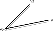
For instance, Example 2-7 draws the outline shown in Figure 2-13.
A normal vector (or normal, for short) is a vector that points in a direction that’s perpendicular to a surface. For a flat surface, one perpendicular direction is the same for every point on the surface, but for a general curved surface, the normal direction might be different at each point on the surface. With OpenGL, you can specify a normal for each polygon or for each vertex. Vertices of the same polygon might share the same normal (for a flat surface) or have different normals (for a curved surface). You can’t assign normals anywhere other than at the vertices.
An object’s normal vectors define the orientation of its surface in space—in particular, its orientation relative to light sources. These vectors are used by OpenGL to determine how much light the object receives at its vertices. Lighting—a large topic by itself—is the subject of Chapter 5, and you might want to review the following information after you’ve read that chapter. Normal vectors are discussed briefly here because you define normal vectors for an object at the same time you define the object’s geometry.
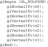
You use glNormal*() to set the current normal to the value of the argument passed in. Subsequent calls to glVertex*() cause the specified vertices to be assigned the current normal. Often, each vertex has a different normal, which necessitates a series of alternating calls, as in Example 2-8.
|
Compatibility Extension |
|
glNormal |
There’s no magic to finding the normals for an object—most likely, you have to perform some calculations that might include taking derivatives—but there are several techniques and tricks you can use to achieve certain effects. Appendix H, “Calculating Normal Vectors,”[1] explains how to find normal vectors for surfaces. If you already know how to do this, if you can count on always being supplied with normal vectors, or if you don’t want to use the OpenGL lighting facilities, you don’t need to read this appendix.
[1] This appendix is available online at http://www.opengl-redbook.com/appendices/.
Note that at a given point on a surface, two vectors are perpendicular to the surface, and they point in opposite directions. By convention, the normal is the one that points to the outside of the surface being modeled. (If you get inside and outside reversed in your model, just change every normal vector from (x, y, z) to (−x, −y, −z)).
Also, keep in mind that since normal vectors indicate direction only, their lengths are mostly irrelevant. You can specify normals of any length, but eventually they have to be converted to a length of 1 before lighting calculations are performed. (A vector that has a length of 1 is said to be of unit length, or normalized.) In general, you should supply normalized normal vectors. To make a normal vector of unit length, divide each of its x-, y-, z-components by the length of the normal:
Normal vectors remain normalized as long as your model transformations include only rotations and translations. (See Chapter 3 for a discussion of transformations.) If you perform irregular transformations (such as scaling or multiplying by a shear matrix), or if you specify nonunit-length normals, then you should have OpenGL automatically normalize your normal vectors after the transformations. To do this, call glEnable(GL_NORMALIZE).
|
Compatibility Extension |
|
GL_NORMALIZE GL_RESCALE_NORMAL |
If you supply unit-length normals, and you perform only uniform scaling (that is, the same scaling value for x, y, and z), you can use glEnable(GL_RESCALE_NORMAL) to scale the normals by a constant factor, derived from the modelview transformation matrix, to return them to unit length after transformation.
Note that automatic normalization or rescaling typically requires additional calculations that might reduce the performance of your application. Rescaling normals uniformly with GL_RESCALE_NORMAL is usually less expensive than performing full-fledged normalization with GL_NORMALIZE. By default, both automatic normalizing and rescaling operations are disabled.
You may have noticed that OpenGL requires many function calls to render geometric primitives. Drawing a 20-sided polygon requires at least 22 function calls: one call to glBegin(), one call for each of the vertices, and a final call to glEnd(). In the two previous code examples, additional information (polygon boundary edge flags or surface normals) added function calls for each vertex. This can quickly double or triple the number of function calls required for one geometric object. For some systems, function calls have a great deal of overhead and can hinder performance.
An additional problem is the redundant processing of vertices that are shared between adjacent polygons. For example, the cube in Figure 2-14 has six faces and eight shared vertices. Unfortunately, if the standard method of describing this object is used, each vertex has to be specified three times: once for every face that uses it. Therefore, 24 vertices are processed, even though eight would be enough.

OpenGL has vertex array routines that allow you to specify a lot of vertex-related data with just a few arrays and to access that data with equally few function calls. Using vertex array routines, all 20 vertices in a 20-sided polygon can be put into one array and called with one function. If each vertex also has a surface normal, all 20 surface normals can be put into another array and also called with one function.
Arranging data in vertex arrays may increase the performance of your application. Using vertex arrays reduces the number of function calls, which improves performance. Also, using vertex arrays may allow reuse of already processed shared vertices.
Note
Vertex arrays became standard in Version 1.1 of OpenGL. Version 1.4 added support for storing fog coordinates and secondary colors in vertex arrays.
There are three steps to using vertex arrays to render geometry:
- Activate (enable) the appropriate arrays, with each storing a different type of data: vertex coordinates, surface normals, RGBA colors, secondary colors, color indices, fog coordinates, texture coordinates, polygon edge flags, or vertex attributes for use in a vertex shader.
- Put data into the array or arrays. The arrays are accessed by the addresses of (that is, pointers to) their memory locations. In the client-server model, this data is stored in the client’s address space, unless you choose to use buffer objects (see “Buffer Objects” on page 91), for which the arrays are stored in server memory.
- Draw geometry with the data. OpenGL obtains the data from all activated arrays by dereferencing the pointers. In the client-server model, the data is transferred to the server’s address space. There are three ways to do this:
• Accessing individual array elements (randomly hopping around)
• Creating a list of individual array elements (methodically hopping around)
• Processing sequential array elements
The dereferencing method you choose may depend on the type of problem you encounter. Version 1.4 added support for multiple array access from a single function call.
Interleaved vertex array data is another common method of organization. Instead of several different arrays, each maintaining a different type of data (color, surface normal, coordinate, and so on), you may have the different types of data mixed into a single array. (See “Interleaved Arrays” on page 88.)
The first step is to call glEnableClientState() with an enumerated parameter, which activates the chosen array. In theory, you may need to call this up to eight times to activate the eight available arrays. In practice, you’ll probably activate up to six arrays. For example, it is unlikely that you would activate both GL_COLOR_ARRAY and GL_INDEX_ARRAY, as your program’s display mode supports either RGBA mode or color-index mode, but probably not both simultaneously.
|
Compatibility Extension |
|
glEnableClientState |
Note
Version 3.1 supports only vertex array data stored in buffer objects (see “Buffer Objects” on page 91 for details).
If you use lighting, you may want to define a surface normal for every vertex. (See “Normal Vectors” on page 68.) To use vertex arrays for that case, you activate both the surface normal and vertex coordinate arrays:
glEnableClientState(GL_NORMAL_ARRAY);
glEnableClientState(GL_VERTEX_ARRAY);
Suppose that you want to turn off lighting at some point and just draw the geometry using a single color. You want to call glDisable() to turn off lighting states (see Chapter 5). Now that lighting has been deactivated, you also want to stop changing the values of the surface normal state, which is wasted effort. To do this, you call
glDisableClientState(GL_NORMAL_ARRAY);
|
Compatibility Extension |
|
glDisableClientState |
You might be asking yourself why the architects of OpenGL created these new (and long) command names, like gl*ClientState(), for example. Why can’t you just call glEnable() and glDisable()? One reason is that glEnable() and glDisable() can be stored in a display list, but the specification of vertex arrays cannot, because the data remains on the client’s side.
If multitexturing is enabled, enabling and disabling client arrays affects only the active texturing unit. See “Multitexturing” on page 467 for more details.
There is a straightforward way by which a single command specifies a single array in the client space. There are eight different routines for specifying arrays—one routine for each kind of array. There is also a command that can specify several client-space arrays at once, all originating from a single interleaved array.
|
Compatibility Extension |
|
glVertexPointer |
To access the other seven arrays, there are seven similar routines:
|
Compatibility Extension |
|
glColorPointer glSecondaryColorPointer glIndexPointer glNormalPointer glFogCoordPointer glTexCoordPointer glEdgeFlagPointer |
Note
Additional vertex attributes, used by programmable shaders, can be stored in vertex arrays. Because of their association with shaders, they are discussed in Chapter 15, “The OpenGL Shading Language,” on page 720. For Version 3.1, only generic vertex arrays are supported for storing vertex data.
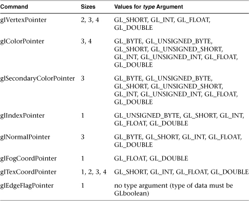
The main difference among the routines is whether size and type are unique or must be specified. For example, a surface normal always has three components, so it is redundant to specify its size. An edge flag is always a single Boolean, so neither size nor type needs to be mentioned. Table 2-4 displays legal values for size and data types.
For OpenGL implementations that support multitexturing, specifying a texture coordinate array with glTexCoordPointer() only affects the currently active texture unit. See “Multitexturing” on page 467 for more information.
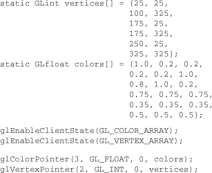
Example 2-9 uses vertex arrays for both RGBA colors and vertex coordinates. RGB floating-point values and their corresponding (x, y) integer coordinates are loaded into the GL_COLOR_ARRAY and GL_VERTEX_ARRAY.
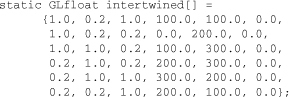
The stride parameter for the gl*Pointer() routines tells OpenGL how to access the data you provide in your pointer arrays. Its value should be the number of bytes between the starts of two successive pointer elements, or zero, which is a special case. For example, suppose you stored both your vertex’s RGB and (x, y, z) coordinates in a single array, such as the following:
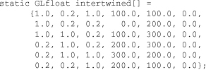
To reference only the color values in the intertwined array, the following call starts from the beginning of the array (which could also be passed as &intertwined[0]) and jumps ahead 6 * sizeof(GLfloat) bytes, which is the size of both the color and vertex coordinate values. This jump is enough to get to the beginning of the data for the next vertex:
glColorPointer(3, GL_FLOAT, 6*sizeof(GLfloat), &intertwined[0]);
For the vertex coordinate pointer, you need to start from further in the array, at the fourth element of intertwined (remember that C programmers start counting at zero):
glVertexPointer(3, GL_FLOAT, 6*sizeof(GLfloat), &intertwined[3]);
If your data is stored similar to the intertwined array above, you may find the approach described in “Interleaved Arrays” on page 88 more convenient for storing your data.
With a stride of zero, each type of vertex array (RGB color, color index, vertex coordinate, and so on) must be tightly packed. The data in the array must be homogeneous; that is, the data must be all RGB color values, all vertex coordinates, or all some other data similar in some fashion.
Until the contents of the vertex arrays are dereferenced, the arrays remain on the client side, and their contents are easily changed. In Step 3, contents of the arrays are obtained, sent to the server, and then sent down the graphics processing pipeline for rendering.
You can obtain data from a single array element (indexed location), from an ordered list of array elements (which may be limited to a subset of the entire vertex array data), or from a sequence of array elements.
|
Compatibility Extension |
|
glArrayElement |
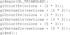
glArrayElement() is usually called between glBegin() and glEnd(). (If called outside, glArrayElement() sets the current state for all enabled arrays, except for vertex, which has no current state.) In Example 2-10, a triangle is drawn using the third, fourth, and sixth vertices from enabled vertex arrays. (Again, remember that C programmers begin counting array locations with zero.)
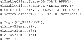
When executed, the latter five lines of code have the same effect as
Since glArrayElement() is only a single function call per vertex, it may reduce the number of function calls, which increases overall performance.
Be warned that if the contents of the array are changed between glBegin() and glEnd(), there is no guarantee that you will receive original data or changed data for your requested element. To be safe, don’t change the contents of any array element that might be accessed until the primitive is completed.
glArrayElement() is good for randomly “hopping around” your data arrays. Similar routines, glDrawElements(), glMultiDrawElements(), and glDrawRangeElements(), are good for hopping around your data arrays in a more orderly manner.
The effect of glDrawElements() is almost the same as this command sequence:
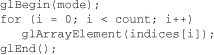
glDrawElements() additionally checks to make sure mode, count, and type are valid. Also, unlike the preceding sequence, executing glDrawElements() leaves several states indeterminate. After execution of glDrawElements(), current RGB color, secondary color, color index, normal coordinates, fog coordinates, texture coordinates, and edge flag are indeterminate if the corresponding array has been enabled.
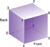
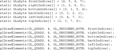
With glDrawElements(), the vertices for each face of the cube can be placed in an array of indices. Example 2-11 shows two ways to use glDrawElements() to render the cube. Figure 2-15 shows the numbering of the vertices used in Example 2-11.
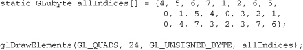
With several primitive types (such as GL_QUADS, GL_TRIANGLES, and GL_LINES), you may be able to compact several lists of indices together into a single array. Since the GL_QUADS primitive interprets each group of four vertices as a single polygon, you may compact all the indices used in Example 2-11 into a single array, as shown in Example 2-12:
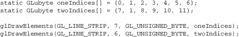
For other primitive types, compacting indices from several arrays into a single array renders a different result. In Example 2-13, two calls to glDrawElements() with the primitive GL_LINE_STRIP render two line strips. You cannot simply combine these two arrays and use a single call to glDrawElements() without concatenating the lines into a single strip that would connect vertices #6 and #7. (Note that vertex #1 is being used in both line strips just to show that this is legal.)
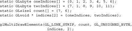
The routine glMultiDrawElements() was introduced in OpenGL Version 1.4 to enable combining the effects of several glDrawElements() calls into a single call.
The effect of glMultiDrawElements() is the same as
The calls to glDrawElements() in Example 2-13 can be combined into a single call of glMultiDrawElements(), as shown in Example 2-14:
Like glDrawElements() or glMultiDrawElements(), glDrawRangeElements() is also good for hopping around data arrays and rendering their contents. glDrawRangeElements() also introduces the added restriction of a range of legal values for its indices, which may increase program performance. For optimal performance, some OpenGL implementations may be able to prefetch (obtain prior to rendering) a limited amount of vertex array data. glDrawRangeElements() allows you to specify the range of vertices to be prefetched.
It is a mistake for vertices in the array indices to reference outside the range [start, end]. However, OpenGL implementations are not required to find or report this mistake. Therefore, illegal index values may or may not generate an OpenGL error condition, and it is entirely up to the implementation to decide what to do.
You can use glGetIntegerv() with GL_MAX_ELEMENTS_VERTICES and GL_MAX_ELEMENTS_INDICES to find out, respectively, the recommended maximum number of vertices to be prefetched and the maximum number of indices (indicating the number of vertices to be rendered) to be referenced. If end – start + 1 is greater than the recommended maximum of prefetched vertices, or if count is greater than the recommended maximum of indices, glDrawRangeElements() should still render correctly, but performance may be reduced.
Not all vertices in the range [start, end] have to be referenced. However, on some implementations, if you specify a sparsely used range, you may unnecessarily process many vertices that go unused.
With glArrayElement(), glDrawElements(), glMultiDrawElements(), and glDrawRangeElements(), it is possible that your OpenGL implementation caches recently processed (meaning transformed, lit) vertices, allowing your application to “reuse” them by not sending them down the transformation pipeline additional times. Take the aforementioned cube, for example, which has six faces (polygons) but only eight vertices. Each vertex is used by exactly three faces. Without gl*Elements(), rendering all six faces would require processing 24 vertices, even though 16 vertices are redundant. Your implementation of OpenGL may be able to minimize redundancy and process as few as eight vertices. (Reuse of vertices may be limited to all vertices within a single glDrawElements() or glDrawRangeElements() call, a single index array for glMultiDrawElements(), or, for glArrayElement(), within one glBegin()/glEnd() pair.)
While glArrayElement(), glDrawElements(), and glDrawRangeElements() “hop around” your data arrays, glDrawArrays() plows straight through them.
The effect of glDrawArrays() is almost the same as this command sequence:
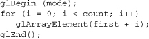
As is the case with glDrawElements(), glDrawArrays() also performs error checking on its parameter values and leaves the current RGB color, secondary color, color index, normal coordinates, fog coordinates, texture coordinates, and edge flag with indeterminate values if the corresponding array has been enabled.
Change the icosahedron drawing routine in Example 2-19 on page 115 to use vertex arrays.
Similar to glMultiDrawElements(), the routine glMultiDrawArrays() was introduced in OpenGL Version 1.4 to combine several glDrawArrays() calls into a single call.
The effect of glMultiDrawArrays() is the same as

As you start working with larger sets of vertex data, you are likely to find that you need to make numerous calls to the OpenGL drawing routines, usually rendering the same type of primitive (such as GL_TRIANGLE_STRIP, for example) that you used in the previous drawing call. Of course, you can use the glMultiDraw*() routines, but they require the overhead of maintaining the arrays for the starting index and length of each primitive.
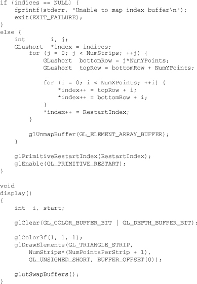
OpenGL Version 3.1 added the ability to restart primitives within the same drawing call by specifying a special value, the primitive restart index, which is specially processed by OpenGL. When the primitive restart index is encountered in a draw call, a new rendering primitive of the same type is started with the vertex following the index. The primitive restart index is specified by the glPrimitiveRestartIndex() routine.
Primitive restarting is controlled by calling glEnable() or glDisable() and specifying GL_PRIMITIVE_RESTART, as demonstrated in Example 2-15.

Advanced
OpenGL Version 3.1 (specifically, GLSL version 1.40) added support for instanced drawing, which provides an additional value—gl_InstanceID, called the instance ID, and accessible only in a vertex shader—that is monotonically incremented for each group of primitives specified.
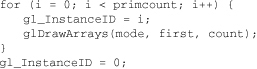
glDrawArraysInstanced() operates similarly to glMultiDrawArrays(), except that the starting index and vertex count (as specified by first and count, respectively) are the same for each call to glDrawArrays().
glDrawArraysInstanced() has the same effect as this call sequence (except that your application cannot manually update gl_InstanceID):
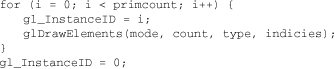
Likewise, glDrawElementsInstanced() performs the same operation, but allows random-access to the data in the vertex array:
The implementation of glDrawElementsInstanced() is shown here:
Advanced
Earlier in this chapter (see “Stride” on page 76), the special case of interleaved arrays was examined. In that section, the array intertwined, which interleaves RGB color and 3D vertex coordinates, was accessed by calls to glColorPointer() and glVertexPointer(). Careful use of stride helped properly specify the arrays:
There is also a behemoth routine, glInterleavedArrays(), that can specify several vertex arrays at once. glInterleavedArrays() also enables and disables the appropriate arrays (so it combines “Step 1: Enabling Arrays” on page 72 and “Step 2: Specifying Data for the Arrays” on page 73). The array intertwined exactly fits one of the 14 data-interleaving configurations supported by glInterleavedArrays(). Therefore, to specify the contents of the array intertwined into the RGB color and vertex arrays and enable both arrays, call
glInterleavedArrays(GL_C3F_V3F, 0, intertwined);
This call to glInterleavedArrays() enables GL_COLOR_ARRAY and GL_VERTEX_ARRAY. It disables GL_SECONDARY_COLOR_ARRAY, GL_INDEX_ARRAY, GL_NORMAL_ARRAY, GL_FOG_COORD_ARRAY, GL_TEXTURE_COORD_ARRAY, and GL_EDGE_FLAG_ARRAY.
This call also has the same effect as calling glColorPointer() and glVertexPointer() to specify the values for six vertices in each array. Now you are ready for Step 3: calling glArrayElement(), glDrawElements(), glDrawRangeElements(), or glDrawArrays() to dereference array elements.
Note that glInterleavedArrays() does not support edge flags.
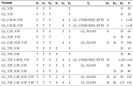
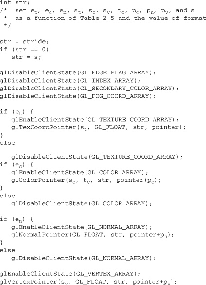
The mechanics of glInterleavedArrays() are intricate and require reference to Example 2-16 and Table 2-5. In that example and table, you’ll see et, ec, and en, which are the Boolean values for the enabled or disabled texture coordinate, color, and normal arrays; and you’ll see st, sc, and sv, which are the sizes (numbers of components) for the texture coordinate, color, and vertex arrays. tc is the data type for RGBA color, which is the only array that can have nonfloating-point interleaved values. pc, pn, and pv are the calculated strides for jumping into individual color, normal, and vertex values; and s is the stride (if one is not specified by the user) to jump from one array element to the next.
|
Compatibility Extension |
|
glInterleavedArrays |
The effect of glInterleavedArrays() is the same as calling the command sequence in Example 2-16 with many values defined in Table 2-5. All pointer arithmetic is performed in units of sizeof(GLubyte).
In Table 2-5, T and F are True and False. f is sizeof(GLfloat). c is 4 times sizeof(GLubyte), rounded up to the nearest multiple of f.
Start by learning the simpler formats, GL_V2F, GL_V3F, and GL_C3F_V3F. If you use any of the formats with C4UB, you may have to use a struct data type or do some delicate type casting and pointer math to pack four unsigned bytes into a single 32-bit word.
For some OpenGL implementations, use of interleaved arrays may increase application performance. With an interleaved array, the exact layout of your data is known. You know your data is tightly packed and may be accessed in one chunk. If interleaved arrays are not used, the stride and size information has to be examined to detect whether data is tightly packed.
Note
glInterleavedArrays() only enables and disables vertex arrays and specifies values for the vertex-array data. It does not render anything. You must still complete “Step 3: Dereferencing and Rendering” on page 77 and call glArrayElement(), glDrawElements(), glDrawRangeElements(), or glDrawArrays() to dereference the pointers and render graphics.
Advanced
There are many operations in OpenGL where you send a large block of data to OpenGL, such as passing vertex array data for processing. Transferring that data may be as simple as copying from your system’s memory down to your graphics card. However, because OpenGL was designed as a client-server model, any time that OpenGL needs data, it will have to be transferred from the client’s memory. If that data doesn’t change, or if the client and server reside on different computers (distributed rendering), that data transfer may be slow, or redundant.
Buffer objects were added to OpenGL Version 1.5 to allow an application to explicitly specify which data it would like to be stored in the graphics server.
Many different types of buffer objects are used in the current versions of OpenGL:
• Vertex data in arrays can be stored in server-side buffer objects starting with OpenGL Version 1.5. They are described in “Using Buffer Objects with Vertex-Array Data” on page 102 of this chapter.
• Support for storing pixel data, such as texture maps or blocks of pixels, in buffer objects was added into OpenGL Version 2.1 It is described in “Using Buffer Objects with Pixel Rectangle Data” in Chapter 8.
• Version 3.1 added uniform buffer objects for storing blocks of uniform-variable data for use with shaders.
You will find many other features in OpenGL that use the term “objects,” but not all apply to storing blocks of data. For example, texture objects (introduced in OpenGL Version 1.1) merely encapsulate various state settings associated with texture maps (See “Texture Objects” on page 437). Likewise, vertex-array objects, added in Version 3.0, encapsulate the state parameters associated with using vertex arrays. These types of objects allow you to alter numerous state settings with many fewer function calls. For maximum performance, you should try to use them whenever possible, once you’re comfortable with their operation.
In OpenGL Version 3.0, any nonzero unsigned integer may used as a buffer object identifier. You may either arbitrarily select representative values or let OpenGL allocate and manage those identifiers for you. Why the difference? By having OpenGL allocate identifiers, you are guaranteed to avoid an already used buffer object identifier. This helps to eliminate the risk of modifying data unintentionally. In fact, OpenGL Version 3.1 requires that all object identifiers be generated, disallowing user-defined names.
To have OpenGL allocate buffer objects identifiers, call glGenBuffers().
You can also determine whether an identifier is a currently used buffer object identifier by calling glIsBuffer().
To make a buffer object active, it needs to be bound. Binding selects which buffer object future operations will affect, either for initializing data or using that buffer for rendering. That is, if you have more than one buffer object in your application, you’ll likely call glBindBuffer() multiple times: once to initialize the object and its data, and then subsequent times either to select that object for use in rendering or to update its data.
To disable use of buffer objects, call glBindBuffer() with zero as the buffer identifier. This switches OpenGL to the default mode of not using buffer objects.
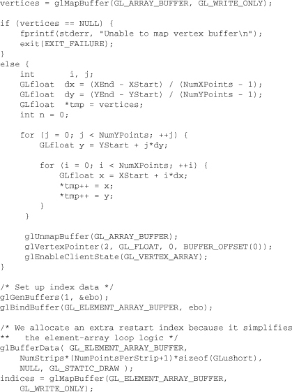
Once you’ve bound a buffer object, you need to reserve space for storing your data. This is done by calling glBufferData().
glBufferData() first allocates memory in the OpenGL server for storing your data. If you request too much memory, a GL_OUT_OF_MEMORY error will be set. Once the storage has been reserved, and if the data parameter is not NULL, size units of storage (usually bytes) are copied from the client’s memory into the buffer object. However, if you need to dynamically load the data at some point after the buffer is created, pass NULL in for the data pointer. This will reserve the appropriate storage for your data, but leave it uninitialized.
The final parameter to glBufferData(), usage, is a performance hint to OpenGL. Based upon the value you specify for usage, OpenGL may be able to optimize the data for better performance, or it can choose to ignore the hint. There are three operations that can be done to buffer object data:
- Drawing—the client specifies data that is used for rendering.
- Reading—data values are read from an OpenGL buffer (such as the framebuffer) and used in the application in various computations not immediately related to rendering.
- Copying—data values are read from an OpenGL buffer and then used as data for rendering.
Additionally, depending upon how often you intend to update the data, there are various operational hints for describing how often the data will be read or used in rendering:
• Stream mode—you specify the data once, and use it only a few times in drawing or other operations.
• Static mode—you specify the data once, but use the values often.
• Dynamic mode—you may update the data often and use the data values in the buffer object many times as well.
Possible values for usage are described in Table 2-6.

There are two methods for updating data stored in a buffer object. The first method assumes that you have data of the same type prepared in a buffer in your application. glBufferSubData() will replace some subset of the data in the bound buffer object with the data you provide.
The second method allows you more control over which data values are updated in the buffer. glMapBuffer() and glMapBufferRange() return a pointer to the buffer object memory, into which you can write new values (or simply read the data, depending on your choice of memory access permissions), just as if you were assigning values to an array. When you’ve completed updating the values in the buffer, you call glUnmapBuffer() to signify that you’ve completed updating the data.
glMapBuffer() provides access to the entire set of data contained in the buffer object. This approach is useful if you need to modify much of the data in buffer, but may be inefficient if you have a large buffer and need to update only a small portion of the values.
When you’ve completed accessing the storage, you can unmap the buffer by calling glUnmapBuffer().
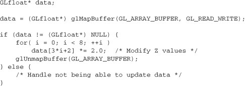
As a simple example of how you might selectively update elements of your data, we’ll use glMapBuffer() to obtain a pointer to the data in a buffer object containing three-dimensional positional coordinates, and then update only the z-coordinates.
If you need to update only a relatively small number of values in the buffer (as compared to its total size), or small contiguous ranges of values in a very large buffer object, it may be more efficient to use glMapBufferRange(). It allows you to map only the range of data values you need.
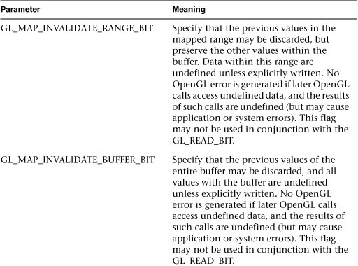
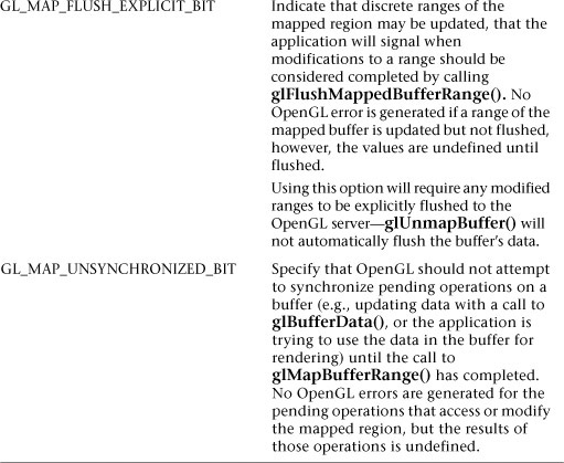
Using glMapBufferRange(), you can specify optional hints by setting additional bits within access. These flags describe how the OpenGL server needs to preserve data that was originally in the buffer before you mapped it. The hints are meant to aid the OpenGL implementation in determining which data values it needs to retain, or for how long, to keep any internal copies of the data correct and consistent.
As described in Table 2-7, specifying GL_MAP_FLUSH_EXPLICIT_BIT in the access flags when mapping a buffer region with glMapBufferRange() requires ranges modified within the mapped buffer to be indicated to the OpenGL by a call to glFlushMappedBufferRange().
On some occasions, you may need to copy data from one buffer object to another. In versions of OpenGL prior to Version 3.1, this would be a two-step process:
- Copy the data from the buffer object into memory in your application. You would do this either by mapping the buffer and copying it into a local memory buffer, or by calling glGetBufferSubData() to copy the data from the server.
- Update the data in another buffer object by binding to the new object and then sending the new data using glBufferData() (or glBufferSubData() if you’re replacing only a subset). Alternatively, you could map the buffer, and then copy the data from a local memory buffer into the mapped buffer.
In OpenGL Version 3.1, the glCopyBufferSubData() command copies data without forcing it to make a temporary stop in your application’s memory.
When you’re finished with a buffer object, you can release its resources and make its identifier available by calling glDeleteBuffers(). Any bindings to currently bound objects that are deleted are reset to zero.
To store your vertex-array data in buffer objects, you will need to add a few steps to your application.
- (Optional) Generate buffer object identifiers.
- Bind a buffer object, specifying that it will be used for either storing vertex data or indices.
- Request storage for your data, and optionally initialize those data elements.
- Specify offsets relative to the start of the buffer object to initialize the vertex-array functions, such as glVertexPointer().
- Bind the appropriate buffer object to be utilized in rendering.
- Render using an appropriate vertex-array rendering function, such as glDrawArrays() or glDrawElements().
If you need to initialize multiple buffer objects, you will repeat steps 2 through 4 for each buffer object.
Both “formats” of vertex-array data are available for use in buffer objects. As described in “Step 2: Specifying Data for the Arrays,” vertex, color, lighting normal, or any other type of associated vertex data can be stored in a buffer object. Additionally, interleaved vertex array data, as described in “Interleaved Arrays,” can also be stored in a buffer object. In either case, you would create a single buffer object to hold all of the data to be used as vertex arrays.
As compared to specifying a memory address in the client’s memory where OpenGL should access the vertex-array data, you specify the offset in machine units (usually bytes) to the data in the buffer. To help illustrate computing the offset, and to frustrate the purists in the audience, we’ll use the following macro to simplify expressing the offset:
#define BUFFER_OFFSET(bytes) ((GLubyte*) NULL + (bytes))
For example, if you had floating-point color and position data for each vertex, perhaps represented as the following array
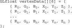
that were used to initialize the buffer object, you could specify the data as two separate vertex array calls, one for colors and one for vertices:
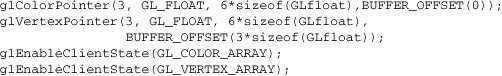
Conversely, since the data in vertexData matches a format for an interleaved vertex array, you could use glInterleavedArrays() for specifying the vertex-array data:
glInterleavedArrays(GL_C3F_V3F, 0, BUFFER_OFFSET(0));
Putting this all together, Example 2-17 demonstrates how buffer objects of vertex data might be used. The example creates two buffer objects, one containing vertex data and the other containing index data.
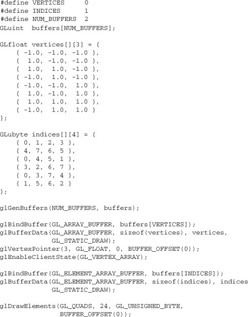
As your programs grow larger and use more models, you will probably find that you switch between multiple sets of vertex arrays each frame. Depending on how many vertex attributes you’re using for each vertex, the number of calls—such as to glVertexPointer()—may start to become large. Vertex-array objects bundle collections of calls for setting the vertex array’s state. After being initialized, you can quickly change between different sets of vertex arrays with a single call.
To create a vertex-array object, first call glGenVertexArrays(), which will create the requested number of uninitialized objects:
After creating your vertex-array objects, you’ll need to initialize the new objects, and associate the set of vertex-array data that you want to enable with the individual allocated objects. You do this with the glBindVertexArray() routine. Once you initialize all of your vertex-array objects, you can use glBindVertexArray() to switch between the different sets of vertex arrays that you’ve set up.
Example 2-18 demonstrates switching between two sets of vertex arrays using vertex-arrays objects.

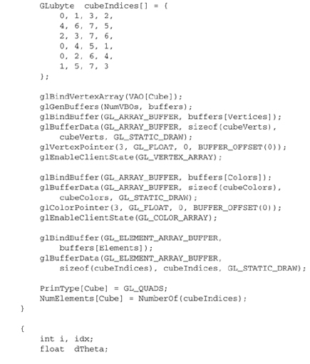
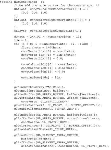
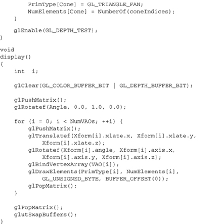
To delete vertex-array objects and release their names for reuse, call glDeleteVertexArrays(). If you’re using buffer objects for storing data, they are not deleted when the vertex-array object referencing them is deleted. They continue to exist (until you delete them). The only change that occurs is if the buffer objects were currently bound when you deleted the vertex-array object, they become unbound.
Finally, if you need to determine whether a particular value might represent an allocated (but not necessarily initialized) vertex-array object, you can check by calling glIsVertexArray().
In “Basic State Management” you saw how to set or query an individual state or state variable. You can also save and restore the values of a collection of related state variables with a single command.
OpenGL groups related state variables into an attribute group. For example, the GL_LINE_BIT attribute consists of five state variables: the line width, the GL_LINE_STIPPLE enable status, the line stipple pattern, the line stipple repeat counter, and the GL_LINE_SMOOTH enable status. (See “Antialiasing” in Chapter 6.) With the commands glPushAttrib() and glPopAttrib(), you can save and restore all five state variables at once.
Some state variables are in more than one attribute group. For example, the state variable GL_CULL_FACE is part of both the polygon and the enable attribute groups.
In OpenGL Version 1.1, there are now two different attribute stacks. In addition to the original attribute stack (which saves the values of server state variables), there is also a client attribute stack, accessible by the commands glPushClientAttrib() and glPopClientAttrib().
In general, it’s faster to use these commands than to get, save, and restore the values yourself. Some values might be maintained in the hardware, and getting them might be expensive. Also, if you’re operating on a remote client, all the attribute data has to be transferred across the network connection and back as it is obtained, saved, and restored. However, your OpenGL implementation keeps the attribute stack on the server, avoiding unnecessary network delays.
There are about 20 different attribute groups, which can be saved and restored by glPushAttrib() and glPopAttrib(). There are two client attribute groups, which can be saved and restored by glPushClientAttrib() and glPopClientAttrib(). For both server and client, the attributes are stored on a stack, which has a depth of at least 16 saved attribute groups. (The actual stack depths for your implementation can be obtained using GL_MAX_ATTRIB_STACK_DEPTH and GL_MAX_CLIENT_ATTRIB_STACK_DEPTH with glGetIntegerv().) Pushing a full stack or popping an empty one generates an error.
(See the tables in Appendix B to find out exactly which attributes are saved for particular mask values—that is, which attributes are in a particular attribute group.)
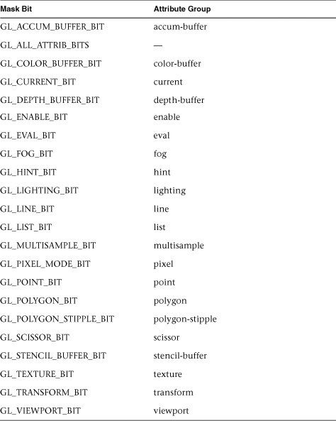
|
Compatibility Extension |
|
glPushAttrib glPopAttrib GL_ACCUM_BUFFER_BIT GL_ALL_ATTRIB_BITS GL_COLOR_BUFFER_BIT GL_CURRENT_BIT GL_DEPTH_BUFFER_BIT GL_ENABLE_BIT GL_EVAL_BIT GL_FOG_BIT GL_HINT_BIT GL_LIGHTING_BIT GL_LINE_BIT GL_LIST_BIT GL_MULTISAMPLE_BIT GL_PIXEL_MODE_BIT GL_POINT_BIT GL_POLYGON_BIT GL_POLYGON_STIPPLE_BIT GL_SCISSOR_BIT GL_STENCIL_BUFFER_BIT GL_TEXTURE_BIT GL_TRANSFORM_BIT GL_VIEWPORT_BIT |
The special mask GL_ALL_ATTRIB_BITS is used to save and restore all the state variables in all the attribute groups.
Two client attribute groups, feedback and select, cannot be saved or restored with the stack mechanism.
Table 2-9. Client Attribute Groups
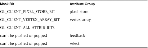
|
Compatibility Extension |
|
glPushClientAttrib glPopClientAttrib GL_CLIENT_PIXEL_STORE_BIT GL_CLIENT_VERTEX_ARRAY_BIT GL_CLIENT_ALL_ATTRIB_BITS |
Following are some techniques that you can use as you build polygonal approximations of surfaces. You might want to review this section after you’ve read Chapter 5 on lighting and Chapter 7 on display lists. The lighting conditions affect how models look once they’re drawn, and some of the following techniques are much more efficient when used in conjunction with display lists. As you read these techniques, keep in mind that when lighting calculations are enabled, normal vectors must be specified to get proper results.
Constructing polygonal approximations to surfaces is an art, and there is no substitute for experience. This section, however, lists a few pointers that might make it a bit easier to get started.
• Keep polygon orientations (windings) consistent. Make sure that when viewed from the outside, all the polygons on the surface are oriented in the same direction (all clockwise or all counterclockwise). Consistent orientation is important for polygon culling and two-sided lighting. Try to get this right the first time, as it’s excruciatingly painful to fix the problem later. (If you use glScale*() to reflect geometry around some axis of symmetry, you might change the orientation with glFrontFace() to keep the orientations consistent.)
• When you subdivide a surface, watch out for any nontriangular polygons. The three vertices of a triangle are guaranteed to lie on a plane; any polygon with four or more vertices might not. Nonplanar polygons can be viewed from some orientation such that the edges cross each other, and OpenGL might not render such polygons correctly.
• There’s always a trade-off between the display speed and the quality of the image. If you subdivide a surface into a small number of polygons, it renders quickly but might have a jagged appearance; if you subdivide it into millions of tiny polygons, it probably looks good but might take a long time to render. Ideally, you can provide a parameter to the subdivision routines that indicates how fine a subdivision you want, and if the object is farther from the eye, you can use a coarser subdivision. Also, when you subdivide, use large polygons where the surface is relatively flat, and small polygons in regions of high curvature.
• For high-quality images, it’s a good idea to subdivide more on the silhouette edges than in the interior. If the surface is to be rotated relative to the eye, this is tougher to do, as the silhouette edges keep moving. Silhouette edges occur where the normal vectors are perpendicular to the vector from the surface to the viewpoint—that is, when their vector dot product is zero. Your subdivision algorithm might choose to subdivide more if this dot product is near zero.
• Try to avoid T-intersections in your models (see Figure 2-16). As shown, there’s no guarantee that the line segments AB and BC lie on exactly the same pixels as the segment AC. Sometimes they do, and sometimes they don’t, depending on the transformations and orientation. This can cause cracks to appear intermittently in the surface.

• If you’re constructing a closed surface, be sure to use exactly the same numbers for coordinates at the beginning and end of a closed loop, or you can get gaps and cracks due to numerical round-off. Here’s an example of bad code for a two-dimensional circle:
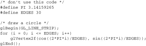
The edges meet exactly only if your machine manages to calculate exactly the same values for the sine and cosine of 0 and of (2*PI*EDGES/EDGES). If you trust the floating-point unit on your machine to do this right, the authors have a bridge they’d like to sell you... To correct the code, make sure that when i == EDGES, you use 0 for the sine and cosine, not 2*PI*EDGES/EDGES. (Or simpler still, use GL_LINE_LOOP instead of GL_LINE_STRIP, and change the loop termination condition to i < EDGES.)
To illustrate some of the considerations that arise in approximating a surface, let’s look at some example code sequences. This code concerns the vertices of a regular icosahedron (which is a Platonic solid composed of 20 faces that span 12 vertices, the face of each being an equilateral triangle). An icosahedron can be considered a rough approximation of a sphere. Example 2-19 defines the vertices and triangles making up an icosahedron and then draws the icosahedron.
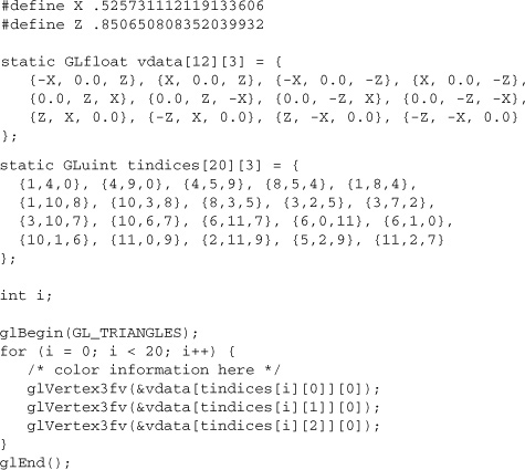
The strange numbers X and Z are chosen so that the distance from the origin to any of the vertices of the icosahedron is 1.0. The coordinates of the 12 vertices are given in the array vdata[][], where the zeroth vertex is {−X, 0.0, Z}, the first is {X, 0.0, Z}, and so on. The array tindices[][] tells how to link the vertices to make triangles. For example, the first triangle is made from the zeroth, fourth, and first vertices. If you take the vertices for triangles in the order given, all the triangles have the same orientation.
The line that mentions color information should be replaced by a command that sets the color of the ith face. If no code appears here, all faces are drawn in the same color, and it will be impossible to discern the three-dimensional quality of the object. An alternative to explicitly specifying colors is to define surface normals and use lighting, as described in the next subsection.
Note
In all the examples described in this section, unless the surface is to be drawn only once, you should probably save the calculated vertex and normal coordinates so that the calculations don’t need to be repeated each time the surface is drawn. This can be done using your own data structures or by constructing display lists (see Chapter 7).
If a surface is to be lit, you need to supply the vector normal to the surface. Calculating the normalized cross product of two vectors on that surface provides their normal vector. With the flat surfaces of an icosahedron, all three vertices defining a surface have the same normal vector. In this case, the normal needs to be specified only once for each set of three vertices. The code in Example 2-20 can replace the “color information here” line in Example 2-19 for drawing the icosahedron.
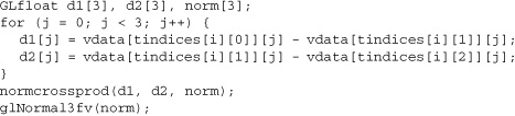
The function normcrossprod() produces the normalized cross product of two vectors, as shown in Example 2-21.
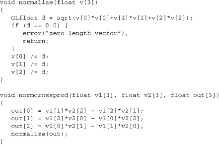
If you’re using an icosahedron as an approximation for a shaded sphere, you’ll want to use normal vectors that are perpendicular to the true surface of the sphere, rather than perpendicular to the faces. For a sphere, the normal vectors are simple; each points in the same direction as the vector from the origin to the corresponding vertex. Since the icosahedron vertex data is for an icosahedron of radius 1, the normal data and vertex data are identical. Here is the code that would draw an icosahedral approximation of a smoothly shaded sphere (assuming that lighting is enabled, as described in Chapter 5):
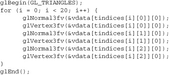
A 20-sided approximation to a sphere doesn’t look good unless the image of the sphere on the screen is quite small, but there’s an easy way to increase the accuracy of the approximation. Imagine the icosahedron inscribed in a sphere, and subdivide the triangles as shown in Figure 2-17. The newly introduced vertices lie slightly inside the sphere, so push them to the surface by normalizing them (dividing them by a factor to make them have length 1). This subdivision process can be repeated for arbitrary accuracy. The three objects shown in Figure 2-17 use 20, 80, and 320 approximating triangles, respectively.

Example 2-22 performs a single subdivision, creating an 80-sided spherical approximation.
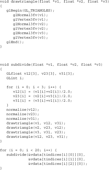
Example 2-23 is a slight modification of Example 2-22 that recursively subdivides the triangles to the proper depth. If the depth value is 0, no subdivisions are performed, and the triangle is drawn as is. If the depth is 1, a single subdivision is performed, and so on.
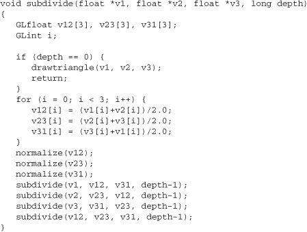
A recursive subdivision technique such as the one described in Example 2-23 can be used for other types of surfaces. Typically, the recursion ends if either a certain depth is reached or some condition on the curvature is satisfied (highly curved parts of surfaces look better with more subdivision).
To look at a more general solution to the problem of subdivision, consider an arbitrary surface parameterized by two variables, u[0] and u[1]. Suppose that two routines are provided:
void surf(GLfloat u[2], GLfloat vertex[3], GLfloat normal[3]);
float curv(GLfloat u[2]);
If u[] is passed to surf(), the corresponding three-dimensional vertex and normal vectors (of length 1) are returned. If u[] is passed to curv(), the curvature of the surface at that point is calculated and returned. (See an introductory textbook on differential geometry for more information about measuring surface curvature.)
Example 2-24 shows the recursive routine that subdivides a triangle until either the maximum depth is reached or the maximum curvature at the three vertices is less than some cutoff.