
Magnetic microrobots for microbiology
Edward B. Steager⁎; Denise Wong⁎; Mahmut Selman Sakar†; Vijay Kumar⁎ ⁎University of Pennsylvania, Philadelphia, PA, United States
†Swiss Federal Institute of Technology in Lausanne, Lausanne, Switzerland
Abstract
Transport of individual cells or chemical payloads on a subcellular scale is an enabling tool for the study of cellular communication, cell migration, and other localized phenomena. We present a magnetically actuated robotic system capable of fully automated manipulation of cells and microbeads. Our strategy uses autofluorescent robotic transporters and fluorescently labeled microbeads to aid tracking and control in optically obstructed environments. We demonstrate automated delivery of microbeads infused with chemicals to specified positions on neurons. This system is compatible with standard upright and inverted light microscopes and is capable of applying forces less than 1 pN for precision positioning tasks. We additionally present a methodology for manipulation of multiple magnetic microrobots using globally applied fields.
Keywords
Microrobot; Micromanipulation; Cell manipulation; Cell sorting; Multirobot
Acknowledgments
We gratefully acknowledge the support of ARO Grant W911NF-05-1-0219, the Penn Genome Frontiers Institute, the Keck Foundation, ONR Grant N00014-07-1-0829, and NSF grant CNS-1446592.
9.1 Introduction
As the length scales of robotic systems continue to decrease, one of the emerging applications is the manipulation of single biological cells in fluid environments [1]. Single-cell manipulation has traditionally been achieved with pipettes, and more recently with optical traps, or microelectromechanical (MEMS) devices [2–5]. As an alternative approach, tetherless, remotely controlled microrobots have the potential to be used as medical tools for the localized delivery of chemicals, cells and other biological substances in vivo and in vitro [6,7]. A variety of techniques have been explored for the wireless actuation of microrobots [8]. Magnetic fields have been the primary method of propulsion, as they are minimally invasive and accepted as harmless in the medical field (i.e. magnetic resonance imaging) and in biological environments [9]. Several untethered magnetic microrobots have been developed and employed for micromanipulation tasks [10–16]. We introduce in this chapter a fully automated microrobotic system for manipulating individual cells and locally delivering chemicals [17], paying particular attention to appropriate scaling of robot size, automation and geometry.
The most appropriate workspace for robotic single cell manipulation is the stage of inverted or upright light microscopes. Such microscopes are ubiquitous in life science research laboratories, and include essential capabilities such as bright field and fluorescence microscopy. Therefore, the integration of the full design includes not only an appropriate robot design, but also a compact controller that is compatible with the stage of existing microscopes. By integrating the design into existing microscopes, imaging capture capabilities of the microscopes may also be harnessed.
One of the most important length scales to consider for the system is the workspace for the robot. When working with single cells, fine details of individual cells must be resolved. The mammalian cell is an entity with typical dimensions of tens of microns. This requires a magnification of at least 40×. The workspace is then 150 μm × 150 μm. Based on this, it becomes clear that the robot must not only be small relative to the workspace and have sizes comparable to those of target cells, but also that precise control of movement is very important. In fact, rapid movements may cause significant disturbances to the microenvironment.
Robotic manipulators on the scale of cells offer significant benefits beyond simply moving cells. Wirelessly controlled (i.e. untethered) cell-sized robots are highly non-invasive. At this length scale, where viscous fluid forces dominate inertial forces, motile microrobots cause very little mixing or agitation of the surrounding environment. This is a significant advantage over suction pipetting for life scientists, since pipettes cause relatively large fluid disturbances. Traditionally, the focus of robotic manipulators has been centered on applying mechanical forces. However, on the scale of individual cells, the understanding of the word manipulation itself must be expanded to include chemical manipulation of local microenvironments. To a great extent, research in single cell life sciences is concerned with biochemistry. Molecular gradients are important for various biological processes such as cell migration, differentiation during embryonic morphogenesis, and disease progression in cancer [18]. The ability to apply a combination of different manipulation cues will bring new opportunities to study single cell behavior, especially for defining conditions that drive cell pathology.
In this chapter, a magnetic microrobot and controller setup is described which satisfies the aforementioned design constraints. The robot, which is only slightly larger than the neuron cell, has been designed to work on a scale appropriate for the working space of a light microscope. Composed of iron oxide nanoparticles embedded in a polymer, the robot is fully biocompatible and is patterned using a single-mask photolithographic process. Furthermore, due to the sub-micron resolution of the photolithographic micromachining process, the robot may be scaled appropriately for geometric compatibility with different cell types. A five coil magnetic controller was designed for rapid integration with existing microscopes. Visual servoing was incorporated for either teleoperation or automated micromanipulation. We also present results on the integration of biodegradable polymeric microbeads designed for targeted drug delivery. We show that these beads are capable of creating localized gradients and can be positioned at target locations in a fully automated fashion.
Additionally, there are many applications in which it would be desirable to operate several microrobots simultaneously. For example, we might wish to parallelize tasks such as cell sorting, or perhaps use multiple robots to perform an operation such as creating complex chemical cues. In the latter portion of this chapter we present analysis, simulation, and experimental evidence to use electromagnetic coils to simultaneously control multiple magnetic robotic manipulators [19].
9.2 Single microrobot methods
9.2.1 Fabrication of microrobots
In previous work, we developed a single step fabrication process for biocompatible magnetic microtransporters that did not require subsequent lithography or etching processes [11]. We fabricated the microstructures on glass slides using a ferromagnetic photoresist. The composite photoresist was prepared by mixing iron oxide powder (spherical, 50 nm in diameter, Alfa Aesar, IL, USA) with SU8-10 photoresist (MicroChem, MA, USA) in a glass Petri dish until it yielded a homogeneous suspension. Although magnetite nanoparticles are opaque, standard lithography still works as reflection, scattering and diffraction of light from the particles assist in the proper exposure of the photoresist [20].
The fabrication sequence is shown in Fig. 9.1. The first spin-coating procedure is used to prepare the non-toxic water-soluble sacrificial dextran layer [21]. We need this layer to release microstructures into the fluidic chamber without causing any structural damage. Next, a thin layer (2 μm) of pure SU8-2 is spin coated. This extra layer ensures better release of microtransporters and helps to obtain a more uniform coating of composite polymer in the following step. Finally, the composite ferromagnetic photoresist is spin coated and the exposed substrate is post-baked and developed in Propylene Glycol Monomethyl Ether Acetate (PGMEA). We optimize our fabrication procedure for a specific weight ratio (5% by weight) and photoresist thickness (10 μm) and fabricate 30 × 30 × 10 μm3 U-shaped microtransporters [22].
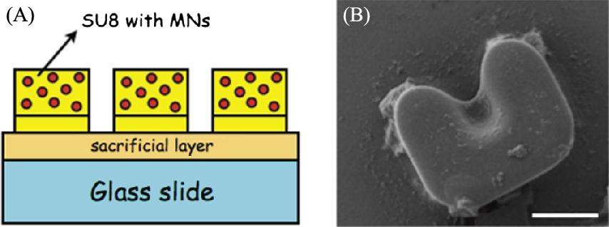
We magnetize our microtransporters using a rectangular neodymium–iron–boron (NdFeB) magnet with a surface field of 6450 Gauss (K&J Magnetics, Jamison, PA) in the direction of the opening of the U shape so that the magnetization vector points towards that direction. They are released on a glass slide by bringing the chip with patterned microstructures into contact with DI water. They can also be trapped under a closed microfluidic channel and released by filling the channel with water [23].
9.2.2 Fabrication of PLGA beads
Poly(lactic-co-glycolic acid) (PLGA) microbeads were composed for the delivery of chemical payloads. The microbeads are biocompatible and degrade slowly, allowing a localized, controlled release of an encapsulated drug, fluorophore, or other chemical. These polymeric beads are composed via a single oil/water emulsion procedure. A 10% (w/v) PLGA/DCM + chemical payload mixture is added under agitation to a 1% aqueous PVA solution, and subsequently stirred for 8 h in an open container (see Fig. 9.2).
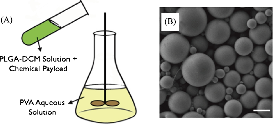
After mixing beads may be separated by centrifugation and removal of supernatant. For long-term storage, the beads may be lyophilized or simply vacuum desiccated.
9.2.3 Experimental setup
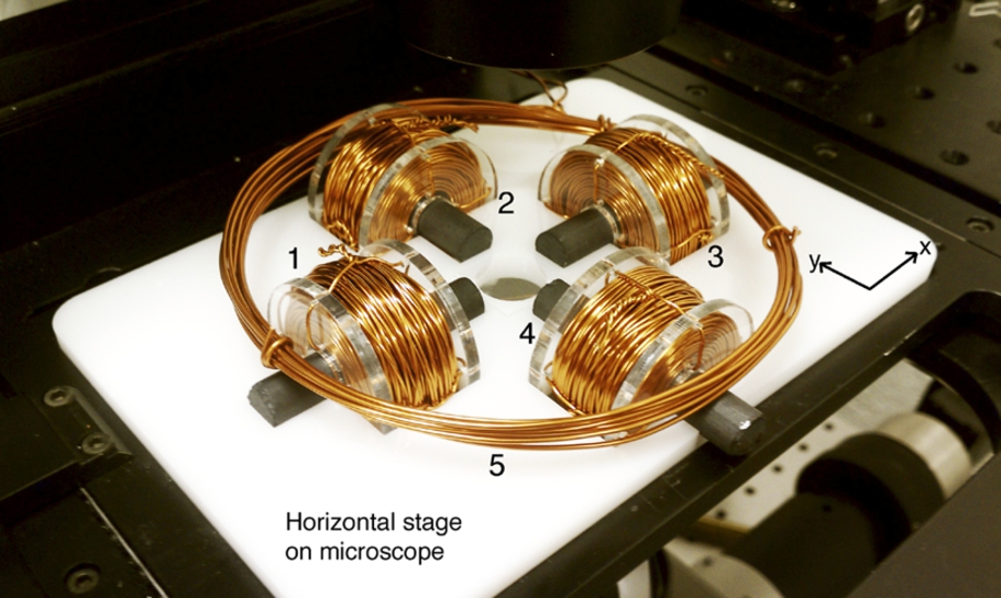
The experimental setup consists of four identical in-plane electromagnetic coils and one out-of-plane electromagnetic coil which is used to induce a stick–slip motion (see Fig. 9.3). Each coil is composed of 22 gauge copper magnetic wire and has 300 turns. Each ferrite core is 50.8 mm long and has a cross-sectional diameter of 9.5 mm. The coils are integrated with an acrylic frame that allows experimentation with both inverted and upright microscopes, and are independently driven with switchable power supplies controlled through a National Instruments PCI-6713 DAQ. Imaging is performed on either a Nikon inverted microscope using bright field or Zeiss upright microscope using fluorescence. Videos are captured using a CCD camera, and video processing is performed using standard Open CV libraries.
9.3 Modeling and control for single magnetic microrobots
9.3.1 Model of magnetic fields
Actuation of robots in this experimental setup relies on applying a magnetic pulling force. The four in-plane coils can be energized individually or in pairs to create motion in any direction in the plane. The robot is pre-magnetized, and its dipole will align with the applied field. The orientation of the robot is dependent upon the direction of current applied to the coils. This is particularly effective for the style of transport used in this work. The cup-like shape is effective at trapping and stabilizing objects while they are being pushed. When the target object has been delivered to its goal position, the current in the coils may be reversed, enabling the robot to maintain orientation while reversing direction. This allows the object (microbead, cell, etc.) to remain in place while the robot moves to the next task.
Ferro-magnetic microrobots are demagnetized when they experience hysteresis, which is the process in which a magnets' magnetization is either gained or lost in a larger field. If the microrobots' magnetization vector M is in the same direction as the applied field B then the microrobot will become magnetized until it reaches a maximum magnetization called the saturation magnetization [8]. Once the external field is removed the microrobot will have a magnetization value equal called its remanent magnetization [24]. However, if a field H equal to the intrinsic coercivity of the ferromagnetic microrobot is applied in the opposite direction of M, the microrobot will lose its magnetization. This is important because if the microrobot is demagnetized during operation it will become unresponsive and ineffective. One way to avoid demagnetization is to minimize the angle between B and M so that torque will be produced on the microrobot instead of demagnetization [8]. Torque produced on a microrobot is given by Eq. (9.1):
Eq. (9.1) illustrates how the microrobot seeks to align itself with the B field. When the microrobot is close to the center axis of the dipole moment field source, the force lines that pull the microrobot closer to the source may be modeled as being the same as those of B; however, when the microrobot is considerably farther away from the center axis, the force and flux lines no longer coincide. Near the axis of the dipole moment, the force F may simply be modeled with Eq. (9.2), where V is the volume of the magnetized object, B is the field from the dipole moment coil and M is the magnetization of the microrobot:
In our experimental setup, the workspace is relatively small compared to the size of the electromagnets, and can be reasonably approximated as lying along the center axes of the electromagnets. It should be noted that de-magnetization is also limited since the dipole of the robot is aligned with the magnetic field, which limits the effects of hysteresis.
9.3.2 Control
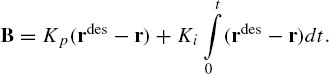
Since the inertial forces at smaller scales are negligible compared to actuator forces and drag forces due to friction and drag, the robot can be modeled as a first order system. Further, we can independently control the components of magnetic field B allowing independent control of the forces in the two horizontal directions [25]. Thus we can model the system as two decoupled, first order differential equations. To follow a specified trajectory, ![]() , we apply a proportional plus integral controller to drive the magnetic field
, we apply a proportional plus integral controller to drive the magnetic field
9.3.3 Planning
The trajectory is derived from a simple search-based planning algorithm. We discretize the environment into a rectangular grid and use an 8-connected grid to generate a graph representation for the environment (Fig. 9.13). We use the ![]() algorithm to derive two trajectories: the path from the robot initial position to the selected bead; and the path from the bead to the selected neuron. Since the robot entraps the bead in an open cup-like shape, it is necessary to consider the direction of approach. Once the robot is in contact with the bead, it is important that its motion remains in a consistent direction so the bead does not slip away from the robot on the path to the target location. Therefore, the algorithm ensures that the robot approaches and pushes from the correct direction to ensure a relatively simple, straight path from bead to cell. Once the path is determined, Eq. (9.3) is used to drive the robot.
algorithm to derive two trajectories: the path from the robot initial position to the selected bead; and the path from the bead to the selected neuron. Since the robot entraps the bead in an open cup-like shape, it is necessary to consider the direction of approach. Once the robot is in contact with the bead, it is important that its motion remains in a consistent direction so the bead does not slip away from the robot on the path to the target location. Therefore, the algorithm ensures that the robot approaches and pushes from the correct direction to ensure a relatively simple, straight path from bead to cell. Once the path is determined, Eq. (9.3) is used to drive the robot.
9.4 Vision-based tracking
Automated visual servoing of magnetic microrobots can be accomplished either via bright field or fluorescence microscopy. Bright field microscopy typically reveals all objects with dimensions larger than the wavelength of visible light. However, for heavily occluded images, such as images of plated neurons, fluorescence microscopy offers significant benefits in terms of optical filtering. In fluorescence microscopy, the only elements which appear are those which have been fluorescently tagged, which simplifies real-time processing and feedback.
9.4.1 Tracking with bright field microscopy
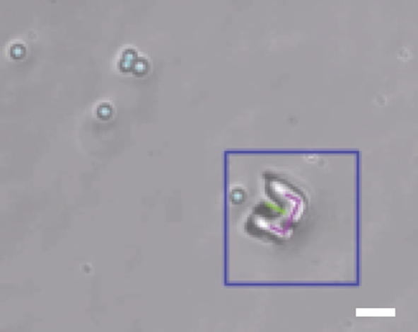
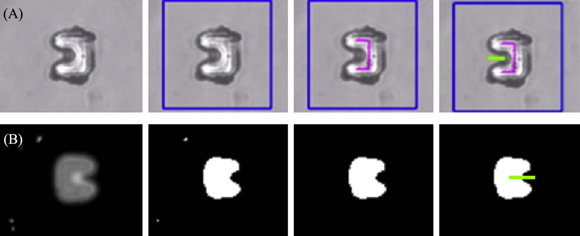
The appearance of microtransporters under bright field illumination varies based on focal plane, contact with microbeads or cells, and the attachment of debris to the surface. For these reasons and in order to alleviate the burden on experimental procedure, very few constraints are placed on expected image backgrounds or absolute image characteristics. Instead, relative measures are preferred wherever possible, while each processing stage refines the region of interest fed into subsequent stages. The output of the entire tracking scheme running at 30 Hz is highlighted in Fig. 9.4.
9.4.2 Tracking with fluorescence microscopy
In the biological sciences, fluorescence microscopy is a technique often used to reveal cellular structure or sub cellular processes. Fluorophores are designed to generally label particular types of cells and organelles, or even to indicate the presence of particular molecules. In contrast to bright field microscopy, it has the significant advantage of revealing only the targeted structure. This technique, which is already integrated with many microscopes, can be used to simplify the tracking and targeting of robotic microtransporters, microbeads, and targets.
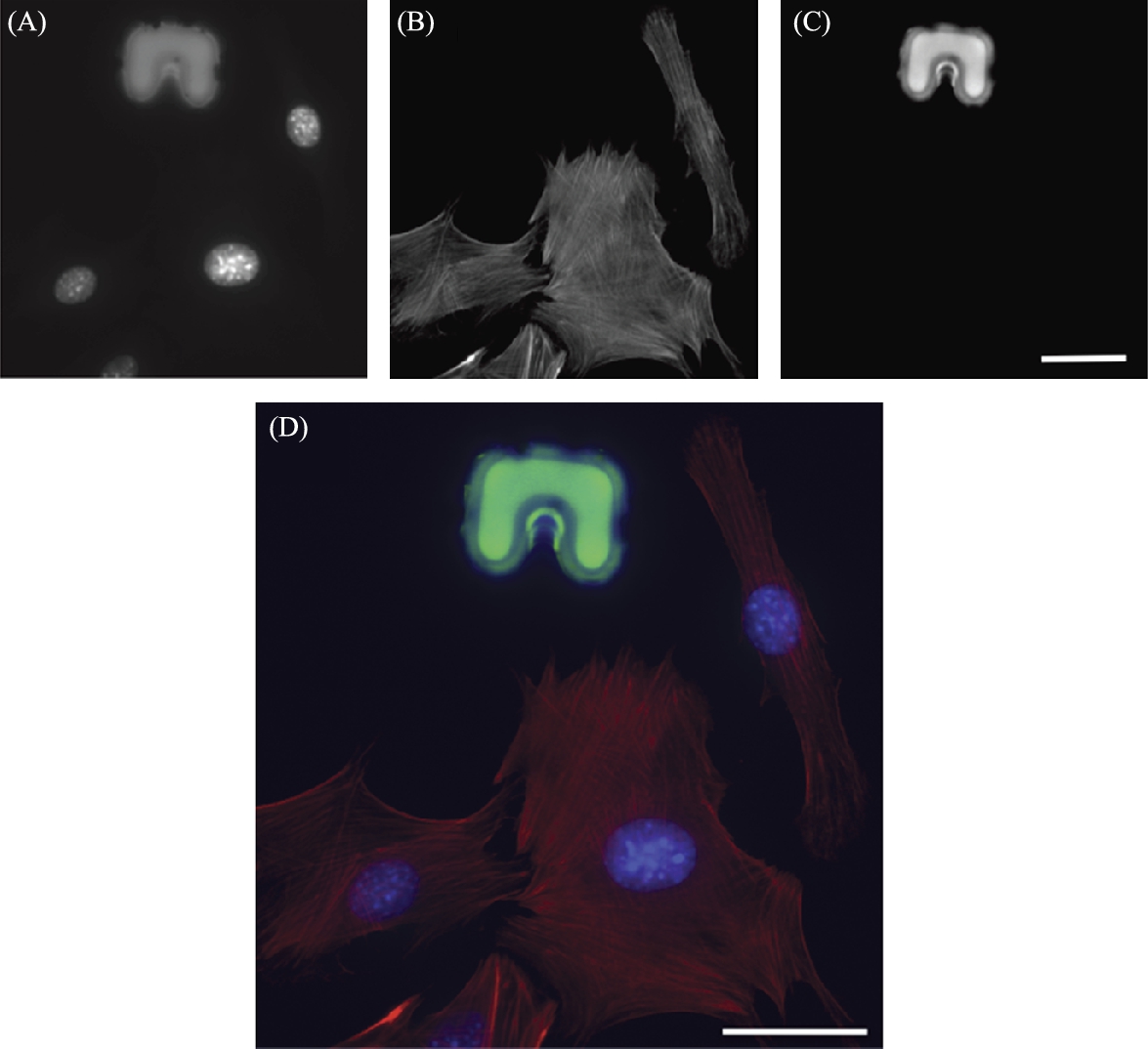
The captured image of microtransporters under fluorescent light is entirely different from the transmitted light image, therefore a completely different tracking algorithm is applied. Since SU8 is an autofluorescent material near the blue region of the light spectrum, the material appears as a bright solid against a black background in the captured image (Fig. 9.6(C)).
The primary advantage of this system is that all non-fluorescent entities simply do not appear in the image. For instance, adherent neuron cells typically form an interconnected pattern across the entire field of view. Using fluorescent microscopy, the cells are optically filtered out of the image, leaving only the microtransporter and fluorescently tagged microbeads in the image. The image is first binarized at an appropriate threshold, and a blob tracking algorithm is directly applied to this image. The objects are tracked using particle size filters or characteristic moments (Fig. 9.5).
A secondary advantage of this using fluorescent microscopy is that color information may be applied to increase selectivity. In this work, microbeads are also doped with fluorophores. By choosing an appropriate combination of fluorescent tag and filter, the beads appear as a different color than the microtransporter, and CV algorithms can then be tuned to track beads and robots independently, even when in close contact. This tagging can also be applied to cell bodies. In Fig. 9.6, an example of confocal (fluorescence) microscopy is shown where three distinct color bands correspond to each object of interest. In this case, nuclei of the cells appear in the blue band Fig. 9.6(A), actin filaments appear in the red band Fig. 9.6(B), and robots appear in the green band Fig. 9.6(C).
9.4.3 Manipulation of microbeads
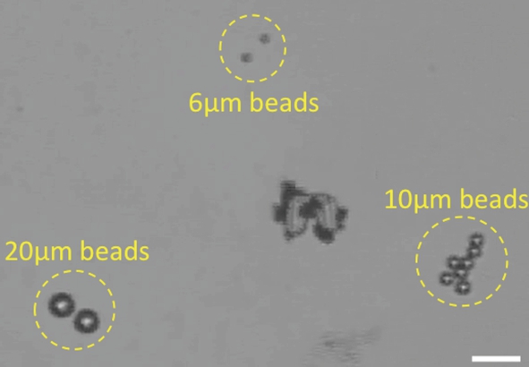
As an initial demonstration of the practical utility of the system, we demonstrate the mechanical manipulation of latex microbeads that are similar in size to several cell lines. One application that is desired by the single cell research is the collection and sorting of cells. Here, we use a dispersion of 6, 10, and 20 μm beads. The result of the sorting operation is shown in Fig. 9.7.
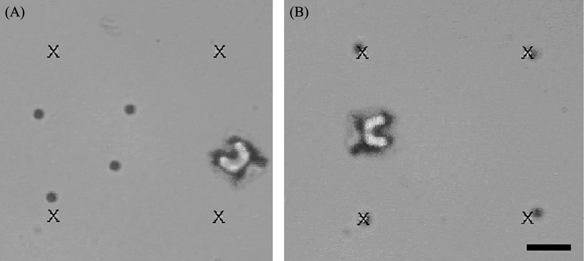
To demonstrate the accuracy of bead placement, we demonstrate the placement of microbeads at prescribed positions (Fig. 9.8). Four 10 μm were positioned on the corners of a virtual square. The challenges of viscous interactions between the robots and beads are present after placement as well before positioning. Thus, beads must be initially placed slightly past the markers, so that the robots pull the beads to the correct position as the robot is drawn back. Further, once a bead is placed, it is important to avoid traversing closely to the bead due to hydrodynamic interactions. There are two additional challenges of bead placement. Microbeads experience Brownian motion, which causes small long term changes in displacement. Also, localized convective flows are generated by heating from the microscope light sources and evaporation at the air/liquid interface.
9.4.4 Manipulation of cells
Latex microbeads are useful to study the manipulation tasks because the geometry, chemistry and surface interactions are highly uniform and predictable. Also, the beads may be stored for long terms and concentrations are simple to calculate. On the other hand, experiments with cells present several complications. Cells require culturing that takes days to weeks, the biochemistry is highly variable, the cells must be manipulated in buffer solution that sustain the viability, or at least the physical envelope of the cell. The greatest challenge with mechanically manipulating single cells is controlling the interactions of the cells with the substrate. For instance, erythrocytes (red blood cells) are highly adherent to glass slides. Thus, the challenges for individual manipulation of certain cell lines are greatly amplified. Here, we demonstrate the manipulation of three types of cells with varying sizes.
9.4.4.1 Yeast cells
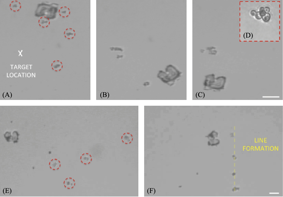
As an initial example, we manipulate budding yeast cells. The cells are diverse in size depending on the degree of budding, with the smallest individual cells measuring roughly 3–4 μm in diameter. In Fig. 9.9(A)–(C) we demonstrate gathering cells from a region into a closely packed group. In Fig. 9.9(E)–(F) we form an evenly spaced row of various sizes of yeast cells.
9.4.4.2 Mouse embryonic stem cells
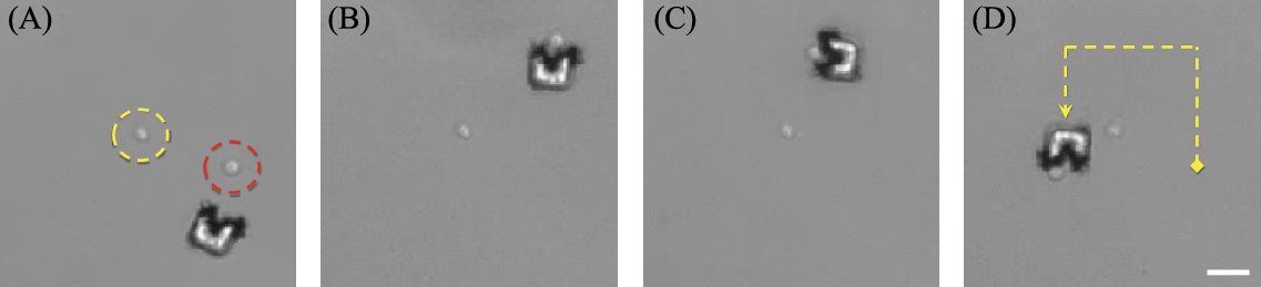
As an additional example of mechanical cell manipulation, we loop a mouse embryonic stem cell around a piece of glass debris (Fig. 9.10). The robot design becomes highly influential on the technique used to transport such cells. Whereas smaller cells such as yeast cells are easily trapped in the ‘cup’ of the transporter, larger cells such as the mouse embryonic stem cells tend to be pushed in front of the robot while being stabilized by the two arms of the cup-like shape. The cells used in this example were prepared in surfactant such that the adhesion between cells and substrates was moderate. Some cells tended to form adhesions with the substrate and the robot, but other cells were free of adhesive properties. This variability is representative of the challenges of handling individual cells. For each cell type and preparation, there may be significant variation in the interaction between the robot and the cell. As such, the application of data regarding manipulability across different cell lines and preparations may not hold.
9.4.4.3 Neuron transport
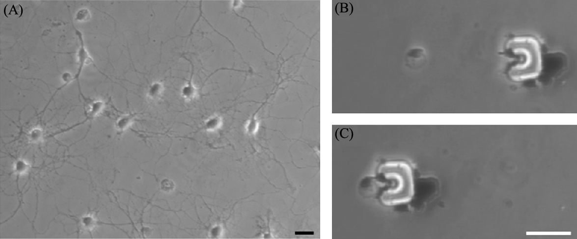
We detach cultured neurons from the surface by trypsinizing them in a solution (CMF-HBSS containing 0.5 mM EDTA and 0.05% trypsin) for 10 min at room temperature. Trypsin cleaves axons and dendrites and harvested cells change their morphology by taking a ball shape. Their dimensions vary from 10 to 30 μm. Cells are transferred onto another cover slip using a micropipette and microtransporters are released into the same fluid.
A microtransporter/target cell pair is selected and a path is planned for the manipulation task (Fig. 9.12(B)). When the transporter is in close proximity, the cell starts to move due to fluidic effects (Fig. 9.12(C)). We successfully release the target cell by moving the transporter in the opposite direction without changing its orientation. Adhesion between cells and transporters is observed, but this does not prevent release due to the shape of the robot and surface properties of trypsinized neurons.
9.4.5 Automation of single microrobots
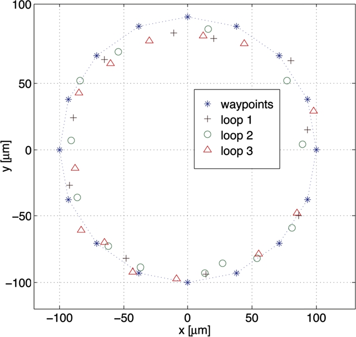
To demonstrate the repeatability of the tracking and control algorithms, we drove a microrobot along a circular trajectory in a series of three continuous loops. The data from this demonstration is presented in Fig. 9.11. The robot tends to correctly inscribe the waypoint paths since the destination waypoint is chosen to be two points ahead of the current position as each successive waypoint is approached.
9.4.6 Automated manipulation using bright field microscopy
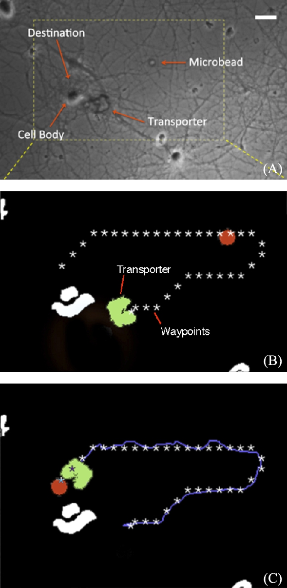
Automated manipulation of cells or microbeads can be performed using bright field microscopy; however, for manipulation of cells there are drawbacks to this technique. In Fig. 9.4, tracking is achieved by ensuring a workspace clear of debris and obstructions. Such a workspace cannot be achieved when culturing adherent biological cells for at two reasons. Firstly, the cells are harvested and scattered on the substrate during culturing, and there is little control over the dispersion and location of cells. Secondly, at least in the case of neurons, the cells must be in close proximity to proliferate. This can be seen in Fig. 9.13(A). The cell bodies and dendrites, which are of similar length scale to the microrobot, interfere with tracking algorithms designed for bright field microscopy. For this reason, tracking in fluorescence is a necessary solution.
9.4.7 Automated transport of chemically doped microbeads
An image of plated neurons cells is expanded into an appropriate configuration space using a thresholding and dilation routine. Neurons imaged with bright field techniques generally appear as a darker cell body surrounded by a lighter halo. The darker cell bodies are selected with thresholding, which results in a binarized map of obstacles. Noise is removed from the image with a particle size filter, and the identified obstacles are further dilated to ensure that robots do not collide with cells. The white blobs in Fig. 9.13(B) show the location of neuron cell bodies. The map of obstacles is then used in subsequent automation using fluorescent microscopy.
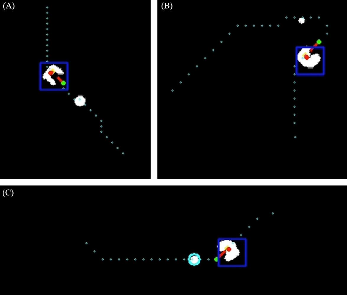
Although the position of the goal (the neuron) is fixed in this work, movement of the microbead should be taken into account in the path-planning algorithm. At this scale, non-contact interactions between the robot and the bead can be significant [14]. These interactions can be difficult to predict if the robot passes close to the bead while orienting itself for the approach and capture. Therefore, to make the system robust, the microbead should be tracked as it is approached, so that the path can be updated as required. After capture of the bead, sudden changes in orientation should be avoided so that the bead is not inadvertently lost.
When automating the delivery process, it is necessary to carefully consider methods for robust, repeatable capture and release of microbeads. Bead size for transport is an important design consideration for the microrobot. The U-shaped transporter used in this work enables caging and centering of microbeads such that they will not slip to the sides during transport (Fig. 9.14). Height is an equally important design consideration, since beads that are too small or too large may flow under or over the microrobot.
To ensure smooth delivery of the bead, we used a dual glass slide configuration. The microtransporter and bead operate on the lower surface of the setup, while the slide with adherent neurons is inverted above the microrobot and bead. The 30–50 μm gap between these two surfaces is large enough to allow smooth operation of robot without impinging directly on cells, yet close enough to image the robots and neurons in the same focal plane. There are additional fluidic benefits to this configuration. Firstly, diffusion of chemicals occurs in a two-dimensional slice rather than in a hemisphere, the effect of which is a greater localized chemical concentration. Secondly, convective effects are greatly reduced due to the enclosure.
9.4.8 Chemical transport
Controlled delivery of drugs or chemicals at the scale of the individual cell is a significant challenge. Encapsulation and transport of chemicals in microbeads has been widely studied, mainly as a technique for the distribution and extended release of pharmaceuticals [26]. Hydrogels, porous microspheres, and polymeric microbeads are all candidate technologies for the delivery of drugs to individual cells, however, PLGA microspheres stand out as the most appropriate technology for a variety of reasons.
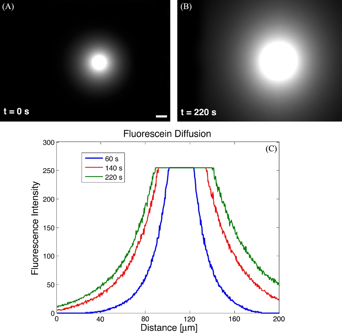
The time-release profile of chemicals is the primary selection criteria for drug delivery to individual cells. At the short end of the time scale, the experimental setup for automated microbead delivery typically requires from several seconds to a few minutes for the initial preparation of robots, microbeads and cells. On the other end of the time scale, individual cells may require tens of minutes to hours to respond to localized chemical changes in the environment. Hydrogels and porous microbeads typically release the bulk of encapsulated chemical within a few seconds to a few minutes, and therefore are not the best selection for chemical transport. PLGA beads exhibit a chemical burst over the first several hours of submersion, and are therefore better suited for microrobotic transport. Additionally, the microbeads are biocompatible, easily stored over extended time periods, and may be custom-made with standard lab equipment.
To visualize the initial release of chemical, a high concentration of fluorescein was encapsulated within microbeads. These beads were released on a glass slide and covered with a second slide, such that the diffusion occurs in a thin two-dimensional slice. The thickness of the slice is identical to the experimental setup used for neuron transport. The quasi-two-dimensional slice is helpful not only for concentration and localization of chemical, but also for the reduction of convective effects that are typically encountered due to non-uniform heating and evaporation. Fig. 9.15 shows the diffusion of chemical from the bead to the surrounding media.
9.5 Multirobot manipulation
Simultaneous control of multiple magnetic microrobots would offer significant benefits. By parallelizing operations, cells could be sorted or manipulated more quickly enabling higher throughput, microrobots could cooperatively transport objects, and varying chemical cues could be delivered simultaneously. As demonstrated in prior work, individually addressing magnetic robots is challenging because magnets respond similarly in a global field. Khalil et al. [27] controlled a cluster of 100 μm diameter paramagnetic microparticles to manipulate microstructures in a plane for microassembly. Multiple microparticles are manipulated together to push non-magnetic microstructures into a desired position. While multiple microparticles are manipulated, all the particles move in the same general direction and microparticles are not individually addressable. Strategies for transport of passive payloads using a team of homogeneous robots controlled by global inputs are discussed by Becker et al. [28].
Heterogeneous teams of magnetic microrobots generate different resultant forces under the same global field. Diller et al. [29] used a team of microrobots which are geometrically different but had similar effective magnetization, which resulted in different rotational inertia and therefore angular acceleration. Position control of 3 robots, each having dimensions less than 1 mm, is demonstrated; however, the motion of the robots is coupled and arbitrary trajectories are not possible. Cheang et al. [30] demonstrated control of 2 geometrically similar and magnetically heterogeneous microswimmers using a global rotating magnetic field. By balancing the applied magnetic torque and the hydrodynamic torque, simultaneous control of two microswimmers moving in opposing directions with arbitrary speeds can be achieved. Mahoney et al. [31] demonstrated control of two helical microrobots using robots with different magnetization and friction such that different forward swimming speeds result from the same magnetic field rotation frequency. The direction traveled at a given time step is the same but the velocity is different, which allows trajectories of the same shape but different size to be achieved. In these three methods, two microswimmers cannot swim in the same direction at the same velocity because the robots are heterogeneous.
Specialized printed circuit boards have been used to manipulate local magnetic fields on a surface to control multiple microrobots. Pelrine et al. [32] used layers of parallel and perpendicular traces on a printed circuit board to manipulate mm-sized magnetic robots. The current through the traces generate a local magnetic field, by varying the current through the traces the position of the robot is controlled. Cappelleri et al. [33] used microcoils on a printed circuit board to control multiple magnetic microrobots by affecting the local magnetic field. Planning and control algorithms for multiple microrobots on a planar system controlled by these microcoils are discussed by Chowdhury et al. [34]. Pawashe et al. [35] used a surface with electrostatic pads to selectively brake magnets and prevent them from moving while allowing the manipulation of other magnets away from the pad. These brakes are in fixed locations and the allowable trajectories are dominated by the position of the pads.
Apart from electromagnetic coils, mobile permanent magnets have also been used to control magnetic microrobots. Nelson and Abbott [36] demonstrated the ability to manipulate two magnetic devices by manipulating a single rotating magnetic dipole around the workspace. Converging, diverging and similar trajectories are achieved by exploiting the different magnetic field and field gradient at various locations around the magnetic dipole.
We demonstrate the ability to manipulate two identical magnets with globally applied fields using a system of four stationary electromagnets placed with the coils perpendicular to the plane, Fig. 9.16. By utilizing the spatially varying magnetic field gradients close to the coil and linearly superimposing the magnetic fields, it is possible to achieve different forces on identical magnets at close proximity; this allows independent trajectories to be executed simultaneously without the added complexity of heterogeneous robots. This approach differs from previous work in that the magnetic devices being manipulated have identical geometry and magnetization without the use of a specialized substrate. Additionally, we take advantage of spatial variations in the magnetic field gradient of four stationary electromagnetic coils controlled using variable current. We consider planar manipulation applications where the magnetic robots are restricted to the xy-plane. We present a mathematical model and dynamical simulation to demonstrate the ability to control two identical magnets along different trajectories. As a proof-of-concept, this control scheme is implemented on an experimental system for the manipulation of millimeter-sized disk-shaped magnetic robots. We show that magnetic robots can be simultaneously driven at various locations with the same velocity, as well as along differing trajectories.
 , illustrating the different forces exerted at different locations in the workspace. Reprint from [19].
9.6 Problem formulation
9.6.1 Background
A force is exerted on a ferromagnetic particle with a magnetic dipole moment, ![]() , when in the presence of a magnetic field,
, when in the presence of a magnetic field, ![]() . The magnetic field generated by a current loop can be derived by the Biot–Savart equation:
. The magnetic field generated by a current loop can be derived by the Biot–Savart equation:
where I is the current, ![]() is the permeability constant for air,
is the permeability constant for air, ![]() is the unit vector from the coil wire segment to the point of interest, and a closed loop integral is taken around the entire current loop, C, for each segment ds. This field exerts a force,
is the unit vector from the coil wire segment to the point of interest, and a closed loop integral is taken around the entire current loop, C, for each segment ds. This field exerts a force, ![]() , on a ferromagnetic particle given by
, on a ferromagnetic particle given by
The value for the magnetic dipole moment of the permanent magnet, ![]() , depends on material properties and geometry of the magnet.
, depends on material properties and geometry of the magnet.
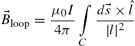
Four independently controlled electromagnetic coils are positioned such that the axes of the coils lie on the xy-plane with one pair of coils facing each other along the x-axis and the other pair of coils facing each other along the y-axis, Fig. 9.17(A)–(B). The xy-plane, where ![]() , is the plane on which the permanent magnets are manipulated.
, is the plane on which the permanent magnets are manipulated.
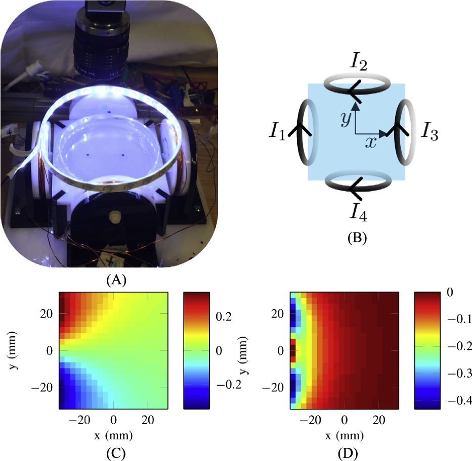
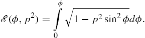
The magnetic field for the xy-plane at ![]() is computed using the Biot–Savart equation (9.4) for a circular loop with radius R, [37],
is computed using the Biot–Savart equation (9.4) for a circular loop with radius R, [37], ![]() :
:
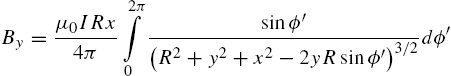
where ![]() is the variable of integration around the circular coil and is integrated around the full circle from 0 to 2π. This is summed over each coil. The solution of these integrals can be written in terms of incomplete elliptic integrals:
is the variable of integration around the circular coil and is integrated around the full circle from 0 to 2π. This is summed over each coil. The solution of these integrals can be written in terms of incomplete elliptic integrals:
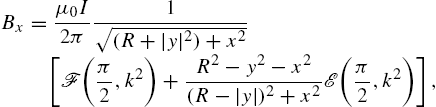
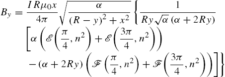
where ![]() ,
, ![]() , and
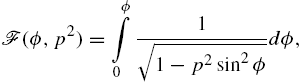
, and ![]() in the incomplete elliptic integrals
in the incomplete elliptic integrals ![]() and
and ![]() of the first and second kind, respectively,
of the first and second kind, respectively,
These expressions are used to compute the force and torque exerted on a magnet.
The magnetic torque, ![]() , is calculated by
, is calculated by
The torque acts to align the dipole of the robot with the field, ![]() . In this model, we assume that this reorientation occurs immediately for the robot, which is a permanent magnet, and the robot is always torque free [38,39]. The magnetic dipole moment,
. In this model, we assume that this reorientation occurs immediately for the robot, which is a permanent magnet, and the robot is always torque free [38,39]. The magnetic dipole moment, ![]() , is therefore expressed as
, is therefore expressed as
This is used with Eq. (9.5) and the expressions for the magnetic field to compute the force exerted on the magnet.
9.6.2 Multirobot model
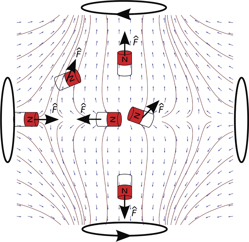
To achieve independent control, the field gradient must be non-uniform such that different forces can be exerted within the workspace. Fig. 9.16 shows the unit force vector field and corresponding streamlines lines generated by two opposing coils with equal and opposite current to illustrate the direction of forces, ![]() , applied at various locations within the workspace and the orientation of a magnet at different locations. Depending on the location of the magnets, it is possible to move magnets away from each other or towards each other to obtain a grasping motion on a payload.
, applied at various locations within the workspace and the orientation of a magnet at different locations. Depending on the location of the magnets, it is possible to move magnets away from each other or towards each other to obtain a grasping motion on a payload.
Eqs. (9.5)–(9.7) and (9.13) provide a mapping from the system inputs, currents, ![]() , to the forces,
, to the forces, ![]() , at specific positions,
, at specific positions, ![]() . This mapping, Φ, which is a function of the robot positions, takes the current inputs and maps it to force exerted on the robots,
. This mapping, Φ, which is a function of the robot positions, takes the current inputs and maps it to force exerted on the robots, ![]() .
.
For clarity, the system of four equations can be written as:
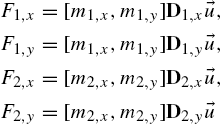
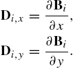
where ![]() is the
is the ![]() matrix form of the gradient of the magnetic field for the ith robot in the jth direction.
matrix form of the gradient of the magnetic field for the ith robot in the jth direction. ![]() is expressed as:
is expressed as:
The magnetic field at the position of the ith robot is written in matrix form as a sum of the magnetic field contribution from each of the four coils and is expressed as
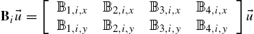
where ![]() is the current-normalized magnetic field, the first index is the coil number, the second is the ith robot location and the third is the component direction.
is the current-normalized magnetic field, the first index is the coil number, the second is the ith robot location and the third is the component direction.
To follow trajectories for two magnets in this planar configuration, the mapping, ![]() , is inverted to solve for currents required to exert a desired force given the robot positions,
, is inverted to solve for currents required to exert a desired force given the robot positions, ![]() . This inverse mapping cannot be derived explicitly because the force does not linearly depend on current, given that the orientation of the magnetic dipole,
. This inverse mapping cannot be derived explicitly because the force does not linearly depend on current, given that the orientation of the magnetic dipole, ![]() , is also a function of the current. The desired force is calculated by the feedback control algorithm and can be a function of the present and desired position, velocity, and acceleration of the magnet. A different formulation of the desired force is implemented in the simulation and experiments which are described in their respective sections.
, is also a function of the current. The desired force is calculated by the feedback control algorithm and can be a function of the present and desired position, velocity, and acceleration of the magnet. A different formulation of the desired force is implemented in the simulation and experiments which are described in their respective sections.
9.6.3 Approximate model
To simplify the computations, a point-dipole model is used to approximate the magnetic field generated by the electromagnetic coil, Eqs. (9.6) and (9.7). The magnetic field generated by a coil with radius R centered at ![]() , oriented with its axis along the y-axis, with a current I computed by the point-dipole model is given by
, oriented with its axis along the y-axis, with a current I computed by the point-dipole model is given by
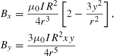
where ![]() is the distance from the center of the coil.
is the distance from the center of the coil.
Far away from the coil, ![]() , the magnetic field computed by the exact solution using elliptic integrals converges to the point-dipole model. Close to the coil, Fig. 9.17(C)–(D) compares the discrepancy in the direction and magnitude of the magnetic field near one coil of radius 25.5 mm positioned at
, the magnetic field computed by the exact solution using elliptic integrals converges to the point-dipole model. Close to the coil, Fig. 9.17(C)–(D) compares the discrepancy in the direction and magnitude of the magnetic field near one coil of radius 25.5 mm positioned at ![]() to mimic coil 1 in the experimental setup. The plot region represents the 60 mm square workspace centered at
to mimic coil 1 in the experimental setup. The plot region represents the 60 mm square workspace centered at ![]() , which is the center of the four coils. As expected, close to the edge of the coil, the angle and magnitude discrepancy is the greatest, and is relatively small at the center of the workspace.
, which is the center of the four coils. As expected, close to the edge of the coil, the angle and magnitude discrepancy is the greatest, and is relatively small at the center of the workspace.
9.7 Simulation
Control of the position of 2 magnets using the four coil system is first demonstrated in simulation. The magnetic field generated by the coils is modeled as a point-dipole using Eq. (9.17). The force exerted at each magnet is computed using Eq. (9.14).
The equations of motion consider the force exerted on each robot from the electromagnetic coil and a drag force. Inter-magnet forces are not included because the electromagnetic coils are unable to pull apart magnets once they have attached to each other. Therefore, the trajectories planned ensure a distance between the magnets such that the interaction force between magnets is small and negligible compared to the force exerted by the electromagnetic coils. To simulate the magnets floating, the drag force is modeled as quadratic drag, where the force is proportional to the square of the velocity of the robot,
where ρ is the density of water, ![]() is the drag coefficient, A is the cross-sectional area of the object, and v is the velocity of the magnet. For simplicity, the drag force is calculated using the model for a sphere moving in a fluid. A drag coefficient of 0.47 is used and the area is modeled as the cross-sectional area of a sphere with diameter 2 mm. This is likely an overestimate of the drag on a flat plate, because the drag on a sphere would be greater; additionally, the plate is at an air–water interface as opposed to submerged fully in water. Inertial forces are observed in the experiments, and therefore quadratic drag is used. When the electromagnets switch from on to off, the magnet continues to drift for a short but perceivable period of time. The Reynolds number in simulation is on the order of 100.
is the drag coefficient, A is the cross-sectional area of the object, and v is the velocity of the magnet. For simplicity, the drag force is calculated using the model for a sphere moving in a fluid. A drag coefficient of 0.47 is used and the area is modeled as the cross-sectional area of a sphere with diameter 2 mm. This is likely an overestimate of the drag on a flat plate, because the drag on a sphere would be greater; additionally, the plate is at an air–water interface as opposed to submerged fully in water. Inertial forces are observed in the experiments, and therefore quadratic drag is used. When the electromagnets switch from on to off, the magnet continues to drift for a short but perceivable period of time. The Reynolds number in simulation is on the order of 100.
A trajectory with waypoints defined by time, desired position, velocity, and acceleration is pre-computed. A PD controller with a feed forward term is used. The controller is updated at 100 Hz and the position of the robot is propagated between updates as a result of the current through the coils. At each controller update, a numerical solver is used to calculate the currents required to achieve the desired force at the present position of each robot by solving the system of four equations (9.14). MATLAB is used to simulate the system and the numerical solver function vpasolve is used to compute solutions to the system of equations (9.14). The differential equation solver function ode45 is used to calculate the position of the magnet as a result of the applied force.
Fig. 9.18 shows a simulated trajectory where one robot is held at coordinate ![]() and the other travels between
and the other travels between ![]() to
to ![]() . This example trajectory is used to illustrate our control strategy because holding one magnet still while moving another magnet within the same workspace is challenging using stationary electromagnetic coils.
. This example trajectory is used to illustrate our control strategy because holding one magnet still while moving another magnet within the same workspace is challenging using stationary electromagnetic coils.
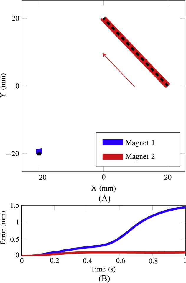
A fast update rate is needed because there can be high spatial variation in the magnetic field gradient causing changes in velocity as the magnet moves through space. Moreover, by updating the desired position to the next waypoint when the magnet position is within a certain bounding distance, as opposed to temporally prescribing the trajectory, can reduce position error for more complicated trajectories or when position errors are large. This position based waypoint update policy is implemented in the experimental system.
9.8 Multirobot experimental results
Due to the sensitivity of the magnets to small changes in the magnetic field, small currents can generate rotation and translation of the robot. The applied field magnitudes are 10–400 μT. This is on the order of magnitude of earth's magnetic field as evident by the consistent reorientation of the magnets when no current is applied. This causes a bias in the orientation of the magnet. Therefore, the expression for the magnetic dipole moment, expressed previously by Eq. (9.13), is written as the sum of the applied magnetic field by the coils, ![]() , and earth's magnetic field,
, and earth's magnetic field, ![]() :
:
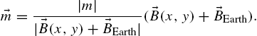
The magnitude and direction of earth's magnetic field is empirically derived as ![]() in the fixed frame of the workspace.
in the fixed frame of the workspace.
Waypoints are precomputed for each trajectory, with each waypoint defining a desired position, velocity and acceleration. The control sequence updates the desired position, velocity and acceleration to the next waypoint once the magnets are within a threshold radius from the desired waypoint. A threshold radius of 1.5 mm is used on the magnets that are moving along trajectories in the experimental results in Figs. 9.19 and 9.20.
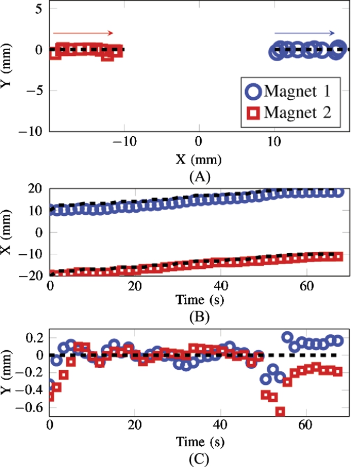
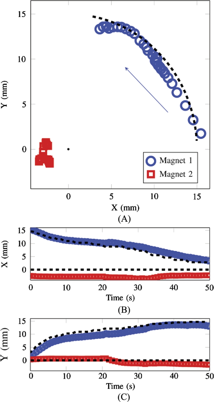
A unique feature of this system is the ability to exert the same forces on magnets at different locations so that magnets can move with the same velocity in addition to being able to move along differing trajectories. Fig. 9.19 shows a trajectory where both magnets are moving at the same velocity in the positive x-direction. Fig. 9.20 shows a trajectory where one robot is held stationary as the other is moving in a counter-clockwise arc with a radius of 15 mm.
9.9 Conclusion
We described the construction and operation of micron-sized, biocompatible ferromagnetic microtransporters driven by external magnetic fields. The five-coiled, compact actuation system is designed for rapid integration with existing microscopes. We use a real-time visual tracking algorithm for tracking transporters and target objects. Tracking algorithms are described for tracking robots and beads using bright field as well as fluorescence microscopy. This information is used to implement fully automated manipulation of microbeads. We also demonstrate the transport of rat hippocampal neurons and microbeads with teleoperation. In a fully automated integration of these elements, microbeads are positioned at target locations by individual neurons for delivering drugs to cultured neurons.
By integrating biodegradable PLGA microbeads with magnetic microrobots, we showed the feasibility of delivering chemicals locally and engineering more in vivo-like microenvironments in vitro. Polymeric microbeads have been established as an effective means of encapsulating and delivering drugs. Localized complex molecular gradients can be created at target locations by positioning multiple beads in the same vicinity [40]. As a result, the combinatorial effect of multiple growth factors and therapeutic agents on living cells can be analyzed. This capability has important applications in stem cell differentiation and cancer studies. Furthermore, their design may be specifically tailored for customized time-based release or even release in response to environmental or other external triggers [41]. Using this technology, drugs can be delivered at pre-determined times and with specific doses.
We also presented a theoretical framework to achieve independent position control of 2 identical magnets in a planar system. Our method uses the spatially varying gradient of the magnetic field close to the electromagnetic coil and the superposition of the fields independently generated by several stationary electromagnetic coils. We analyzed this method in simulation and experiment in order to show that independent forces can be applied on each robot. Experimental results demonstrated trajectory following using visual feedback. This control scheme has potential applications in micromanipulation for automated high-throughput biological experiments and use inside microfluidic channels for analysis and microassembly.