
Obstacle avoidance for bacteria-powered microrobots
Hoyeon Kim⁎; Anak Agung Julius†; MinJun Kim⁎ ⁎Southern Methodist University, Dallas, TX, United States
†Rensselaer Polytechnic Institute, Troy, NY, United States
Abstract
For practical applications that involve microrobots there are several control related challenges. These challenges are often alleviated by constructing ideal environments, which are devoid of potential disturbances that can affect performance. However, in less idealistic working spaces where obstacles exist, microrobotic navigation algorithms must account for these objects. An autonomous control system will be more efficient than manual control to avoid these obstacles. In addition, the autonomous navigation will widen the potential application of microrobots, as autonomous control can supply the optimal motion control depending on the situation. In this chapter, we introduce a static obstacle avoidance algorithm for bacteria-powered microrobots. A bacteria-powered microrobot (BPM) is a hybrid robotic system consisting of an inorganic SU-8 microstructure with bacterial carpets, in which massive arrays of biomolecular flagellar motors work cooperatively. Our obstacle-avoidance method is based on a BPM's response to electric fields; the negatively charged bacteria enable the BPM to follow the electric field lines. In this chapter, the constraint elements to develop the obstacle avoidance method are discussed and demonstrated by experiments with simulation results. In the suggested approach, the methods, such as potential function and configuration-space, popular in macroscale robotics, are applied to microscale robotics. We describe the feasibility of the proposed obstacle avoidance approach through experiments and compare these data with simulation results.
Keywords
Navigation; Obstacle avoidance; Motion control; Microrobot
5.1 Introduction
Microrobots have shown significant potential to conduct microscale tasks such as drug delivery, cell manipulation, microassembly, and biosensing [1–3] using manual control. For instance, the application of targeted delivery was demonstrated using magnetotactic bacteria under DC magnetic field gradients [4]. Other research groups have also explored microrobots for transporting target objects such as cells and chemicals using magnetic field [5,6]. In addition to targeted delivery, microgrippers have been developed for microrobots using micro-electro-mechanical systems [7], a technology which can be used to improve functionality of microrobots [8–10]. In order to achieve motion control, the kinematic models of developed microrobots have been studied [5,11]. The biological and non-biological microrobots have been navigated by autonomous motion planning [12–14]. These technologies are based on feedback control based on vision systems.
In this chapter, the obstacle avoidance approach is introduced and demonstrated using bacteria-powered microrobots (BPMs) which are actuated by biomolecular motors of live bacteria. The attached bacteria mobilize the inorganic substrate which, without bacteria, is not controllably movable under any external stimuli. The live bacterium, S. marcescens, has a net negative surface charge and cannot be controlled by magnetic coils, as it exhibits no magnetotaxis. BPMs can be actuated by applying external stimuli such as specific wavelengths of light, electric fields, and chemical gradients [15–18]. Feedback control has been thoroughly demonstrated to guide the BPMs to desired positions in previous work [19]. BPMs have been also employed as mobile phenotype biosensors and can be chemically manipulated to enhance steering [19]. This chapter focuses on developing a navigation algorithm using an obstacle avoidance method which we demonstrate by navigating BPMs in cluttered environments using different parameters in the algorithm [14,20].
To develop the motion control of BPMs for obstacle avoidance in microfluidic environments, there are two primary constraints that affect the motion control. First, the electric field deforms locally around the corners, resulting in distorted BPM trajectories, similar to the particle motion around 90° L-channels observed in a galvanotaxis system [21]. The other constraint is the inherent self-actuation motion of BPMs. Self-actuation of BPMs is not controlled by the external control system. To resolve these issues, we developed and carried out an obstacle avoidance method using a kinematic model of the BPM [16]. This kinematic model predicts the BPM's position and its response to the control input. Thus, our obstacle avoidance algorithm considers these constraints to prevent BPMs from colliding with obstacles.
We review the kinematic model of BPMs and its feasibility for obstacle avoidance. Then, we compare the simulation of the kinematic model with experimental data. The next section describes the critical factors for the obstacle avoidance approach and introduces our algorithm; the experimental system and procedure are also presented. The last section demonstrates the suggested approach in several experiments with respect to different environments and parameters, along with a comparison with simulation results.
5.2 Kinematic model of a bacteria-powered microrobot
In low Reynolds number fluid environments, the hydrodynamics of the swimming motion used by bacteria, such as that of Escherichia coli and S. marcescens, has been of great interest to a number of research groups [22–24]. Swimming bacteria move by hydrodynamic force that is generated by the helical motion created by a bundle of rotating flagella [25–27]. In order to propel microrobots in microfluidic environments, a strong translation force is required, such as the collective propulsion of flagella from a myriad of bacteria [28]. In our system, a BPM is a hybrid microrobotic system which consists of an artificial body (SU-8 microstructure) and a biomolecular actuator (bacterial carpet of S. marcescens). The bacterial carpet generates the resultant thrust under the structure by the random reversal of flagellar rotation [26]. The bacterial carpet is a monolayer of unpatterned swarming bacteria. An SU-8 microstructure is created using general photolithography. Then swarming bacteria cultured on an agar plate are blotted onto these microstructures, which are still attached to the glass substrate; the bacteria on the agar plate will adhere to the surface of the microstructure, creating the bacterial carpet. The blotted structures are then released by dissolving the sacrificial layer (10% Dextran) between the SU-8 and the substrate [18]; once released, these untethered structures are referred to as BPMs. Without external stimuli, BPMs generally have an average velocity of 5 μm/s.
After blotting a microstructure with bacteria, self-actuation of the BPM can be observed without external control input. This motion is due to the fluid flow caused by the rotation of many flagella on the bacterial carpet. The motion of self-actuated BPMs can be represented by two separate velocities on the local axis and one angular velocity for the rotation of the BPM.
The distinct translational velocities can be expressed with respect to the x- and y-axis in the inertial coordinate frame in accordance with the center of mass. The inertial coordinate system follows the orientation of the BPM's body [15]. Hence, the translational and rotational velocity of self-actuation can be explained by


and where ![]() is the number of bacteria on the surface of the microstructure;
is the number of bacteria on the surface of the microstructure; ![]() and
and ![]() are the translational and rotational viscous drag coefficients, respectively;
are the translational and rotational viscous drag coefficients, respectively; ![]() is the vector of the ith bacterium in the body-fixed coordinate. The units of
is the vector of the ith bacterium in the body-fixed coordinate. The units of ![]() and
and ![]() are μm/(s⋅pN) and rad/(s⋅pN), respectively [16].
are μm/(s⋅pN) and rad/(s⋅pN), respectively [16].
According to the kinematic model, the translational velocities, ![]() and
and ![]() , are proportional to the mean of the propulsion forces,
, are proportional to the mean of the propulsion forces, ![]() . The propulsive force
. The propulsive force ![]() has an average of 0.45 pN for individual bacterium [22]. Unlike
has an average of 0.45 pN for individual bacterium [22]. Unlike ![]() , the parameters
, the parameters ![]() and
and ![]() are related to the quantity of attached cell bodies and each bacterium's respective orientation
are related to the quantity of attached cell bodies and each bacterium's respective orientation ![]() on the BPM. Hence,
on the BPM. Hence, ![]() and
and ![]() are greatly influenced by the self-actuated motion because the resulting force depends on the orientation of cell bodies, how much the orientation varies, and the general coverage of bacteria on the microstructure.
are greatly influenced by the self-actuated motion because the resulting force depends on the orientation of cell bodies, how much the orientation varies, and the general coverage of bacteria on the microstructure.
The propulsion contribution of cells to the self-actuation motion was experimentally examined with respect to the bacteria-attached region. By immobilizing bacteria within selected areas using UV light, it was determined that the regions with predominant momentum were at the edges of the BPM [18,19,29].
For BPM control, the negative charge of the cells, a characteristic innate to gram-negative bacteria, can be exploited to control cells using electric fields. Their behavior is comparable to electrons in electrophoresis. Therefore, as a DC electric field is applied to BPMs, electrokinetics will produce BPMs locomotion.
A component for electrokinetic actuation is added in a stochastic model from previous work [15]. Therefore, the BPM's position in the global coordinate system can be expressed as

where ![]() and
and ![]() are the control input voltages for movement in the x- and y-direction, respectively, and
are the control input voltages for movement in the x- and y-direction, respectively, and ![]() is the sampling time.
is the sampling time. ![]() represents the total electrophoretic force from the total charge of the adhered cells. The velocity of the BPM is proportional to the resultant magnitude of the applied two voltages. The BPM can immediately steer in any direction without inertial effects because inertial forces are negligible in low Reynolds number environments.
represents the total electrophoretic force from the total charge of the adhered cells. The velocity of the BPM is proportional to the resultant magnitude of the applied two voltages. The BPM can immediately steer in any direction without inertial effects because inertial forces are negligible in low Reynolds number environments. ![]() ,
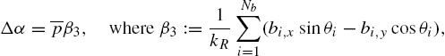
, ![]() , and Δα can be simplified as
, and Δα can be simplified as

Finally, we can approximate the motion of BPMs using a mathematical model (5.4) as a function of four property parameters, ![]() ,
, ![]() ,
, ![]() , and
, and ![]() , and the control input voltages. This model is implemented in our proposed algorithm. Furthermore, this stochastic motion model is useful in calculating the expected position of BPMs given an optimal control input generated using our obstacle avoidance approach. Through the kinematic model of the BPM, the trajectory can be determined by
, and the control input voltages. This model is implemented in our proposed algorithm. Furthermore, this stochastic motion model is useful in calculating the expected position of BPMs given an optimal control input generated using our obstacle avoidance approach. Through the kinematic model of the BPM, the trajectory can be determined by ![]() and
and ![]() continuously. Our proposed obstacle avoidance method determines the optimal input voltages
continuously. Our proposed obstacle avoidance method determines the optimal input voltages ![]() and
and ![]() in real time.
in real time.
In order to use the stochastic model for the position of BPMs with control inputs in our algorithm, the modeling parameters ![]() ,
, ![]() ,
, ![]() , and
, and ![]() should be validated. Using kinematic model equations (5.4), the real position data from experiments is compared with the calculated positions.
should be validated. Using kinematic model equations (5.4), the real position data from experiments is compared with the calculated positions.
First, the parameters ![]() ,
, ![]() , and
, and ![]() , which are related to self-actuation motion of a BPM, need to be estimated.
, which are related to self-actuation motion of a BPM, need to be estimated. ![]() is calculated by measuring the average angular velocity while only self-actuation motion is present (note that
is calculated by measuring the average angular velocity while only self-actuation motion is present (note that ![]() and
and ![]() in (5.4) have a different
in (5.4) have a different ![]() axis orientation during each sampling period). Then, the frame-by-frame x and y displacement values,
axis orientation during each sampling period). Then, the frame-by-frame x and y displacement values, ![]() and
and ![]() , at the ith and (
, at the ith and (![]() )th frame are computed from consecutive images. With these values,
)th frame are computed from consecutive images. With these values, ![]() ,
, ![]() are obtained from the inverse solution of the following matrix:
are obtained from the inverse solution of the following matrix:

After obtaining the parameters for self-actuation, the parameter ![]() for electrophoretic locomotion is determined by (5.7) under a control input voltage,
for electrophoretic locomotion is determined by (5.7) under a control input voltage,

In order to prove the kinematic model, the experimental data (blue triangles) from tracking [19] was compared with simulated position data (white dots) (Fig. 5.1). The electric field was applied from right (anode) to left (cathode) ranging from 1 to 10 V/cm. The simulated motion (dashed white lines) was almost same with the experimental position. The error distance between the actual BPM positions and the simulation positions is less than 3.5 μm, and the average is 0.73 μm during 70 s. This result validates the kinematic model for the experiment and simulation.

For obstacle avoidance simulations, we calculated the position of a moving BPM from the motion model using the experimental data. Similar to calculating the BPM's position, ![]() was calculated first and the rest of the parameters,
was calculated first and the rest of the parameters, ![]() ,
, ![]() , and
, and ![]() , were subsequently determined for the full duration of the video. The extracted parameters were used for the BPM in obstacle avoidance algorithm simulation. The estimation calculations and simulation results can be found in the results section.
, were subsequently determined for the full duration of the video. The extracted parameters were used for the BPM in obstacle avoidance algorithm simulation. The estimation calculations and simulation results can be found in the results section.
5.3 Obstacle avoidance approach
5.3.1 Considerations for control
Before developing an obstacle avoidance approach for BPMs, we have to take into account several factors. First, the BPM's inherent self-actuation motion is not controllable by external electric fields and significantly increases the probability of obstacle collision even under the control of an electric field. If ![]() ,
, ![]() , and
, and ![]() , which determine the self-actuation motion in the model (5.1), (5.2), and (5.3), are extracted in the experiment, then the predicted location can be computed by the kinematic model and taken into account by the control input to avoid collision.
, which determine the self-actuation motion in the model (5.1), (5.2), and (5.3), are extracted in the experiment, then the predicted location can be computed by the kinematic model and taken into account by the control input to avoid collision.
Another parameter to consider is the experimental test area. To generate electric fields, two pairs of electrodes are placed at the opposing edges of the control area. However, the electric field generated from these electrodes can be significantly distorted by any obstacles present. To properly address this issue, we characterized an electric field around an obstacle using COMSOL Multiphysics.
The simulation results and the real trajectories of BPMs under the same electric field are demonstrated in Fig. 5.2 and Fig. 5.3. A 10 V/cm (the anode is to the left, and the cathode is to the right) electric field is present in Fig. 5.2(A). The trajectories of charged particles at different positions were simulated. Obstacles in the simulation were considered as insulators. The electric field was distorted near the corners of the obstacles. The strength of the electric field is also weaker in the areas close to the obstacles. The charged particles had a mass of ![]() and a charge of
and a charge of ![]() for COMSOL Multiphysics simulation. They could be driven by electrophoresis as they moved along the flow of electric field as shown in Fig. 5.2(A). As the particles approached the distorted electric field concentrated around an obstacle, particles whose trajectory did not cross the obstacle continued to move horizontally towards the positive electrode. However, particles which started directly to the right of the obstacle stopped adjacent to the obstacle area due to the absence of any electric potential energy gradient. Particles that passed by the first corner of the obstacle also had affected trajectories, even though they had clear space ahead to pass; this was due to the distorted electric field. As a result, the directions of particles were different from the desired control direction (see Fig. 5.2(A)). The smaller the distance between the particle and the obstacle, the larger the difference between the simulated trajectory and directional input. This phenomenon is confirmed by comparing this simulation to experimental results (see Fig. 5.2(B)). The BPMs which exhibited very weak self-actuation were exposed to the electric field of the same magnitude from the simulation. Similar to the first case, the BPM stopped in front of the obstacle. However, in the second case, the BPM moved to the desired direction around the obstacle because it was out of the range of the electric field distortion.
for COMSOL Multiphysics simulation. They could be driven by electrophoresis as they moved along the flow of electric field as shown in Fig. 5.2(A). As the particles approached the distorted electric field concentrated around an obstacle, particles whose trajectory did not cross the obstacle continued to move horizontally towards the positive electrode. However, particles which started directly to the right of the obstacle stopped adjacent to the obstacle area due to the absence of any electric potential energy gradient. Particles that passed by the first corner of the obstacle also had affected trajectories, even though they had clear space ahead to pass; this was due to the distorted electric field. As a result, the directions of particles were different from the desired control direction (see Fig. 5.2(A)). The smaller the distance between the particle and the obstacle, the larger the difference between the simulated trajectory and directional input. This phenomenon is confirmed by comparing this simulation to experimental results (see Fig. 5.2(B)). The BPMs which exhibited very weak self-actuation were exposed to the electric field of the same magnitude from the simulation. Similar to the first case, the BPM stopped in front of the obstacle. However, in the second case, the BPM moved to the desired direction around the obstacle because it was out of the range of the electric field distortion.


To verify the deformed trajectory around the distorted electric field, the diagonal electric field flow with a positive electrode at the bottom left and a negative electrode at the top right was applied. This simulation also verified the distortion of electric field around the obstacle through the trajectories of negatively charged particles (Fig. 5.3(A)). Similarly, some of particles stopped where a potential gradient was too small. In these cases, a small charged particle with the weight electron was used in simulation as explained above, and the trajectories were found to be different depending on the properties of particle in terms of size and charge. Experimentally, the BPM followed the electric field flow around the obstacle with diagonal voltage input. The amount of distortion of this electric field depended on the distance from the obstacle and the trajectory (Fig. 5.3(A)). The motion of the BPM between ![]() to
to ![]() deviated from the diagonal direction more than from
deviated from the diagonal direction more than from ![]() to
to ![]() (Fig. 5.3(B)). These two comparisons between simulation results and real experimental data confirm that the behaviors of charged particles and BPMs are similar for future simulation and calculation purposes. Given the non-intuitive movement of BPMs in close proximity of obstacles, it is favorable to avoid these uncontrollable areas where the electric field deformation can lead to large errors from the expected position.
(Fig. 5.3(B)). These two comparisons between simulation results and real experimental data confirm that the behaviors of charged particles and BPMs are similar for future simulation and calculation purposes. Given the non-intuitive movement of BPMs in close proximity of obstacles, it is favorable to avoid these uncontrollable areas where the electric field deformation can lead to large errors from the expected position.
The last factor for BPM obstacle avoidance control is related to kinematic constraints. Unlike a macroscale two-wheeled mobile robot, BPMs can move in any direction instantly without kinematic constraints. The motion of a BPM is a kind of holonomic system, like an omnidirectional mobile robot. The suggested obstacle avoidance method should take into account these factors to generate a controllable and safe motion planning for a BPM.
5.3.2 Proposed obstacle avoidance method
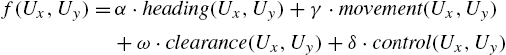
The suggested obstacle avoidance method incorporates all constraint factors. An objective function to enhance the controllability in the electric field is added to the objective function based on the dynamic window approach (DWA) [30]. Our alternative method searches the admissible control input at an instant position to maintain a suitable displacement to head towards the goal without any collisions. The control input is determined from four different functions: heading, clearance, movement, and control. In each function, the cost represents the quantity for each performance (such as moving direction toward a goal, collision check, large displacement, and controllability under electric field) with respect to searching control input, and is dimensionless after normalizing it to be in the range from 0 to 1. The derived input maximizes the sum of the cost values from these functions within the two-dimensional velocity search space.
Our proposed algorithm is established to facilitate the controllability of BPMs and to account for the deformation of the electric field in the region of insulating obstacles which can cause undesirable movement. The core function in our algorithm is the objective function which will produce a safe motion plan without collisions as follows:
where ![]() and
and ![]() are the searched voltage input that determines the electric field.
are the searched voltage input that determines the electric field.
The cost of the heading function represents the alignment of a BPM with the goal direction. However, it is difficult to determine a heading orientation of the BPM and adjust the orientation with electric fields. It also does not have any restrictions preventing change in any direction under an electric field. In order to quantify the cost value for all different moving directions, we used the inner angle ϕ, which is the angle between two predicted vectors. The first vector is the direction from the BPM's current point to the next point, and the second vector is the direction from the next position to the goal position. The angle is normalized as ![]() ; thus, the maximum possible value for ϕ will be 180° which means the BPM can move backwards.
; thus, the maximum possible value for ϕ will be 180° which means the BPM can move backwards.
Two control input examples for the cost of the heading function are illustrated (Fig. 5.4(A)). Using two different input values, each position in the next interval can be located where ![]() and
and ![]() indicate the predicted heading direction from the current location of the BPM, and
indicate the predicted heading direction from the current location of the BPM, and ![]() and
and ![]() represent the estimated goal direction from the next position. We can estimate the heading cost with respect to
represent the estimated goal direction from the next position. We can estimate the heading cost with respect to ![]() and
and ![]() which are the angles between
which are the angles between ![]() and
and ![]() , and between
, and between ![]() and
and ![]() , respectively. The inner angle is useful in determining which direction has change of heading angle, such as a straight line to the goal position. As a result, the internal angle
, respectively. The inner angle is useful in determining which direction has change of heading angle, such as a straight line to the goal position. As a result, the internal angle ![]() has a high cost for the heading function. The maximum value lies between 0 and
has a high cost for the heading function. The maximum value lies between 0 and ![]() , and it is expected that all input values on the same θ will have high values. However, the control velocities which are generated between
, and it is expected that all input values on the same θ will have high values. However, the control velocities which are generated between ![]() and
and ![]() have a low cost because in these cases the BPM moves away from the goal.
have a low cost because in these cases the BPM moves away from the goal.

The movement function helps us to find the control input which has a long movement of the BPM during sampling time. It is obvious that higher ![]() and
and ![]() are induced by a high voltage input. The cost of movement is given as
are induced by a high voltage input. The cost of movement is given as
where ![]() is the maximum movement from a maximum input voltage
is the maximum movement from a maximum input voltage ![]() on both axes for one interval. For BPMs to reach the goal position in a short time, the movement function extracts a voltage input which has a large displacement.
on both axes for one interval. For BPMs to reach the goal position in a short time, the movement function extracts a voltage input which has a large displacement.
Moreover, in order to prevent obstacle collisions from a control input value, the self-actuation of BPMs is taken into consideration with a clearance function. While a BPM shows self-actuation, we analyze the components for ![]() ,
, ![]() , and
, and ![]() . Afterwards, the expected position will result from the kinematic model (5.4) with the determined model parameters and each
. Afterwards, the expected position will result from the kinematic model (5.4) with the determined model parameters and each ![]() and
and ![]() at the present position. The possibility of a collision is calculated by the clearance function using the configuration-space (C-space) at the predicted position.
at the present position. The possibility of a collision is calculated by the clearance function using the configuration-space (C-space) at the predicted position.
The clearance function is utilized to evaluate the collision probability for a corresponding motion. In the proposed algorithm, the C-space is predefined first from the environment map by assuming that a BPM is a circular robot for which the radius is the maximum edge distance from the center of the BPM for collision check. Using the C-space, we can identify the occurrence of a collision with an obstacle at the predicted position. The self-actuated BPM could collide with the obstacle while it is controlled by the electric field. Thus, the clearance cost measures the shortest distance from occupied areas of the C-space considering movement of self-actuation. If the shortest distance between the BPM and the obstacles is within the possible range of movement from self-actuation, the clearance cost will be 0.
The control function focuses on driving the BPM to the desired direction using the generated electric field from its current position by placing the BPM on a path where it is affected by the electric field more efficiently and strongly. To get the cost of the control function, the computation of the intrinsic electrical potential field for the whole area is calculated during post processing before executing our algorithms. Then, the cost of the control function is used to find which control input in the possible velocity space drives the BPM to a high potential area where electric field distortion is minimal or nonexistent. Therefore, the control function measures the amount of controllability by calculating every 45° angle direction force under maximum electric field at the predicted position using ![]() and
and ![]() as follows:
as follows:

where ![]() is the maximum intrinsic potential field value.
is the maximum intrinsic potential field value. ![]() is the gradient of the electric field at the estimated position using
is the gradient of the electric field at the estimated position using ![]() and
and ![]() (Fig. 5.5). The layers of electric field around the BPM shown in Fig. 5.5(A) are a result of the computation of the intrinsic potential field. Area 1 is a distorted region where the gradient electric potential exists, and Area 2 represents a region with a uniform electric potential. In Area 2, the BPM is able to follow a control input with a high cost of the control function because it is not in any gradient potential field caused by a deformation of the electric field. The control function supplies information about the distortion of electric field lines when the BPM is driven by eight different input directions at given positions. Thus, the cost will be higher in areas where there is less electric field distortion. The resulting cost from the control function is described in Fig. 5.5(B). High control cost values are placed near π and −π. Therefore, the control function encourages the BPM move toward the closest local region in Area 2 in this example. Finally, the control function places preference for movements toward undistorted electric fields (e.g. Area 2) to minimize resultant displacements and desired control trajectory distortion.
(Fig. 5.5). The layers of electric field around the BPM shown in Fig. 5.5(A) are a result of the computation of the intrinsic potential field. Area 1 is a distorted region where the gradient electric potential exists, and Area 2 represents a region with a uniform electric potential. In Area 2, the BPM is able to follow a control input with a high cost of the control function because it is not in any gradient potential field caused by a deformation of the electric field. The control function supplies information about the distortion of electric field lines when the BPM is driven by eight different input directions at given positions. Thus, the cost will be higher in areas where there is less electric field distortion. The resulting cost from the control function is described in Fig. 5.5(B). High control cost values are placed near π and −π. Therefore, the control function encourages the BPM move toward the closest local region in Area 2 in this example. Finally, the control function places preference for movements toward undistorted electric fields (e.g. Area 2) to minimize resultant displacements and desired control trajectory distortion.

The objective of our algorithm is composed of four different functions that have particular purposes so that the chosen input can perform the optimal control motion regarding the constraints of the system and the characteristics of BPMs. The selected input voltage in the space of admissible voltages will be derived from the weighted sum of all these components in (5.8) after these components are normalized to [![]() ]. The selected control input has a maximum peak in (5.8) and the motion control input can be varied depending on the weighting of the parameters α, γ, ω, and δ that represent the contribution of each function in the resulting cost from the objective function.
]. The selected control input has a maximum peak in (5.8) and the motion control input can be varied depending on the weighting of the parameters α, γ, ω, and δ that represent the contribution of each function in the resulting cost from the objective function.
Therefore, the scheme computes the objective function integrating these four functions for all possible control inputs for the current position. We illustrate how to obtain the optimal control input in our proposed objective function (Fig. 5.6). When the position of the BPM and obstacles are indicated in Fig. 5.6(A), the resulting cost values for heading, clearance, movement, and control functions, respectively, are as in Fig. 5.6(B)–(E) at the given position of the BPM. Next, the result of the objective function was calculated by adding costs with different weight values as shown in Fig. 5.6(F). In this case, the parameters are 0.56, 0.5, 0.4, and 0.5 for α, γ, ω, and δ. Finally, the algorithm chooses the control input which has the highest peak value in Fig. 5.6(F). Until the BPM reaches its target destination, the obstacle avoidance algorithm will sustain an optimal velocity for the BPM in subsequent intervals which has a maximum cost for the objective function.

5.4 Motion under obstacle avoidance
5.4.1 Electric field control for BPMs
We used a microchannel composed of polydimethylsiloxane (PDMS) that contained obstacles in the workspace. Before PDMS was bonded to a glass substrate, the obstacles were fabricated first on the glass substrate using traditional soft lithography. We created 20 μm thick structures for obstacles with SU-8 2010 photoresist to prevent the BPMs from moving over them. After the obstacles were made, the glass substrate was bonded to the prepared PDMS chamber using oxygen plasma etching.
The control chamber was filled with a motility buffer containing 0.05% polyethyleneglycol (PEG). Two pairs of platinum wires were fixed in parallel positions with respect to the horizontal and vertical direction. Even though the platinum wire does not make residuals such as graphite electrodes, bubbles formed around the platinum wire. Therefore, DC electric fields were applied to the BPMs through agar salt bridges, using Steinberg's solution (0.7 mM KCl, 0.8 mM MgSO4⋅7H2O, 60 mM NaCl, 0.3 mM CaNO3⋅4H2O). Voltages were supplied via two power supplies.
The inorganic body of BPMs was fabricated using conventional photolithography with SU-8 negative photoresist. Before SU-8 microstructures were patterned on the glass slides, a water-soluble sacrificial dextran layer was added by a spin-coater [31]. We used a 7% dextran solution. The dispensed dextran layer was baked at 125°C. Then, the 3 μm thick layer of SU-8 2002 was coated on the dextran layer by spin-coating. A 32 μm × 30 μm rectangular square-patterned chrome mask was used for exposure. The film was dissolved in developer, leaving only the structures and the dextran sacrificial layer. The glass substrate, with many microfabricated structures on the surface, was blotted on the edge of swarming colony to create BPMs. The microscale structures were released in a 1 ml centrifuge tube filled with motility buffer (0.01 M potassium phosphate, 0.067 M sodium chloride, ![]() ethylenediaminetetraacetic acid (EDTA)). BPMs were subsequently transferred from the centrifuge tube to an experimental chamber.
ethylenediaminetetraacetic acid (EDTA)). BPMs were subsequently transferred from the centrifuge tube to an experimental chamber.
As a biomolecular actuator, the bacteria S. marcescens was used for fabricating BPMs because of the slime produced by their swarming cells. This biomaterial helps the bacteria adhere to the surface of the microfabricated structures naturally. S. marcescens was grown in Lysogeny broth (L broth) as described in [17]. To make swarming bacteria, a special agar plate was prepared by pouring 30 ml of the agar solution (L broth containing 0.6% Difco Bacto agar and 5 g/l glucose) into a 15 cm Petri dish. Then, 5 μl of S. marcescens was inoculated on the edge of the agar plate. The inoculated agar plate was placed inside an incubator at 34°C for 13 h to make swarming cells. When swarming colonies were observed on the leading edge of the agar plate, BPMs were subsequently fabricated on the artificial body.
Our system is composed of an image capture camera attached on a microscope, a PDMS experimental chamber, and two power supplies to generate electric fields using two different input voltages for the x and y axes (Fig. 5.7).

After the swarmer cells were adhered on the microstructure, by blotting the fabrication piece directly along the edge of swarming colony, the BPMs were released in the workspace fluid by dissolving the sacrificial layer. The central portion of the workspace in the chamber was visualized by a camera. Region based image processing traced the position of the BPM. The localization of the BPM and the environment information in the image were used in our algorithm. Through our strategy, the determined control input from a computer was applied to an analog output board (NI DAQ SCB68) that was connected to two power supplies (Ametek XTR 100-8.5). The output voltages from the power supplies directly go through the platinum wires to generate electric fields.
The sequence of operations was performed every 0.16 s, and the computation of control input and image processing were completed for every cycle. The obstacles were recognized, and the BPM was successfully tracked in the environment. The total control voltage input from the power supply was up to 20 V/cm total between the x- and y-direction inputs. Before running our obstacle avoidance algorithm, the required parameters ![]() ,
, ![]() , and
, and ![]() were extracted by observing the motion of the BMP for
were extracted by observing the motion of the BMP for ![]() and regarded as constant values in the algorithm. The goal location was manually selected by a user, and the target BPM was traced by image processing.
and regarded as constant values in the algorithm. The goal location was manually selected by a user, and the target BPM was traced by image processing.
5.4.2 Routing motion
We demonstrated our obstacle avoidance algorithm in the environment where there were three different size obstacles (![]() ,
, ![]() , and
, and ![]() ). This experiment was to show the routing motion of the BPM between two locations while avoiding obstacles using the same BPM.
). This experiment was to show the routing motion of the BPM between two locations while avoiding obstacles using the same BPM.
Initially, the goal position was at the left side, and the parameter for ![]() was 0.21 which was used to initialize the space of input voltages. The weight values of α, γ, ω, and δ were 0.4, 0.3, 0.6, and 0.55 in the objective function, respectively. The simulation was computed with the same setup including the initial position of the BPM, its target goal position, and the parameters for the objective function such as α, γ, ω, and δ.
was 0.21 which was used to initialize the space of input voltages. The weight values of α, γ, ω, and δ were 0.4, 0.3, 0.6, and 0.55 in the objective function, respectively. The simulation was computed with the same setup including the initial position of the BPM, its target goal position, and the parameters for the objective function such as α, γ, ω, and δ.
Both trajectories of the experimental result (red crosses) and the simulation result (blue circles) were controlled under the extracted control input from the algorithm (Fig. 5.8). Using the obstacle avoidance algorithm, the BPM navigated a field of two obstacles without collision with a ∼40° angle of direction toward to the goal. In the beginning, the BPM seemed to avoid obstacles and increase its controllability due to high weighting values of ω and δ, respectively. However, the heading function steered the BPM in a straight line, resulting in a downward motion when close to the high controllable area between two obstacles, as shown in the intrinsic potential field in Fig. 5.8.

After the BPM passed through the two obstacles, it headed directly to the goal location with a diagonal input from 48 to 68.2 s. Finally, the BPM approached the destination by avoiding the last obstacle. The developed method tried to maintain a high velocity to approach the goal through the movement function, and when the BPM position was near the goal, it gave a control input which had a high velocity and prevented the BPM from overshooting its goal. Thus, the small difference between α and γ changed the approach angle toward the goal location.
We also conducted a simulation with the same environment map so that we could validate our kinematic model for obstacle avoidance. The simulation path was similar to the experimental result (Fig. 5.8). During the simulation, the parameters ![]() ,
, ![]() ,
, ![]() , and
, and ![]() were recalculated by comparing experimental trajectories and had average values of 2.43, −1.04, 0.05, and 0.89, respectively. These parameters were different from real experimental parameters for self-actuation which were 2.0, −0.75, and 0.25 for
were recalculated by comparing experimental trajectories and had average values of 2.43, −1.04, 0.05, and 0.89, respectively. These parameters were different from real experimental parameters for self-actuation which were 2.0, −0.75, and 0.25 for ![]() ,
, ![]() , and
, and ![]() , respectively. However, the difference in position between simulation and experimental parameters for the kinematic model is 0.03 μm during the sampling time, indicating that these differences are acceptable. In the case of
, respectively. However, the difference in position between simulation and experimental parameters for the kinematic model is 0.03 μm during the sampling time, indicating that these differences are acceptable. In the case of ![]() , the actual value from experimental position data with control input was different from the simulation data because the simulation does not account for any biological factors such as body charge of the cells. Both of the resulting motions support the utilization of obstacle avoidance algorithm for BPMs.
, the actual value from experimental position data with control input was different from the simulation data because the simulation does not account for any biological factors such as body charge of the cells. Both of the resulting motions support the utilization of obstacle avoidance algorithm for BPMs.
To make the BPM return to the original position, the next goal was setup as the last position at the end of the previous experiment using different setup for α, γ, ω, and δ. In this case, we increased the weights of heading and control functions from 0.4 to 0.45 and from 0.55 to 0.7, respectively, and the rest of the values for γ and ω were the same as in the previous setup. As a result, the BPM exhibited a different trajectory when it moved to the original position due to the increased α and δ (Fig. 5.9). The BPM moved further away from the closest obstacle to reach strong electric fields. Furthermore, the direction to move away was affected by the strong role of the heading function. Then, the BPM began to head downwards at 19.2 s to the space not occupied by obstacles. Therefore, the trajectory formed a diagonal path which had a strong controllability from the electric field between 19.2 and 58.6 s. After it avoided the large obstacle under the control input, it directly advanced to the goal. Due to the stronger effect of the heading function caused by the greater difference between α and γ, the routine trajectory was different from the previous one. The simulation was able to arrive at the goal position through the obstacle avoidance algorithm along a similar path.

5.4.3 Effect of motion using different weights
In order to clarify the motion depending on different weights in the objective function, we tried the proposed approach in the same workspace using similar initial positions as in the previous two experiments but with various weights. For the purpose of comparing the performance accurately, we tried to move the BPM to the previous initial position manually using an electric field. However, it was difficult to translate the BPM to the exact same position due to self-actuation.
The compared experiment moved the BPM from the right side to the left area with different increased weights of α, γ, and δ, which were previously 0.4, 0.3, and 0.55, respectively. The α, γ, ω, and δ for the new experiment were 0.45, 0.41, 0.6, and 0.61, which means that the proportions of the heading, movement, and control functions in the objective function were increased compared to the first experiment. The resulting trajectory is indicated using blue dots, and the previous results are indicated by red crosses in Fig. 5.10. With the weights, the BPM motion up to 9.6 s was found to follow a path different than previously taken due to relatively high value of δ. However, after 9.6 s, the BPM chose a different path, even though the weighting of the heading function was larger in order to induce the straight path, like that of the first experiment. Consequently, the BPM traveled along the outer boundary of the obstacle located on top until 48 s, and then it directly headed to the goal position.

The second control experiment (Fig. 5.10(B)) used modified values for the parameters γ and δ. In this example, we expected to see a greater influence from the movement function because of a higher γ; however, the effect of the control function would be weak due to the decreased δ.
Contrary to our expectation, the BPM trajectory was vastly different from the second experiment path (red crosses), the resulting trajectory of the BPM (blue dots) was similar until 38.4 s. The large coefficients of the movement function could compensate for the lower distribution of the control function, even though the proportion of the heading function was reduced. The input which was derived from the objective function resulted in the fast movement of the BPM. For this reason, the BPM could reach position A 10 s earlier. The BPM moved farther during 38.4 s. However, it suddenly changed direction toward the gap between the obstacles in the upper right. Attributed to the strong contribution of the control function, the control input resulted in a backward motion to achieve a higher controllability by 48 s. Then, the BPM approached the valley maintained at 45° for high controllability. Finally, the BPM succeeded in going through the valley without collision and it reached the goal position at 77.8 s.
Comparing all these experiments, we can identify the contribution of each function in the objective function. It was observed that a high weight value for the movement function gave a long displacement input. A strong weighting for the heading function resulted in straight lines. On the other hand, the contribution of the control function was to move the BPM far away from obstacles. All these non-collision experimental results were based on the clearance function.
5.4.4 Obstacle avoidance in the cluttered environment
There will be more difficult situations in the real working space regarding the number of obstacles, and this circumstance can induce high risk of collision with obstacles. The robustness of the algorithm can be evaluated in the cluttered environment, and our algorithm should control the BPM in more cluttered environments with more obstacles having various shapes. Therefore, we fabricated two different condition maps which had several circular obstacles and 90° L-shaped obstacles. The experiments were conducted with different samples of BPMs from previous experiments.
The goal position was placed on the opposite side of the starting position in order to observe the BPM navigating through the field (Fig. 5.11(A)). In the beginning, the BPM started to move out from the congested area. In Fig. 5.11(A), the first trajectory (red crosses) was generated by the objective function that had a large coefficient value α for the heading function. Hence, the BPM approached the 90° corner shape obstacle at 48 s straight. There were two possible paths to go around the 90° corner, and the upper path was chosen by the calculated control input through the algorithm. After it avoided the first detected obstacle, the BPM encountered the second obstacle. It turned around this second obstacle, resulting in a smooth arc trajectory between 67.2 and 105.6 s. Finally, the BPM, now in a low obstacle density area, moved forward to the goal position with few changes in its heading angle.

When it returned to the initial position, the algorithm exerted less heading control input due to the decreased weighting of the heading function. As a result, the BPM went down instead of passing through the valley between the obstacles close to the location of the BPM at 0 s (c2) and the other obstacle near the position of the BPM at 38.4 s (c2). Subsequently, it entered the congested areas, and the optimal control input steered the BPM to its goal position (Fig. 5.11(A)).
The example of the path along the alley way was also demonstrated in the experiments (Fig. 5.11(B)). The initial position of the BPM was in the middle of obstacles and it maintained a safe distance from obstacles while it reached the goal. The relatively small weighting of the parameter for the movement function prevented the BPM from moving close to obstacles. Consequently, the resulting control input from our algorithm achieved safe motion for the BPM under electric field control in various workspaces.
5.5 Conclusions
We introduced an approach to achieve obstacle avoidance, which enables control of BPMs using electric fields. To develop autonomous navigation, there are several constraints that must be taken into consideration when developing a successful control in the algorithm. In our case, the intrinsic property of BPMs should be considered because the BPMs exhibit self-actuation motion that cannot be controlled by electric fields and increases the possibility of collision with obstacles. In addition, we need to reflect the control system setup on the algorithm. The distortion of the applied electric field leads to undesired electrokinetic movements of the BPMs near obstacles. Finally, the algorithm considered negligible inertial forces due to the low Reynolds number environment, which is important since it allows BPMs to change its direction instantly.
Our approach defined an objective function in order to choose the optimal velocity from the admissible velocity space at consecutive intervals. The objective function includes heading, movement, clearance, and control functions to reflect the aforementioned constraints. The optimal control voltage has a maximum cost in the objective function and can be varied depending on the desired weighting for each function.
Through several experiments, our proposed method succeeded in translating the BPM to its goal position while avoiding static obstacles. In terms of the control input, our algorithm steadily maintained the maximum magnitude of input, which was 20 V in our system. This enables the BPM to steer with high velocity due to a strong power voltage input. Although each function places an emphasis on a specific purpose for motion control, the combination of each function showed different trajectories depending on the weighting parameter. It is clear that a dramatic increase of δ tends to move the BPMs backwards from obstacles. In addition, the path can be either a shortcut way or a detour way according to influence of the heading cost. When the BPM is in a continuous obstacle-free path to the goal position, a combination of the heading and movement functions can generate a smooth approach. Consequently, different parameters resulted in various BPM trajectories depending on the starting position and the surroundings.
The experiments show the application of the robotic algorithm to microrobotics, and the proposed algorithm was demonstrated to be successful in the autonomous navigation designed to avoid static obstacles. In addition, these demonstrations proved that our robust obstacle avoidance method has the potential to control microrobots using electric fields.