
Chapter 24
The Management of Risk
Chapter 8 introduced the concepts of market risk, credit risk and operational risk. This chapter examines market risk and credit risk in more detail, examines the role of a centralised risk management function and provides a brief introduction to credit control and Value-at-Risk (VaR). VaR is one of the analytical techniques that are used by investment professionals to measure and control such risks.
24.1 FORMS OF MARKET RISK
Currency risk is the risk caused by movements in exchange rates. It is often subdivided into transaction risk; the risk that exchange rate movements affect the values of individual transactions; and translation risk, the risk that foreign currency assets held on the balance sheet decline due to exchange rate movements. Accounting procedures designed to avoid translation risk were examined in section 14.3.7.
Interest rate risk is the risk to a portfolio caused by fluctuating interest rates. All investors and borrowers are affected by changes to the levels of interest rates, but some parties run positions that are affected by changes in the shape of the yield curve (refer to section 3.4.1). For example, a firm that has borrowed money for short-term periods and invested it in long dated bonds would be adversely affected if the yield curve rapidly inverted.
Equity risk is the general market risk of rises or falls of individual share prices or stock market levels in general.
Volatility risk is the risk in the value of options portfolios due to the unpredictable changes in the volatility of the underlying asset.
Basis risk results from hedging activity. It is the risk that one position has been hedged with another position which behaves in a similar, but not identical, fashion. For example, a firm that had invested in the UK stock market might hedge its positions using futures or options based on the FTSE100 Index, but unless the firm owned all the constituent stock of the index in the correct proportions, the use of these contracts would be an imperfect hedge.
24.2 FORMS OF CREDIT RISK
Credit risk may be divided into the following main categories.
Counterparty risk is the risk that a trading party cannot meet its obligations to settle trades or make other transaction-related payments (such as swap cash flows) in the future.
Issuer risk is the risk that a security issuer may not be able to pay coupon, dividend or maturity proceeds at some time in the future. The issuer risk of a bond issued by the government of a developed country is very low, but the risk of default by a developing country government is relatively high. The risk of default by a government risk is known as sovereign risk.
Delivery risk is the danger that in a transaction that is settled free of payment (FoP), the expected incoming payment or delivery is not received as a result of a transaction processing error by one or other party or a settlement agent.
24.3 OTHER FORMS OF RISK
Liquidity risk is the risk that a firm may be unable to refinance its borrowings as they mature and need to be renegotiated. For securities firms, this may be because the market for the instruments that it uses for its borrowings becomes too thin to enable efficient and fair trading to take place. The most public and dramatic example of liquidity risk in recent years is the 2007 “credit crunch” that was examined in section 3.1.4.
Reputational risk is damage to an organisation through loss of its reputation or standing. Loss of reputation usually occurs when the organisation concerned has failed to manage some other form of risk effectively. IT managers in particular need to be aware that failure of business recovery efforts (Chapter 25) and high profile business change programmes and projects (Chapter 26) is often reported by the banking and IT trade press and sometimes the national press and television, and that failure of these types of activities can lead to reputational risk events.
Project risk is the risk of over-run or failure to complete a change project. This is examined in more detail in Chapter 26.
24.4 THE ROLE OF THE BOARD OF DIRECTORS IN MANAGING RISK
Most large financial institutions have set up an independent risk committee, made up of independent non-executive directors of the company. The committee meets regularly without management present, and has the authority to engage independent advisors, paid for by the company, to help its decisions making. Its main responsibilities are usually to:
- Identify and monitor the key risks of the company and evaluate their management.
- Approve risk management policies that establish the appropriate approval levels for decisions and other checks and balances to manage risk
- Satisfy itself that policies are in place to manage the risks to which the company is exposed, including market, operational, liquidity, credit, insurance, regulatory and legal risk, and reputational risk
- Provide a forum for “big picture” analysis of future risks including considering trends
- Critically assess the company’s business strategies and plans from a risk perspective.
24.5 THE ROLE OF THE RISK MANAGEMENT DEPARTMENT
Many large investment firms have a centralised risk management department. While there is no standard definition of its role, this department usually has an independent “middle office” function headed by a senior manager who reports to, or may be, a member of the executive board. The department’s duties are likely to include:
1. Monitoring the separation of duties between front-, middle- and back-office functions
2. Monitoring of, and reporting to, management the firm’s overall risk exposure and adherence to risk control policies
3. Communicating risks and risk strategy to shareholders and/or the board risk committee
4. Defining and monitoring the use of credit limits
5. Independent sourcing and validation of closing bid and offer prices used to mark positions to market and calculate profits and losses
6. Independent validation of Value-at-Risk (VaR) models
7. Defining and implementing escalation procedures to deal with realised and unrealised trading losses and internal “stop-loss” limits.
24.5.1 Credit control and the application of credit limits
The risk management department is usually responsible for allocating credit limits to various internal and external entities, monitoring that these credit limits are not exceeded without authorisation, and perhaps authorising temporary extensions to these limits. Credit limits are, in turn, affected by regulatory requirements derived from Basel II and (in the EEA) the Capital Adequacy Directive, which were first examined in Chapter 8.
Basel II states that the minimum capital ration is 8%. The practical affect of this regulation is that if, for example, a dealer is given a trading limit for his or her trading book of GBP 10 000 000, then this means that 8% of that 10 million (GBP 800 000) represents the firm’s own capital. So if the firm has total capital of GBP 80 000 000, then the sum of all the limits granted cannot exceed GBP 1 billion.
Different firms will have different credit policies, but typically firms grant credit limits to the following entities:
- Internal departments and trading books
- Securities issuers
- Market counterparties and clients
- Countries where counterparties, clients and issuers are incorporated or resident
- Parent companies of counterparties, clients.
These different types of limits will be examined individually in the individual subsections of this section; but first of all it should be noted that a limit can be applied and measured in a number of ways, including:
- Limits that are based on current mark-to-market value: If a trade or position has a mark-to-market value (including accrued interest if applicable) of GBP 100 000, then a limit of GBP 100 000 has been used.
- Limits that are based on mark-to-market exposure less collateral placed: If a trade or position has a cost of GBP 100 000 but a current market value of GBP 90 000, then only GBP 10 000 (the expected loss) contributes to the limit. If, however, the party to the trade has supplied collateral worth GBP 5000; then the limit utilisation is reduced by the collateral value, so it becomes GBP 5000.
- Limits that are based on the Value-at-Risk of the entity concerned: Value-at-Risk is examined in section 24.6.
- Stop-loss limits: If the firm purchased a position for GBP 100 000 and has a stop-loss limit of 10%, then as soon as the position falls to GBP 90 000 it must be sold to stop the loss. This is a simplistic application of a stop-loss limit; a more realistic example would be as follows:
– The firm purchases the position for 100 000 and the stop-loss limit is 10%.
– If after trade date the value of the position rises to 120 000 and then starts to fall, the stop-loss limit is measured against the highest market value it has achieved.
– Therefore, if the value falls by 12 000 (10% of 120 000), then it must be sold.
Department and book limits
Investment firms use books or portfolios to hold their positions. Figure 24.1 shows a typical “book hierarchy”.
Figure 24.1 Book hierarchy and limits granted
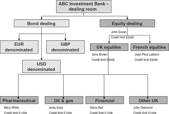
Note that the Equities Dealing Division has a total limit of GBP 500 000. There are two sections within the division, UK Equities and French Equities, both of which have individual limits of GBP 300 000. Obviously both sections cannot each use their entire limit, or else they would exceed the overall limit for the division. It is up to John Green, the head of the division, to arbitrate between his managers if they both wish to use their individual limits to the full. The same is true further down the tree; the four subsections of UK Equities have individual limits that exceed the limit for the section as a whole, and the section manager may need to arbitrate between her dealers.
Department and book limits are usually measured against the mark-to-market value of the portfolios. As well as an overall limit for each book, some firms may also issue additional limits based on criteria such as:
- A maximum limit for the value of total short positions
- A maximum limit for the value of total long positions
- Stop-loss limits for the individual instruments in the book
- Quality-based limits and restrictions – for example, for a bond portfolio there may be separate limits based on issuer credit ratings (refer to section 3.4.2).
- Concentration limits – for example, no individual security position can exceed x% of the total value of the book
- Sector limits – for example, the value of pharmaceutical stocks may not exceed x% of a particular limit, banking sector y%, etc.
Issuer limits
In Figure 24.1, it is possible that several trading books trade securities issued by the same issuer. For example, GlaxoSmithKline plc’s shares may be traded in the pharmaceuticals book, and its bonds may be traded in a number of different books depending on the issue currency. Many firms would apply an issuer limit to ensure that its total exposure to securities of all kinds issued by GlaxoSmithKline plc across all books was not greater than a pre-defined limit.
Counterparty and client limits
The same trading party may be a trading party for a number of different trade types in a number of different instruments. For example, Institutional Investor A may be a bond trading party, equity trading party, FX trading party, swap trading party, stock lending and repo counterparty, etc. The firm may wish to grant an absolute limit to the exposure that we are prepared to allow for Institutional Investor A, and additional limits for each business type. Counterparty limits are usually based on mark-to-market exposure less collateral placed, but not all firms will set up limits in the same way.
Country limits
Security issuers, trading parties and settlement agents must all be residents of a particular country, and some firms will wish to apply country limits to control and monitor the total exposure that the firm is willing to have to a particular country.
Parent limits and large exposures
An individual corporation in the financial sector could have (either directly or through subsidiaries) all of the following roles at the same time in relation to the firm that is managing limits:
- It is a securities issuer
- It is a trading party
- It is a settlement agent or payment bank.
Parent limits attempt to monitor the total exposure that the firm has to this type of complex organisation. European regulators require each firm to monitor its large exposures and to submit a quarterly return describing such exposures.
Software used to manage limits
There are a number of packaged applications designed to manage credit limits. The typical functions of such applications include:
- Limit type definition
- Limit basis definition
- Conglomerate ownership structure definition
- Real-time collection of trade data and current market prices from front-office systems to update limit utilisation records
- Ability to monitor trades pre-execution for potential limit breaches
- Real-time advice of limit breaches delivered to credit risk staff for them to take action
- Facilities for credit management to authorise temporary limit breaches
- Calculation of Value-at-Risk – refer to section 24.6.
If such an application is deployed, then many of the firm’s other systems will require real-time interfaces with that application.
24.6 AN INTRODUCTION TO VALUE-AT-RISK (VAR)
24.6.1 Overview of VaR
Value-at-Risk (VaR) is an estimate – not a precise measurement – of how the market value of an asset or of a portfolio of assets is likely to decrease over a certain time period (usually over one day or 10 days) under usual conditions. It was initially used by securities firms but was widely adopted by banks and corporates after 1994 when JP Morgan offered its RiskMetrics™ VaR measurement service over the internet in 1994. Firms that want to use the Basel Committee’s Advanced Measurement Approach (see “Basel II capital calculations for operational risk”, page 62, Chapter 8 to calculating their capital ratio are required to use the VaR technique.
A VaR statement is commonly expressed in the following way:
Our 20-day VaR is $4 000 000 with a 95% confidence level.
This means that the maximum that this firm would expect to lose over a 20-day period under “normal” market conditions is $4 000 000. However, they are only 95% confident of this estimate, which means that there is a 5% chance (one day out of the 20) that they could lose more than $4 000 000.
Normality in this context is a statistical concept and its importance varies according the VaR calculation methodology being used. Essentially VaR measures the volatility of a company’s assets, so the greater the volatility the higher the probability of loss.
24.6.2 The VaR calculation
The steps to setting up an application to perform a VaR calculation are as follows:
1. Determine the time horizons to use: Traders are often interested in calculating the amount they may lose in a single day. Basel II requires a 10-day horizon.
2. Select the degree of certainty required: Basel II requires 99%.
3. Create a probability distribution: There are several methods; the simplest depends upon collecting a history of price changes for the portfolio for the time horizon.
4. Gather the position data into a centralised database: Static data, position and price information for all the different instruments (which may be held and processed in a number of different business applications) must be gathered together in a single normalised database so that the calculation may be performed. Accurate static data is vital in this context; in particular quality of the instrument associations data (described in section 10.4.4) can have a considerable affect on the accuracy of the VaR prediction.
5. Make correlation assumptions: VaR requires that the user decides which exposures are allowed to offset each other and by how much. For example, are prices of physical commodities correlated to inflation rates; are crude oil prices correlated to natural gas prices, and to what degree?
6. Decide on the statistical model: There are three to choose from:
- Historical simulation method: This method assumes that asset returns in the future will have the same distribution as they had in the past (historical market data). It therefore uses actual historical data which means that rare events and crashes can be included in the results. It is the simplest and most transparent methodology.
- Correlation method: This method (also known as the variance–covariance method) assumes that risk factor returns are always (jointly) normally distributed and that the change in portfolio value is linearly dependent on all risk factor returns.
- Monte Carlo simulation method: Future asset returns are more or less randomly simulated using volatility and correlation estimates chosen by the risk manager. Monte Carlo simulation is often used to compute VaR for portfolios containing instruments such as options that have non-linear returns. Because the computational effort required is non-trivial, it is less often used for simpler portfolios.
24.6.3 Benefits, disadvantages and risks of using VaR
Benefits
- It provides a statistical probability of potential loss.
- It can make an assessment of the correlation between different assets.
- It translates all risks in a portfolio into a common standard – that of potential loss, allowing the quantification of firm-wide, cross-product exposures.
Disadvantages
- It does not account for liquidity risk.
- It is dependent on good historical price data. For this reason, it is most useful for financial instruments that have accurate and comprehensive records of market values for all instruments.
Risks
VaR has been developed as a means of predicting, or anticipating, future events. This is an imperfect process and the models can break down if the assumptions that they are based upon are violated. The risk of this happening is called model risk – the risk that models are applied to tasks for which they are inappropriate or are otherwise implemented incorrectly. For example, a firm is expanding operations into Asian emerging markets. It fails to modify its pricing models to reflect the lack of liquidity in these markets and underestimates the cost of hedging its positions.
An important aspect in the application of complex models is to understand the assumptions and test their accuracy as far as possible. This is achieved by performing back testing and stress testing.
Back testing is the practice of comparing the actual daily trading results to the predicted VaR figure. It is a test of reliability of the VaR methodology and ensures that the approach is of sufficient quality. It is usually performed on a daily basis by the risk management department and if the differences between reality and estimation are found to be unacceptable the VaR model must be revised. Back testing of course assumes that what happens in the past will happen in the future, and this assumption itself can create risks for the model.
Stress testing means testing the model against “extreme” market conditions. It can be thought of as capturing and considering particular risks that may, or may not, have been captured by the VaR calculation. Stress tests are not designed to generate worst case results. Stress testing is normally performed by the risk management department and is designed to improve the appreciation of market risk. The results can be fed back into the VaR model to improve it.
Stress testing scenarios can be constructed in either an ad hoc manner or a systematised manner. If the firm is concerned about the effect of an inverted yield curve or a breakdown in a specific correlation, an ad hoc scenario can be constructed specifically to assess that eventuality. Alternatively, firms may specify certain fixed scenarios (defined in terms of per cent changes in applicable risk factors) and then perform periodic stress testing with those scenarios. In this manner, a firm might present stress test results in its daily risk report.