CHAPTER 3

Survey of the Recent Literature: Recovery Risk

Sanjiv R. Das^a

1. INTRODUCTION

Default risk has two main components: the risk of default occurrence and the risk of recovery. The extant literature has focused widely on the former, and much too little attention has been given to recovery risk. This is changing, and many working papers on recovery risk have been written recently. This chapter reviews what we know about recoveries and highlights some of the new thinking in this area.

In discrete time, we may write the one-period spread as determined by the probability of default, which we denote as λ, and the loss rate given default (LGD) L = 1 – ϕ, where ϕ is the recovery rate. We restrict ourselves to an exposition in discrete time. Hence, we consider intervals ending at times {t₁,t₂,…,t_N}, where there are N periods and corresponding time points.

More generally, we may think of the credit spread for a given maturity as being a function of a vector of forward probabilities of default and recovery rates, as well as some firm-specific constants. We may write the spread (S) as

where λ = {λ_t1,λ_t2,…,λ_tn}. Likewise, we have recovery rates ϕ = {ϕ_tl, ϕ_t2,…,ϕ_tN}.

It is natural to expect that the relationship between spreads and default probabilities is a positive one, and that between spreads and recovery rates is negative. Hence,

This also suggests, but does not necessitate, a negative relationship between default rates and recovery rates, that is, Corr[λ,ϕ] <0. In some cases, this negative relationship is derived endogenously in the model (as in variants of the Merton (1974) model. In other cases, it is imposed exogenously, as in the paper by Bakshi et al. (2001).

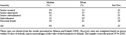
Before proceeding to models and empirical reality, it is worth summarizing the statistics available on recovery rates. These are all available in the work of Altman and Fanjul (2004) and other sources, many provided by Altman. The broad statistics on recovery seem to remain unchanged (mostly) year after year with uncanny stability. Consider Table 3.1, drawn from Altman and Fanjul. As can be seen, the overall median recovery rate is 40% and this has been very much the value for many years. Seniority determines most of the cross-sectional variation in recoveries. Recovery rates are highly variable within each category, for the standard deviations are relatively large in comparison to the means. This suggests that accurate estimates of recovery may be difficult to find.

Table 3.1 Recovery Rates for Publicly Traded Corporate Bonds

2. EMPIRICAL ATTRIBUTES

Apart from the raw statistics delineated above, there are many empirical findings that have recently been uncovered in the growing literature in this area. These are as follows:

1. There is a strong negative relationship between default rates and recovery rates on default. (Note that these are realized default rates, and are different from probabilities of default (PDs), which are forward-looking metrics.) Altman et al. (ABRS) (2005) find that this negative relationship is strong for various linear and nonlinear specifications. The R-squares are in the range of 65% and sometimes as high as 80%. The relationship is definitely nonlinear, as linear specifications result in much lower R²s of about 50%. In the ABRS paper, recovery rates appear to be negatively convex in the default rate; that is, as default rates increase, recovery rates fall, but tend to fall less with increasing default. There is a tendency toward an asymptotic lower bound for recovery rates; it suggests that the distributions of recovery rates are likely to be positively skewed. The negative correlation of default and recovery is natural ins models where both are driven by a common systematic factor.

   Estimates of the correlation vary widely. Hu and Perraudin (2002) find a negative correlation (≍–0.2) in their sample of US firms, whereas Carey and Gordy (2003) find only a very low and weak negative relationship in a 30-year sample of US defaults. Bakshi et al. (2001) report, in their study of lesser quality investment-grade debt, that a 4% increase in the probability of default results in a 1% decrease in recovery rates. Frye (2000) reports that in times of economic distress, recovery rates can drop by as much as 25%.

2. Recovery rates are very volatile. We can see this from the standard deviation of recovery rates in Table 3.1. A look at recovery rates over time, as presented in ABRS, shows that aggregate recovery rates went to a high of 62% in 1987, and reached a low of about 23% in 1990.

   This volatility, coupled with the negative correlation of default and recovery, implies that risk management measures such as credit value-at-risk (cVaR) that ignore these aspects of recovery empirics, must surely understate their risks. Simulation exercises in ABRS attempt to quantify the extent of this impact.

3. The supply of defaultable debt is also an important determinant of recovery rates. This thesis is developed and tested in the work of ABRS. They find that the total amount of high-yield bonds outstanding is inversely related to recovery rates in a statistically significant manner.
4. Seniority matters. From Table 3.1 we can see that this is clearly the case. Acharya et al. (2003) find this effect in a study of defaulted bonds over the last two decades, after controlling for many other causes.
5. Recovery rates depend on industry sector. This finding in Acharya et al. (2003) is robust to many controls. The authors imply that industry effects may be driving the influence of defaultable bond supply on recovery rates. An important implication of this work is that models of recovery rates should incorporate industry factors, and from the point of view of diversification, it makes sense to choose bonds across sectors, rather than within sectors. Sector recovery risk may also be hedged using sector-specific basket default contracts.
6. Regime effects impact recovery rates. As discussed, Frye (2000) shows that recoveries in economic downturns are substantially (≍25%) lower than what we see in normal times. In a recent paper, Hu (2004) provides an analysis of recovery rate distributions by seniority, rating class, and regime, and finds very different outcomes by regime. She fits regime-dependent beta distributions for recovery and finds starkly different shapes of the distributions. The implications for Monte Carlo simulation of recoveries is that regime-shifting is important to include in the model, especially for long-dated portfolios.
7. The beta distribution is proving to be the fitting model of choice. The probability density function for recovery rates is usually modeled as follows:

   

   where a and b are the parameters of the distribution, and β(a, b) is the beta function. The beta function is 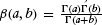. Hu (2004) shows that recovery rates over the last two decades fit this distribution well, and that there are two primary determinants of the fit: (1) the economic regime in which the recovery rate resides, and (2) the seniority of defaulted debt. She fits recovery rate data by setting the parameters of the beta distribution as functions of economic regimes and seniority. The differences across regime are striking, which implies that Monte Carlo simulation of recovery rates should also be based on regimes in order to capture scenarios in a comprehensive manner.

Overall, there is a clear relationship of recovery rates to defaults, industry factors, seniority, and economic regimes. All this evidence is also consistent with a high element of systematic risk driving default and recovery.

3. RECOVERY CONVENTIONS

Recovery rates are usually expressed in percentage terms, although under different metrics. Computing recovery depends on both the specification of the dollar amount recovered (the numerator) and the base against which comparison is made (the denominator).

While there are many ways in which the recovered amount may be assessed, two approaches seem to be common.

1. Recovery is measured as the value of bonds within the month after default. An observed price is sufficient to determine the value for this purpose.
2. Recovery is measured at the time of the final resale of the bonds, or the value in the final restructuring under a court agreement. This usually occurs long after the default date itself.

Which of these conventions is used often depends on the purpose for which recovery rates are required. In derivative pricing models, such as those required for valuing default swaps, the former measure is the more appropriate one. However, in empirical analyses, in which the end-game value of a Chapter 7 or 11 out come is being assessed, quite clearly we are interested in the latter specification.

The second part of the recovery rate specification lies in expressing the recovered amount as a percentage of a baseline value. We encounter three popular conventions here:

1. Recovery of par (RP): Here the recovered amount is expressed as a fraction of the par value of the security.
2. Recovery of Treasury (RT): Recovery is a fraction of the value of a similar risk-free bond.
3. Recovery of market value (RMV), where the recovery amount is taken as a fraction of the price of the security if it had not defaulted. This is sometimes similar to expressing recovery as a percentage of the price of the bond just prior to default, provided default comes as a complete surprise.

In a recent model, Bakshi et al. (2001) fit models to BBB bond data and assessed which of these conventions resulted in a better empirical fit. They found that the best approach was the Recovery of Treasury (RT) assumption. They also discussed how to take their fitted model and move between the physical and risk-neutral measures for recovery rates. We will consider this later.

4. RECOVERY IN STRUCTURAL MODELS

The line of structural models beginning with Merton (1974) are based on modeling the underlying firm value, and then determining the values of risk-neutral default and recovery as functions of firm value. Thus, both default and recovery are endogenous in this class of models. We undertake a simple exposition here.

Let the initial value of the firm be V₀. At the maturity (T) of the debt in the firm, the value of the firm V_T must be below the face value of debt D for the firm to be in default. It is easy to see that this directly provides the recovery rate, that is,

The expected recovery is simply

Note that

The previous two equations may be used to write the equation for recovery as follows:

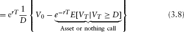
This is a very simple expression for recovery rates in the Merton model. It is easily checked that this implies an endogenous negative correlation between default and recovery. This analytic equation may also be easily extended to models where a default barrier is used.

There are structural models in which the recovery rate is exogenously imposed and is not derived within the model. This is the approach taken in the model developed by CreditMetrics (Gupton et al. 1997). In fairness, this idea was originally employed in a model by Nielsen et al. (1993). This model posits the form originally used in Black and Cox (1976), where default occurs not just at maturity, as in the Merton model, but also at times prior to maturity, if the value of the firm accesses a default boundary. The innovation adopted in the CreditMetrics model is to make the default barrier stochastic, which plays the important role of making spreads larger and more volatile.

5. RECOVERY IN REDUCED-FORM MODELS

In reduced-form models, the recovery rate is not endogenously available as in structural models. It needs to be exogenously supplied. Hence, it is an additional input to the modeling process. As noted in the beginning of this chapter, spreads are a function of the probability of default and the loss rate (1 – ϕ). Hence, it is not possible to disentangle recovery rates from spreads without making an assumption about the probability of default, or vice versa. This has been pointed out in many articles (see, e.g., Duffie and Singleton, 1999) and various suggestions have been made to work around this problem.

A recent paper by Chan-Lau (2003) develops a way of extracting recovery rates from the default swap markets. These markets are fast becoming the calibration anvil for reduced-form models. The innovation in this approach lies in exploiting the relationship of default probabilities and recovery rates to spreads in a manner that achieves bounds on recovery rates, rather than point estimates. We briefly review this approach here.

Consider a discrete-time model with N periods, indexed by i = 1,2,…, N. Hence, we have times 0, t₁,…, t_i,…, t_N. For simplicity, we let the intervals h for each period be constant, that is, h = t_N/N.

The forward rate between t_i–1 and t_i is denoted as f(t_i), which is the one-period forward rate ending at time t_i. Within each period, default probabilities are assumed to remain constant, and are denoted as λ_i ≡ λ(t_i). Default probabilities are stated in annualized form. Therefore, the survival probability from time 0 to time t_i is

Suppose the N-period default swap premium is c_N% per year. Then, the premium paid per period on a notional of $100 is equal to C_N × h. We may express the expected discounted value of the premium payment in period i as follows:

The total expected premium on the entire default swap is

Assume that the recovery rate is constant and is, as before, denoted by ϕ. Then, the expected discounted payoff from the default payment on the swap in period i is

The total expected discounted payoffs on default are

In a fair-value default swap we must have the premiums equalling the payoffs in discounted expectation (under the martingale measure):

Given a set of swap premiums, we may bootstrap the values of s(t_i) for all maturities. We begin with N = t₁, and assuming a fixed ϕ, we solve for s(t₁), given a known premium c₁. Next, we use premium c₂, and the previously computed s(t₁) to obtain s(t₂). And so on up the maturity curve until we have all the survival probabilities.

Chan-Lau (2003) suggests that we may think of the survival probabilities as functions of the chosen recovery rate ϕ. Setting the recovery rate too high would imply negative survival probabilities in order to be consistent with spreads. Hence, there must be a “maximal” recovery rate that admits a set of acceptable survival probabilities across all maturities.

This maximal recovery rate, labeled , is extracted in Chan-Lau's working paper for various emerging market debts, cross-sectionally, on a daily basis. The time series of maximal recovery rates is then compared across countries to determine the features of cross-border correlations. Interestingly, he also finds that drops sharply in advance of Argentina's recent default crisis.

6. MEASURE TRANSFORMATIONS

In both of the preceding sections, recovery rates were extracted from models via calibration to the prices of traded securities. Therefore, the recovery rates are obtained under the pricing (risk-neutral) probability measure. For the purpose of risk management, these need to be converted into recovery rates under the statistical (physical) measure. This matter is ably addressed in the paper by Bakshi et al. (2001). We present their model (in simplified form) here.

In the world under the physical measure, we define the probability of default to be , a constant. The recovery rate is random and will be high or low as follows:

Naturally, conversion to and from the risk-neutral and physical measures requires the risk premium for recovery risk. This premium depends on the specific utility function chosen. We work here without necessarily specifying the form of the utility function.

Assume a representative investor with initial wealth W₀, which includes a defaultable security that promises to pay F at maturity. Utility is designated to be a function of terminal wealth (W) in this, a one-period model, that is, U(W).

The investor can buy a default protection contract on the defaultable security now at cost C₀. In the event of default, the investor's payoff from the protection contract will be C_H or C_L, with C_H > C_L, dependent on the recovery rate realized with the probabilities above. Interest rates are zero in the model. We set the number of units of the hedge contract to be x.

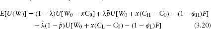
The outcomes of the model are threefold: (1) No default occurs, (2) Default occurs and recovery is ϕ_H, or (3) Default occurs and recovery is ϕ_L. The three respective terminal wealth values are as follows:

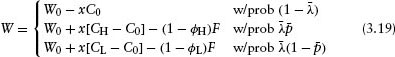
We may write the expected utility of these outcomes as

It is easy now to solve for x, by differentiating the expected utility with respect to x and setting the result equal to zero:

Substituting x in gives , that is, the optimal utility function.

This preceding analysis was carried out under the physical measure. Were the same optimization done with a risk-neutral investor, the expected utility would be

where E(·), λ, and p are written differently compared to and as before, to signify that the analysis is under the risk-neutral measure. Also, note that there is no purchase of a default protection contract, as the investor is neutral to credit risk.

Equating , we get a single equation mapping to {λ, p}. In the special case that g106 ϕ_H = ϕ_L = 1, there is no recovery risk. In this case we may solve for λ in terms of . Once we have this, then we may use the equation above to solve for p. The risk premium for recovery would be related to the Radon-Nikodym derivative (/p).

Bakshi et al. (2001) calibrate a full-blown version of this model to BBB bonds, and in out-of-sample forecasts, find the best empirical support for the RT assumption. In addition, by offering a way in which physical measure recovery assumptions may be taken and translated into risk-neutral ones for pricing, there is much practical value in this model.

In a follow-up paper to the abovementioned work, Zhang (2003) develops a multifactor model of default swap pricing, and examines the implied recovery forecasts from the model of Argentina's sovereign debt default. The model separates recovery rates from default probabilities. In the period much before default, the model calibrates very well, but performs less well closer to default, no doubt on account of additional factors affecting the market not picked up in the parsimonious model that was used. Short maturity contracts are particularly hard to price.

This model is a tour de force. It provides closed-form solutions, and as expected, finds that risk-neutral default probabilities are higher than those under the statistical measure. The default-risk premium is very volatile over the sample. The model's factors align well with the slope of the US term structure, the level of long-term rates, and the J. P. Morgan emerging market bond index (EMBI).

7. SUMMARY AND SPECULATION

Recovery models are truly proving that creative theory helps makes good sense of possibly weak data. We know a lot now about the determinants of recovery rates and their relationship to default probabilities. Improvements in our models are resulting in tighter bounds on the range of recovery rates. These models are tractable and simple to calibrate.

Models help in transforming general uncertainty into quantifiable risk. It is at the cusp of this metamorphosis that new markets are born. We appear to be close to seeing rapid growth in markets for recovery risk.

REFERENCES

Acharya, V., Bharath, S. and Srinivasan, A. (2003). “Understanding the Recovery Rates on Defaulted Securities.” Working Paper, London Business School.

Altman, E. and Fanjul, G. (2004). “Defaults and Returns in the High-Yield Bond Market: Analysis through 2003.” Working Paper, NYU Salomon Center.

Altman, E., Resti, A. and Sironi, A. (2003). “Default Recovery rates in Credit Risk Modeling: A Review of the Literature and Empirical Evidence.” Working Paper, New York University.

Altman, E., Brady, B., Resti, A. and Sironi, A. (2005).“The Link between Default and Recovery Rates: Theory, Empirical Evidence and Implications.” Journal of Business 79(1), forthcoming.

Bakshi, G., Madan, D. and Zhang, F. (2001). “Recovery in Default Risk Modeling.” Working Paper, University of Maryland.

Black, F. and Cox, J. (1976). “Valuing Corporate Securities: Some Effects of Bond Indenture Provisions.” Journal of Finance 31(2), 351–367.

Carey, M. and Gordy, M. (2003). “Systematic Risk in Recoveries on Defaulted Debt.” Working Paper, Federal Reserve Board, Washington.

Chan-Lau, J. A. (2003). “Anticipating Credit Events Using Credit Default Swaps, with an Application to Sovereign Debt Crisis.” IMF Working Paper.

Duffie, D. J. and Singleton, K. J. (1999). “Modeling Term Structures of Defaultable Bonds.” Review of Financial Studies 12, 687–720.

Frye, J. (2000). “Collateral Damage Detected.” Working Paper, Federal Reserve Bank of Chicago, Emerging Issues Series, October, 1–14.

Gupton, G., Finger, C. and Bhatia, M. (1997). “CreditMetrics Technical Document.”J. P. Morgan & Co., New York.

Hu, W. (2004). “Applying MLE Analysis to Recovery Rate Modeling of U.S. Corporate Bonds.” MS Thesis, UC Berkeley, Haas School of Business.

Hu, Y.-T. and Perraudin, W. (2002). “The Dependence of Recovery Rates and Default.” Working Paper, Birkbeck College.

Jarrow, R. A. (2001). “Default Parameter Estimation Using Market Prices.” Financial Analysts Journal 57(5), 75–92.

Jokivuolle, E. and Peura, S. (2003). “Incorporating Collateral Value Uncertainty in Loss-Given-Default Estimates and Loan-to-Value Ratios.” European Financial Management 9(3), 299–314.

Merton, R. C. (1974). “On the Pricing of Corporate Debt: The Risk Structure of Interest Rates.” The Journal of Finance 29, 449–470.

Nielsen, L., Saa-Requejo, J. and Santa-Clara, P. (1993). “Default Risk and Interest Rate Risk: The Term Structure of Credit Spreads.” Working Paper, INSEAD & UCLA.

Zhang, F. X. (2003). “What Did the Credit Market Expect of Argentina Default? Evidence from Default Swap Data.” Working Paper, Federal Reserve Board.

Zhou, C. (2001). “The Term Structure of Credit Spreads with Jump Risk.” The Journal of Banking and Finance 25, 2015–2040.

Keywords: Recovery; loss rate; risk-neutral; measure