CHAPTER 9

Correlated Default Processes: A Criterion-Based Copula Approach

Sanjiv R. Das^a,* and Gary Geng^b

1. INTRODUCTION

Default risk at the level of an individual security has been extensively modeled using both structural and reduced-form models.¹ This chapter examines default risk at the portfolio level. Default dependences among issuers in a large portfolio play an important role in the quantification of a portfolio's credit risk exposure for many reasons. Growing linkages in the financial markets have led to a greater degree of joint default. While the actual portfolio loss due to the default of an individual obligor may be small unless the risk exposure is extremely large, the effects of simultaneous defaults of several issuers in a well-diversified portfolio could be catastrophic. In order to efficiently manage and hedge the risk exposure to joint defaults, a model for default dependencies is called for. Further, innovations in the credit market have been growing at an unprecedented pace in recent years and will likely persist in the near future. Many newly developed financial securities, such as collateralized debt obligations (CDOs), have payoffs depending on the joint default behavior of the underlying securities.² In order to accurately measure and price the risk exposure of these securities, an understanding and accurate measurement of the default dependencies among the underlying securities is essential.³ Accurate specification of default correlations is required in the pricing of basket default contracts. Correlation specifications are critical, as the baskets are not large enough to ensure diversification. Finally, the Basle Committee on Banking Supervision has identified poor portfolio risk management as an important source of risk for banking institutions. As a result, banks and other financial institutions have been required to measure their overall risk exposures on a routine basis. Default correlation is again an important ingredient to integrate multiple credit risk exposures.

In this chapter, we use Moody's default database to develop a parsimonious numerical method of modeling and simulating correlated default processes for hundreds of issuers. Using copula functions, we capture the stylized facts of individual default probabilities as well as the dynamics of default correlations documented in Das et al. (2001a) (DFGK, 2001a). Our methodology is criterion-based; that is, it uses a metric that compares alternative specifications of the joint default distribution using three criteria: (1) the level of default risk, (2) the asymmetry in default correlations, and (3) the tail dependence of joint defaults. We elaborate on these in what follows.

The base unit of joint credit risk is the probability of default (PD) of each issuer. Many popular approaches exist for computing PDs in the market place, developed by firms such as KMV Corporation, Moody's Risk Management Systems (MRMS), Risk Metrics, and so forth. In the spirit of reduced-form models, the default probability of issuer i at time t is usually expressed as a stochastic hazard rate, denoted as λ_i(t), i = 1,…, N. This chapter empirically examines the joint stochastic process for hazard rates, λ_i(t), for N issuers.

We fit a joint dynamic system to the intensities (or hazard rates) of roughly 600 issuers classified into six rating categories. Our approach involves capturing the correlation of PD levels across the six rating classes, and the correlation of firms' PDs within each rating class. We find (1) the appropriate copula function (for the joint distribution), (2) the stochastic process for rating-level default probabilities, and (3) the best set of marginal distributions for individual issuer default probabilities.

At the rating level, we choose from two classes of stochastic processes for the average hazard rate of the class: a jump-diffusion model and a regime-switching one. At the issuer level, we choose from three distributional assumptions: a normal distribution, a Student's t distribution, and a skewed double exponential distribution. We compare these distributions for each issuer using four goodness-of-fit criteria. At the copula level, we choose from four types: normal, Student's t, Gumbel, and Clayton. These inject varying amounts of correlation emanating from the joint occurrence of extreme observations.⁴

The various combinations of choices at the rating, issuer, and copula levels result in 56 different systems of joint variation. To compare across these, we develop a metric to determine how well different multivariate distributions fit the observed covariation in PDs. The metric accounts for the level of correlations, asymmetry of correlations, and the tail dependence in the data.

An important issue we look at here is tail dependence. Tail dependence is the feature of the joint distribution that determines how much of the correlation between default intensity processes comes from extreme observations and how much from central observations. For example, imagine two different bivariate distributions with the same standard normal marginal distributions. One distribution has a normal copula and the other a Student's t copula with a low degree of freedom. The former has lower tail dependence than the latter, which generates more joint tail observations. Hence, from a risk point of view, given the marginal distributions, the second joint distribution would be riskier for a large class of risk-averse investors. Our study sheds light on the tail dependence for default risk in a representative data set of US firms.

Our study of joint default risk for US corporates using copula techniques finds that the best choice of copula depends on the marginal distributions and stochastic processes for rating level PDs. The Student's t copula is best when the jump-diffusion model is chosen for the default intensity of each rating class. However, the normal or Clayton copula is more appropriate when the regime-switching model is chosen for rating level intensities. In general, our metric prefers a regime-switching model to a jump-diffusion one (for rating-level intensities), irrespective of the choice of marginal distributions. A perusal of the time-series plot of the data (see Figure 9.1) provides intuitive support for this result. While the regime-switching model for rating-level intensities is best, no clear winner emerges among the competing copulas. The interdependence between copula and marginal distributions justifies our wide-ranging search of over 56 different specifications.

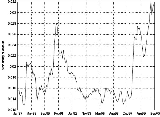
FIGURE 9.1 Time series of average PDs. This figure depicts the average level of default probabilities in the data set. The data show the presence of two regimes, one in which PDs were high, as in the early and later periods of the data, and the other in which PDs were much lower, less than half of those seen in the high-PD regime. Complementary analysis of correlated default by subperiod on the same data set in the same time frame is presented in DFGK (2001a).

We also assess the impact of different copulas on risk-management measures. An examination of the tail loss distributions shows that substantial differences are possible among the 56 econometric specifications. Arbitrarily assigning high kurtosis distributions to a copula with tail dependence may result in the unnecessary overstatement of joint default risk. Since different copulas inject varied levels of tail dependence, the metric developed in this chapter allows fine-tuning of the specification, which enhances the accuracy of credit VaR calculations.

The rest of the chapter proceeds as follows. In Section 2 we briefly describe the data on intensities. Section 3 provides the finance reader with a brief introduction to copulas, and Section 4 contains the estimation procedure and results. Section 5 presents the simulation model and the metric used to compare different copulas. Section 6 concludes.

2. DESCRIPTION OF THE DATA

Our data set comprises issuers tracked by Moody's from 1987 to 2000. For each issuer, we have PDs based on the econometric models for every month the issuer was tracked by Moody's. Moody's calibrates the PDs to match the level of realized defaults in the economy. Issuers are divided into seven rating classes. Rating classes 1 through 6 reflect progressively declining credit quality. Many more issuers fall into rating class 7, which comprises unrated issuers; the PDs within this class range from high to low, resulting in an average PD that is close to the median PD of all of the other rating classes. We do not consider PDs from rating class 7. We considered firms that had a continuous sample over the period. We obtained data on a total of 620 issuers classified into six rating classes. Our data set does not contain data from firms in the financial sector. These 1-year default probabilities were converted into intensities using an assumption of constant hazard rates, that is, λ_it = –ln(1 – PD_it). Table 9.1 provides a summary of Moody's rating categories for bonds.

The time series of average default probabilities is presented in Figure 9.1. Table 9.2 presents the descriptive statistics of our data from rating classes 1 through 6. The mean increases from rating class 1 to 6, as does the standard deviation. PD changes tend to be higher for lower-grade debt. Table 9.3 presents the dependence between rating classes measured by Kendall's τ statistic, a means of determining the dependence between any two time series. Higher-grade debt evidences more rank correlation in PDs than low-grade debt. This highlights the fact that high-grade debt is more systematically related, and low-grade debt experiences greater idiosyncratic risk.

Table 9.1 Moody's Rating Categories for Bonds in Descending Order of Credit Quality

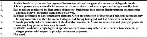
Table 9.2 Summary of Time Series of Average PDs for Each Rating Class. Each time series represents a diversified portfolio of issuers within each rating class^a

Table 9.3 Kendall's τ for Probabilities of Default for Rating Classes^a

3. COPULAS AND FEATURES OF THE DATA

3.1 Definition

We are interested in modeling an n-variate distribution. A random draw from this distribution comprises a vector X ∈ Rⁿ = {X₁,…, X_n}. Each of the n variates has its own marginal distribution, F_i(X_i), i = 1,…, n. The joint distribution is denoted as F(X). The copula associated with F(x) is a multivariate distribution function defined on the unit cube [0, 1]ⁿ. When all the marginals, F_i (X_i), i = 1,…, n, are continuous, the associated copula is unique and can be written as

Every joint distribution may be written as a copula. This is Sklar's Theorem (Sklar, 1959, 1973). For an extensive discussion of copulas, see Nelsen (1999).⁵

Copulas allow the modeling of the marginal distributions separately from their dependence structure. This greatly simplifies the estimation problem of a joint stochastic process for a portfolio with many issuers. Instead of estimating all of the distributional parameters simultaneously, we can estimate the marginal distributions separately from the joint distribution. Given the estimated marginal distribution for each issuer, we then use appropriate copulas to construct the joint distribution with a desired correlation structure. The best copula is determined by examining the statistical fit of different copulas to the data.⁶

Copula techniques lend themselves to two types of credit risk analysis. First, given a copula, we can choose different marginal distributions for each individual issuer. By changing the types of marginal distributions and their parameters, we can examine how individual default affects the joint default behavior of many issuers in a credit portfolio. Second, given marginal distributions, we can vary the correlation structures by choosing different copulas, or the same copula with different parameter values.

3.2 Copulas Used in the Chapter

In this chapter, in order to capture the observed properties of the joint default process, we consider the following four types of copulas:

Normal copula: The normal copula of the n-variate normal (Gaussian) distribution with correlation matrix ρ, is defined as

where Φ(u) is the normal cumulative distribution function (CDF), and F^–1(u) is the inverse of the CDF.

Student's t copula: Let T_ρ,v be the standardized multivariate Student's t distribution with v degrees of freedom and correlation matrix ρ. The multivariate Student's t copula is then defined as follow:

where t_v^–1 is the inverse of the cumulative distribution function of a univariate Student's t distribution with v degree of freedom.

Gumbel copula: This copula was first introduced by Gumbel (1960) and can be expressed as follows:

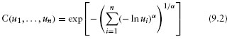
where α is the parameter determining the tail dependence of the distribution.

Clayton copula: This copula, introduced in Clayton (1978), is as follows:

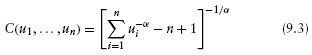
Again, α > 1 is a tail dependence parameter.

The procedure for simulating an n-dimensional random vector from the above copulas can be found in Wang (2000), Bouye et al. (2000), and Embrechts et al. (2001).

3.3 Tail Dependence

An important feature of the use of copulas is that it permits varying degrees of tail dependence. Tail dependence refers to the extent to which the dependence (or correlation) between random variables arises from extreme observations.

Suppose (X₁, X₂) is a continuous random vector with marginal distributions F₁ and F₂. The coefficient of upper tail dependence is:

If λ_U > 0, then upper tail dependence exists. Intuitively, upper tail dependence is present when there is a positive probability of positive extreme observations occurring jointly.⁷

For example, the Gumbel copula has upper tail dependence with λ_U = 2 – 2^1/α. The Clayton copula has lower tail dependence with λ_L = 2^–1/α. The Student's t has equal upper and lower tail dependence with λ_U =

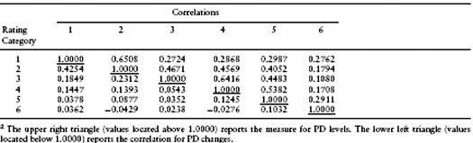
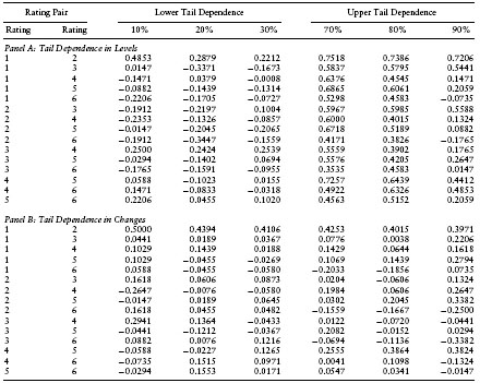
Table 9.4 provides a snapshot of the tail dependence between rating classes. The results in the table present the correlations between rating pairs over observations in the tails of the bivariate distribution. Results are provided both in levels and in changes. There is strong positive correlation in the upper tail, evidencing upper tail dependence. Correlations in the lower tail are often low and negative, and hence there is not much evidence of lower tail dependence.

Table 9.4 Correlations Between Hazard Rates among Rating Classes as Measures of Tail Dependence among observations in the bottom 10th, 20th, and 30th percentiles, and the correlations in the top 10th, 20th, and 30th percentiles; that is, the cutoffs are the 70th, 80th, and 90th percentiles. The values in the table are the correlations when observations from the second rating in the pair of rating classes lie in the designated portion of the tail of the distribution.

3.4 Empirical Features of Dependence in the Joint Distribution

In order to compare the statistical fitting of joint distributions associated with different copulas, we develop a metric that captures three features of the dependence relationship in the joint distribution:

• Correlation levels: We wish to ensure that our copula permits the empirically observed correlation levels in conjunction with the other moments. This depends on the copula and the attributes of the data
• Correlation asymmetry: Hazard rate correlations are level-dependent, and are higher when PD levels are high—correlations increase when PD levels jump up, and decrease when PDs jump down.
• Tail dependence: It is important that we capture the correct degree of tail dependence in the data, that is, the extent to which extreme values drive correlations.

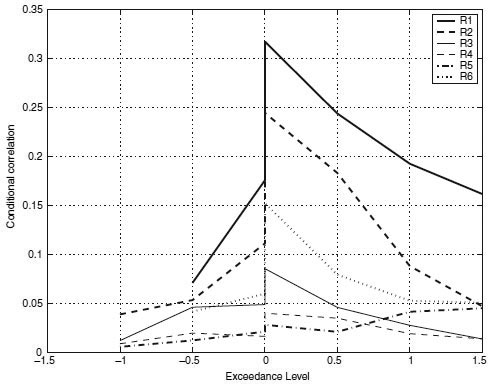
FIGURE 9.2 Asymmetric exceedance correlations of PD's for the different rating classes. The plots are consistent with the presence of asymmetric correlation. Complementary analysis of correlated default by sub period in this same time frame is presented in DFGK (2001a) where different analyses are conducted on the same data set.

Following Ang and Chen (2002) and Longin and Solnik (2001), we present the correlations for different rating classes in a correlation diagram (see Figure 9.2). This plot is created as follows. We compute the total hazard rate (THR) across issuers (indexed by i) at each point in time (t), that is, THR_t = Σ^N_i=1 λ_i(t), ∀t. We normalize the THR by subtracting the mean from each observation and dividing by the standard deviation. We then segment our data set based on exceedance levels (ξ) determined by the normalized THR. Our exceedance levels are drawn from the set ξ = {−1.5, −1.0, −0.5, 0, 0, 0.5, 1.0, 1.5}. (Note that zero appears twice because we account for both left and right exceedance.) Ang and Chen (2002) developed a version of this for bivariate processes. Our procedure here is a modification for the multivariate case. For example, the exceedance correlation at level –ξ is determined by extracting the time series of PDs for which the normalized THR is less than –ξ, and computing the correlation matrix therefrom. We then find the average value of all entries in this correlation matrix to obtain a summary number for the correlation in the rating class at the given exceedance level. These are plotted in Figure 9.2. There is one line for each rating class. The line extends to both the left and the right sides of the plot. To summarize, the exceedance graph shows (for each rating category) the correlation of default probabilities when the overall level of default risk exceeds different thresholds. As threshold levels become very small or very large, correlations decline, and the rate at which they decline indicates how much tail dependence there is.

The three features of the dependence relationship are evident from the graph. First, the height of the exceedance line indicates the level of correlation, and we can see that high-grade debt has greater correlation than lower-grade debt (see Xiao (2003) for a similar result with credit spreads). Second, there is clear evidence of correlation asymmetry, as correlation levels are much higher on the right side of the graph; that is, when hazard rate changes are positive. Third, the amount of tail dependence is inferred from the slope of the correlation line as the exceedance level increases. The flatter the line, the greater the amount of tail dependence. As absolute exceedance levels increase, we can see that correlation levels drop. However, they fall less slowly if there is greater tail dependence. We can see that lower-grade debt appears to have more tail dependence than higher-grade debt.

Overall, the exceedance plot shows that bonds within high-quality ratings have greater default correlation than bonds within low-quality ratings. However, tail dependence is higher for lower-rated bonds. Both results are intuitive—high-grade debt tends to be issued by large firms that experience greater amounts of systematic risk, and low-grade firms evidence more idiosyncratic risk; however, when economy-wide default risk escalates, low-grade bonds are more likely to experience contagion, leading to greater tail dependence.

4. DETERMINING THE JOINT DEFAULT PROCESS

4.1 Overall Method

Our data comprise firms categorized into six rating classes. We average across firms within rating class to obtain a time series of the average intensity (λ_k) for each rating class k. We assume that the stochastic processes for the six average λ_ks are drawn from a joint distribution characterized by a copula, which establishes the joint dependence between rating classes. The correlation matrix for the mean intensities is calculated directly from the data. The copula is set to one of four possible choices: normal, Student's t, Gumbel, or Clayton. The form of the stochastic process for each average hazard rate is taken to be either a jump-diffusion or a regime-switching one. This setup provides for the correlation between rating classes.

Next, the correlations within a rating class are obtained from the linkage of all firms in a rating class to the mean PD process of the rating category. We model individual firm PDs as following a non-negative stochastic process with reversion to the stochastic mean of each rating.

To conduct a Monte Carlo simulation of the system, we propagate the average rating PDs using either a jump-diffusion or a regime-switching model, with correlations across ratings given by a copula. Then we propogate the individual issuer intensities using stochastic processes that oscillate around the rating means. The entire system consists of a choice of (1) stochastic process for average intensities (jump-diffusion versus regime-switching), (2) copula (normal, Student's t, Gumbel, Clayton), and (3) marginal distribution for issuer-level stochastic process for intensities (one of seven different options). All told, therefore, we have 56 alternate correlated default system structures to choose from.

4.2 The Estimation Phase

Estimation is undertaken in a two-stage manner: (1) the estimation of the stochastic process for the mean intensity of each rating class, and (2) the estimation of the best candidate distribution for the stochastic process of each individual issuer's intensity. We choose two processes for step (1). Both choices are made to inject excess kurtosis into the intensity distribution. First, we use a normal jump model. Second, we use a regime-switching model. Each is described in turn in the next two subsections.

4.2.1 Estimation of the Mean of Each Rating Class Using a Jump Model

For our six rating classes (indexed by k) and all issuers (indexed by j), we compute intensities from the probabilities of default (P_kj, j = 1,…, N_k, k = 1,…, 6) in our data set. The intensities are computed as λ_kj = – ln(1 – P_kj) ≥ 0. We denote M as the total number of rating classes and N_k as the total number of issuers within the rating class for which data are available.

Let λ_k(t) be the average intensity across issuers within rating class k. Therefore, λ_k(t) = 1/N_k Σ_j=1^Nk λ_kj(t),∀t. We assume that λ_k(t) follows the stochastic process:

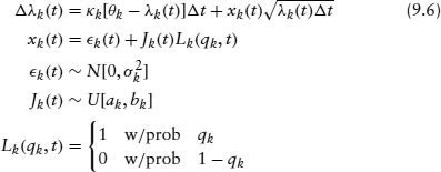
We assume that the jump size J_k follows a uniform distribution over [a_k, b_k].⁸ This regression accommodates a mean-reverting version of the stochastic process, and κ_k calibrates the persistence of the process. This process is estimated for each rating class k, and the parameters are used for subsequent simulation. Copulas are used to obtain the joint distribution of correlated default. The correlation matrix used in the copula comes from the residuals x_k(t) computed in the regression above.

We use maximum likelihood estimation (MLE) to obtain the parameters of this process. Since there is a mixture of a normal and a jump component, we can decompose the unconditional density function for the residual term x_k(t) into the following:

The latter density, f[x_k(t) | L_k = 0], is conditionally normal. The marginal distribution of x_k(t) conditional on L_k = 1 can be derived as follows:

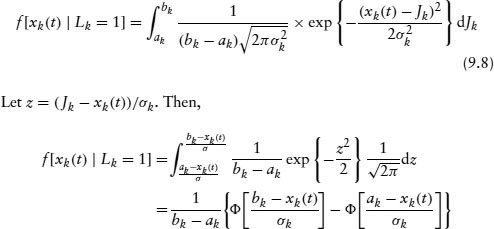
Table 9.5 Results of Stochastic Process for Estimating Mean of the Intensities of Each Rating Class. Numbers below the estimates are the t-statistics from the estimation, which is undertaken by maximum likelihood

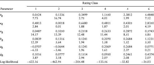
In the case when a_k = b_k, the process has a constant jump size with probability 1, and the marginal distribution of x_k(t) degenerates to a normal distribution with mean a_k and standard deviation σ_k. This can be seen by letting b_k = a_k + c. We then have

where φ(·) and Φ(·) are the standard normal density and distribution functions, respectively. Because jumps are permitted to be of any sign, we may expect that b_k ≥ 0 and a_k ≤ 0. Also, if |b_k| > |a_k|, it implies a greater probability of positive jumps. When a_k is close to b_k, or when they have the same sign, the process has a constant or a one-direction jump, respectively.

The estimation results are presented in Table 9.5. The mean of the intensity process (θ_k) increases with rating class k, as expected. The variance (σ_k) also increases with declining credit quality. Generally speaking, the probability of a jump (q_k) in the hazard rate is higher for lower quality issuers. We can see that rating classes 3 to 5 have a constant jump and rating 6 has only a positive jump. While the mean jump for all rating classes appears to be close to zero, that for the poorest rating class is much higher than zero. Hazard rates jump drastically when a firm approaches default.

After obtaining the parameters, we compute residuals for each rating class. The residuals include randomness from both the normal and the jump terms. The covariance matrix of these residuals is stored for later use in Monte Carlo simulations.

4.2.2 Estimating the Mean Processes in a Regime-Switching Environment

From Figure 9.1, we note that there are periods in which PDs are low, interjected by smaller sporadic regimes of spikes in the hazard rates. A natural approach to capture this behavior is to use a regime-switching model.⁹

In order to determine regimes, we first compute the average intensity (hazard rate, approximately), = Σ_i=1^N λ_i, across all issuers in our database. Within each regime the intensity is assumed to follow a square-root volatility model represented in discrete time as follows:

The two regimes are indexed by r, which is either HI or LO. κ_r is the rate of mean reversion. The mean value within the regime is θ_r, and σ_r is the volatility parameter.

The probability of switching between regimes comes from a logit model based on a transition matrix:

where p_r = exp(α_r)/(1 + exp(α_r)), r ∈ {LO, HI}. Estimation is undertaken using maximum likelihood. We fix the values of θ_r based on the historical PDs, with a high–low regime cutoff of 2%. θ_LO was found to be 1.68% and θ_HI to be 2.40%.¹⁰ We then estimate the rest of the parameters in the above model. The estimation results are presented in Table 9.6. In the high-PD regime, the higher level of hazard rates is matched by a higher level of volatility.

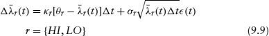
Our next step is to use the determined regimes to estimate the parameters of the mean process for each rating class, that is, λ_k, k = 1, …, 6. We fit regime-shifting models to each of the rating classes, using a stochastic process similar to that in equation 9.9:

Table 9.6 Estimation Results of Regime-Switching Model for Regimes Estimated on Average Intensity Process ( = Σ^Ni=1 λ_i) across All Issuers in Data Set. We designated periods in which ≤ 2% as the “low-PD” regime, and periods in which < 2% as the “high-PD” regime. The two regimes are indexed by r, which is either HI or LO. κ_r is the rate of mean reversion. The mean value within the regime is θ_r, and σ_r is the volatility parameter. The probability of switching between regimes comes from a logit model based on a transition matrix: where p_r = exp(α_r)/(1 + exp(α_r)), r ∈ {LO, HI}. Estimation is undertaken using maximum likelihood.

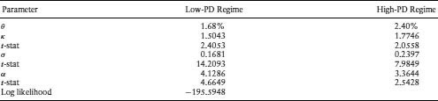
Table 9.7 Estimation Parameters of Regime-Switching Model for Mean of Each Rating Class: This table presents parameters for the regime-switching model applied to the mean process for each rating class, i.e., _k, k = 1, …, 6.

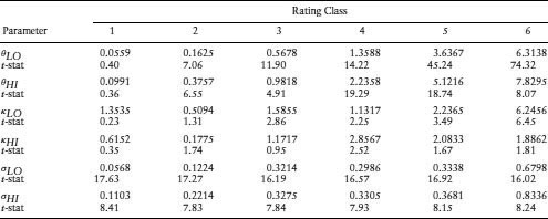
The results of the estimation are presented in Table 9.7. The parameters are as expected. The mean of the processes is higher in the high regime, as is the volatility. We now proceed to look at the choice of individual issuer marginal distributions.

4.2.3 Estimation of the Stochastic Process for Each Individual Issuer

Assume that the intensity for each individual issuer follows a square-root process:

We normalize the residuals by dividing both sides by We then use ordinary least squares to estimate parameters, which are stored for use in simulations. The resulting residuals are used to form the covariance matrix for each class.

The long-term mean is defined as the sum of a constant number θ_kj and the group mean λ_k(t) multiplied by a constant, γ_kj. This indexes the mean hazard rate for each issuer to the current value of the mean for the rating class. Consequently, there are four parameters for each regression, κ_kj, θ_kj, γ_kj, and σ_kj. Note that κ_kj should be positive; θ_kj and γ_kj can be positive or negative as long as they are not both negative at the same time. None of the issuers has negative θ_kj and γ_kj at the same time, although 20 issuers have negative κ_kj. We, therefore, deleted the 20 issuers with negative κ from our dataset for further analysis.¹¹

4.2.4 Estimation of the Marginal Distributions

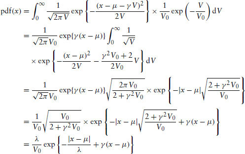
We fit the residuals from the previous section to the normal, Student's t, and skewed double exponential distributions. We use prepackaged functions in Matlab for maximum-likelihood estimation (MLE) for the normal and Student's t distributions. The likelihood function for the skewed double exponential distribution is as follows. Assume that the residual ε_kj has a normal distribution with mean γV and variance V. Further, the variance V is assumed to have an exponential distribution with the following density function:

Then, it can be shown that ε_kj has a skewed double exponential distribution with the following density function:

where

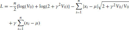
See the Appendix for a derivation of these results. The log-likelihood function L is given as follows:

4.2.5 Goodness of Fit of Marginal Distributions

Since we choose one of three distributions for the residuals of each issuer, we use four criteria to decide the best one. These are as follows:

• The Kolmogorov distance: This is defined as the supremum over the absolute differences between two cumulative density functions, the empirical one, F_emp(x), and the estimated fitted one, F_est(x).
• The Anderson and Darling Statistic: This is given by

The AD statistic puts more weight on the tails compared to the Kolmogorov statistic.

• The L¹ distance: This is equal to the average of the absolute differences between the empirical and statistical distributions.
• The L² distance: This is the root-mean-squared difference between the two distributions.

We use these criteria to choose between the normal, Student's t, and skewed double exponential distributions for each issuer. In each of our 56 simulated systems, the issuer level distributions are chosen from the following seven cases:

1. All marginal distributions were chosen to be normal.
2. All marginal distributions are Student's t.
3. All marginals are from the skewed double exponential family.
4. For each issuer, the best distribution is chosen based on the Kolmogorov criterion.
5. For each issuer, the best distribution is chosen based on the Anderson and Darling statistic.
6. Each marginal is chosen based on the best L¹ distance.
7. Each marginal is chosen based on the best L² distance.

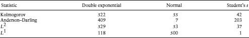
For each criterion, we count the number of times each distribution provides the best fit. The results are reported in Table 9.8, which provides interesting features. Based on the Kolmogorov, Anderson-Darling, and L² statistics, the skewed double exponential distribution is the most likely to fit the marginals best. However, the L¹ statistic finds that the normal distribution fits most issuers better. The better fit of the skewed double exponential as a marginal distribution comes from its ability to match the excess kurtosis of the distribution.

Table 9.8 In this table we report the Estimation Results of the Fit of Individual Intensity Residuals to Various Distributions. The three distributions chosen were: double exponential, normal, and the Student's t. We used four distance metrics to compare the empirical residuals to standardized distributions: the Kolmogorov distance, the Anderson–Darling statistic, and distances in the L¹ and L² norms. The table below presents the number of individual issuers that best fit each of the distributions under the different metrics. A total of 619 issuers was classified in this way.

4.3 Calibration

Our calibration procedure is as follows. First, using MLE, we determine the parameters of the various stochastic processes (rating-level averages and individual issuer PDs). Second, we choose one of the 56 possible correlation systems, as described above, and simulate the entire system 100 times to obtain an average simulated exceedance graph. Third, we compare the simulated exceedance graph with the empirical one (pointwise) and determine the mean-squared difference between the two graphs. This distance metric is used to determine a ranking of the 56 possible systems we work with.

5. SIMULATING CORRELATED DEFAULTS AND MODEL COMPARISONS

5.1 Overview

In this section, we discuss the simulation procedure. This step uses the estimated parameters from the previous section to generate correlated samples of hazard rates. The goal is for the simulation approach to deliver a model with the three properties described in the previous section. Therefore, the asymmetric correlation plot from simulated data should be similar to that in Figure 9.2.

We implement the simulation model with an additional constraint, whereby we ensure that the intensities (λ_k(t)) are monotonically increasing in rating level k. This prevents the average PD for a rating class from being lower than the average PD for the next better rating category; that is, λ_k(t) should be such that for all time periods t, it must be such that if i < j, then λ_i(t) < λ_j(t). This check is instituted during the simulation as follows. During the Monte Carlo step, if λ_i(t) > λ_j(t) when i < j, then we set λ_j(t) = λ_i(t). As an example, see Figure 9.3 where we plot the times series of λ_k, k = 1, …, 6 for a random simulation of the sample path of hazard rates.

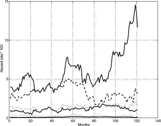
FIGURE 9.3 Simulated series of average PDs by rating class. The hazard rates are (from top to bottom of the graph) from rating class 6 to rating class 1. The simulation ensures that λ_i(t) < λ_j(t) if i < j.

5.2 Illustrative Monte Carlo Experiment

As a simple illustration that our approach arrives at a correlation plot fairly similar to that seen in the data, we ran a naive Monte Carlo experiment. In this exercise, we assumed that all error terms were normal, except under some conditions, when we assumed the Student's t distribution. We ran the Monte Carlo model 25 times and computed the average exceedance correlations for all rating classes. To obtain asymmetry in the correlations, we need to have higher correlations when hazard rates are high. To achieve this, the simulation uses the Student's t distribution with six degrees of freedom when the average level of hazard rates in the previous period in the simulation is above the empirical average of hazard rates. These features provided the results in Figure 9.4. The similarity between the empirical exceedance graph (Figure 9.2) and the simulated one (Figure 9.4) shows that the two-stage Monte Carlo model is able to achieve the three correlation properties of interest.

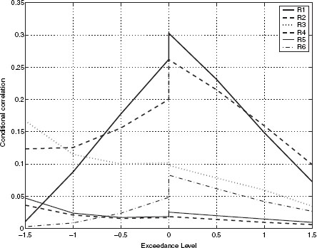
FIGURE 9.4 Asymmetric exceedance correlations of simulated PDs for the different rating classes. Again the plots are consistent with the presence of asymmetric correlation, and the degree of asymmetry is higher for the better rating categories.

5.3 Determining Goodness of Fit

The dependence structure among the intensities is depicted in the asymmetric correlation plots. We develop a measure to assess different specifications of the joint distribution. This metric is the average squared point-wise difference between the empirical exceedance correlation plot and the simulated one. The points in each plot that are used are for the combination of rating class (from 1 to 6) and exceedance levels (from −1.5 to +1.5). Hence, there is a total of 48 points in each plot that are used for computing the metric. Define the points in the empirical plot as h_k,x, where k indexes the rating class and x indexes the exceedance levels. The corresponding points in the simulated plot are denoted by h′_k,x. The metric q (a root-mean-squared estimation statistic) is as follows:

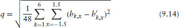
A smaller value of q implies a better fit of the joint dependence relationship. In the following section, we use the simulation approach and this metric to compare various models of correlated default.

5.4 Calibration Results and Metric

It is important to note that the joint dependence across all issuer intensities depends on three aspects: (1) the marginal distributions used for individual issuers, (2) the stochastic process used for each rating class, and (3) the copula used to implement the correlations between rating classes. Optimizing the choice of individual issuer marginal distributions will not necessarily achieve the best dependence relationship, because the copula chosen must also be compatible. In this chapter, we focus on four copulas (normal, Student's t, Gumbel, and Clayton), and allow the rating class intensity stochastic process to be either a jump-diffusion model or a regime-shifting model.

Tables 9.9 and 9.10 provide a comparison of the jump and the regime-switching models across copulas. Twenty-eight systems use a jump-diffusion model for the average PDs in each rating, and 28 use a regime-switching model. We see that the values of the q metric are consistently smaller for the regime-switching model using all test statistics. This implies that the latter model provides a better representation of the stochastic properties among the issuer hazard rates. In particular, it fits the asymmetric correlations better.¹² We conclude that, for rating-level PDs, a regime-switching model performs better than a jump-diffusion model, irrespective of the choice of issuer process and copula.¹³

Table 9.9 Comparison of Metric q Values for Jump-Diffusion and Regime-Shifting Models across the Normal (Gaussian) and Gumbel Copulas. For each model we generate the asymmetric correlation plot and then compute the distance metric. The asymmetric correlations (the metric q) are computed for the following seven cases: normal distribution, Student's t distribution, skewed double exponential distribution, the combination of the best distributions based on Kolmogorov criterion, the combination of the best distributions based on the Anderson and Darling statistic, and the combination based on the L¹ and L² norms

Table 9.10 Comparison of Metric q Values for the Jump-Diffusion and Regime-Shifting Models across the Clayton and Student's t Copulas Metric for best correlated default model (Clayton and Student's t copulas): this table presents the summary statistic for the asymmetric correlation metric to determine the best simulation model. For each model we generate the asymmetric correlation plot and then compute the distance metric. The asymmetric correlations (the metric q) are computed for the following seven cases: normal distribution, Student's t distribution, skewed double-exponential distribution, the combination of the best distributions based on Kolmogorov criterion, the combination of the best distributions based on the Anderson and Darling statistic, the combination based on the L¹ and L² norms. Our metric comprises the average squared point-wise difference between the empirical exceedance correlation plot and the simulated one. This a natural distance metric. The points in each plot that are used are for the combination of rating class (from 1 to 6) and exceedance levels (from −1.5 to +1.5). Hence there are a total of 48 points in each plot which are used for computing the metric. Define the points in the empirical plot as h_k,x, where k indexes the rating class and x indexes the exceedance levels. The corresponding points in the simulated plot are denoted h′_k,x. The metric q (a RMSE statistic) is as follows:

We report the results for both models, the jump-diffusion set up and the regime-switching one, and two copulas, the Clayton and Student's t copulas

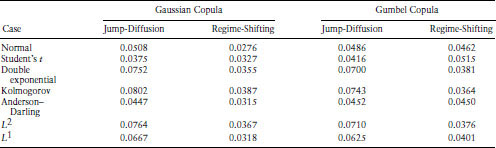
Tables 9.9 and 9.10 allow us to compare the fit provided by the four copulas. We find that when the jump-diffusion model is used, the Student's t copula performs best, no matter which marginal distribution is used. However, when the regime-switching model is used, sometimes the normal copula works best and at other times the Clayton copula is better. The normal copula works best when the marginals are all normal or Student's t, and when the marginals are chosen using the Anderson–Darling criterion. The Clayton copula is best when the marginals are all skewed double exponential or when the marginal criteria are Kolmogorov or L². The Student's t copula is best when the L¹ criterion is chosen.

These results bear some explanation. A comparison of the correlations from the skewed double exponential distribution with those from the raw data reveals that the model greatly overestimates the up-tail dependences. The Clayton copula decreases the up-tail dependences and increases the low-tail dependences. As a result, it corrects some of the overestimation from the double exponential marginals, resulting in better fitting. Hence, the Clayton copula seems to combine well with skewed double exponential marginals. On the other hand, the q metric favors the normal copula if the criterion chooses normal marginals (as with the normal, Student's t, and L¹ criteria), since less balancing of tail dependences is required.

5.5 Empirical Implications of Different Copulas

The degree of tail dependence varies with the choice of copula. It is ultimately an empirical question as to whether the parameterized joint distribution does result in differing tail risk in credit portfolios. To explore this question, we simulated defaults using a portfolio comprising all the issuers in this study under the regime-switching model. Remember that we fitted four copulas and seven different choices of marginal distributions, resulting in 28 different models, each with its attendant parameter set. To compare copulas, we fix the marginal distribution and then vary the copula.

As an illustration, we present Figure 9.5. This plots the tail loss distributions from the four copulas when all marginals are assumed to be normal. The line most to the right (the Gumbel copula) has the most tail dependence. There is roughly a 90% chance that the number of defaults will be less than 75; that is, a 10% probability that the number of defaults will exceed 75. For the same level of 75 defaults, the leftmost line (from the normal copula), there is only a 7% probability of the number of losses being greater than 75. By examining all four panels of the figure, we see that the ranking of copulas by tail dependence is unaffected by the choice of marginal distribution; that is, the normal copula is the leftmost plot, followed by the Student's t, Clayton, and Gumbel copulas.

Figure 9.6 In we plot the tail loss distributions for two models, the best fitting one and the worst. The best fit model combines the Clayton copula and marginal distributions based on the Kolmogorov criterion. The worst fit copula combines the Student's t copula with Student's t marginals. A comparison of the two models shows that the worst fitted copula in fact grossly overstates the extent of tail loss. Therefore, while there is tail dependence in the data, careful choice of copula and marginals is needed to avoid either under- or overestimation of tail dependence.

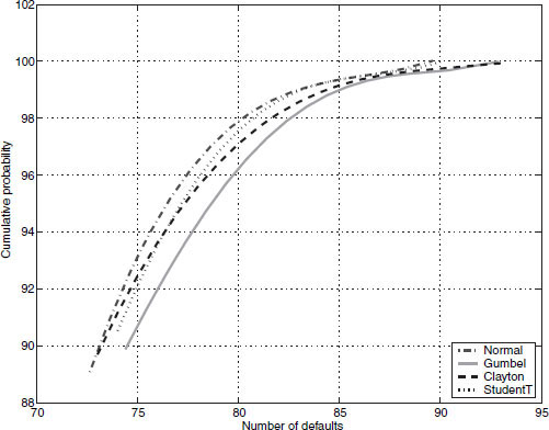
FIGURE 9.5 Comparison of copula tail loss distributions. This figure presents plots of the tail loss distributions for four copulas when the marginal distribution is normal. The x-axis shows the number of losses out of more than 600 issuers, and the y-axis depicts the percentiles of the loss distribution. The simulation runs over a horizon of 5 years and accounts for regime shifts as well. The copulas used are: normal, Gumbel, Clayton, Student's t.

6. DISCUSSION

This chapter develops a criterion-based methodology to assess alternative specifications of the joint distribution of default risk across hundreds of issuers in the US corporate market. The study is based on a data set of default probabilities supplied by Moody's Risk Management Services. We undertake an empirical examination of the joint stochastic process of default risk over the period 1987 to 2000. Using copula functions, we separate the estimation of the marginal distributions from the estimation of the joint distribution. Using a two-step Monte Carlo model, we determine the appropriate choice of multivariate distribution based on a new metric for the assessment of joint distributions.

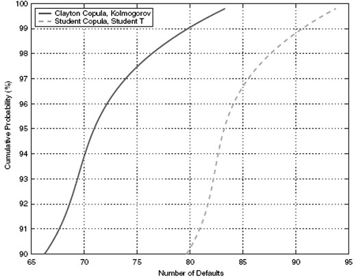
FIGURE 9.6 Comparison of copula tail loss distributions: in this figure we plot the tail loss distributions for two models, the best fitting one and the worst. The best fit model combines the Clayton copula and marginal distributions based on the Kolmogorov criterion and the worst fit copula combines the Student's t copula with Student's t marginals. The simulation runs over a horizon of 5 years and accounts for regime shifts as well.

We explore 56 different specifications for the joint distribution of default intensities. Our methodology uses two alternative specifications (jumps and regimes) for the means of default rates in rating classes. We consider three marginal distributions for individual issuer hazard rates, combined using four different copulas. An important extension to this model structure is the inclusion of rating changes. In our analysis, we centered firms as lying within the same rating for the period of the simulation, based on their most prevalent rating. The two-step simulation model would need to be enhanced to a three-step one, with an additional step for changes in ratings.¹⁴

Other than the myriad specifications, there are many useful features of the analysis for modelers of portfolio credit risk. First, we develop a simple metric to measure best fit of the joint default process. This metric accounts for different aspects of default correlation—namely, level, asymmetry, and tail dependence or extreme behavior. Second, the simulation model, based on estimating the joint system of over 600 issuers, is able to replicate the empirical joint distribution of default. Third, a comparison of the jump model and the regime-switching model shows that the latter provides a better representation of the properties of correlated default. Fourth, the skewed double exponential distribution is a suitable choice for the marginal distribution of each issuer hazard rate process, and combines well with the Clayton copula in the joint dependence relationship among issuers. Our simulation approach is fast and robust, allowing for rapid generation of scenarios to assess risk in credit portfolios. Finally, the results show that it is important to correctly capture the interdependence of marginal distributions and copula to achieve the best joint distribution depicting correlated default. Thus, this chapter delivers the empirical counterpart to the body of theoretical papers advocating the usage of copulas in modeling correlated default.

ACKNOWLEDGMENTS

We are extremely thankful for many constructive suggestions and illuminating discussions with Darrell Duffie, Gifford Fong, Nikunj Kapadia, John Knight, and Ken Singleton, and participants at the Q-conference (Arizona 2001), Risk Conference (Boston 2002), and Barclay's Global Investors Seminar (San Francisco 2002). We are also very grateful to two excellent (anonymous) prior referees for superb comments and guidance that resulted in a much-transformed chapter. The first author gratefully acknowledges support from the Dean Witter Foundation and a Breetwor Fellowship. We are also grateful to Gifford Fong Associates and Moody's Investors Services for data and research support for this chapter. The second author is supported by the Natural Sciences and Engineering Research Council of Canada.

APPENDIX: THE SKEWED DOUBLE EXPONENTIAL DISTRIBUTION

Assume that a random variable X has a normal distribution with mean μ + γV and variance V, where V has an exponential distribution with the following density function:

Then X has a skewed double exponential distribution.

A.1 Density Function

The density function is derived as follows:

A.2 Maximizing the Log-Likelihood Function

This subsection deals with the technical details of the maximization of log-likelihoods for the skewed double exponential model. The likelihood function is

where m is the number of observations in which x_i is greater than μ, l is the number of observations otherwise, and n = m + l.

The first-order condition can be derived as follows:

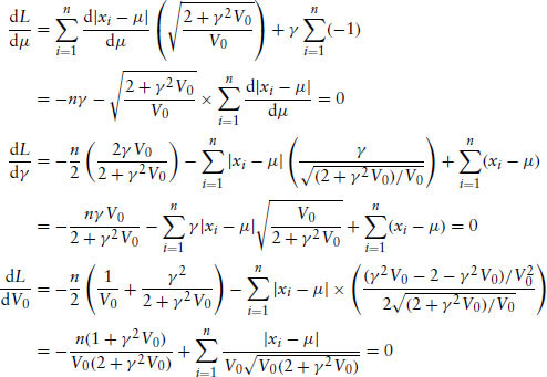
Solving the above first-order conditions gives

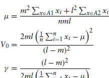
where A1 = {x : x_i – μ ≥ 0} and A2 = {x : x_i – μ < 0}.

Given a dataset, we may not be able to find a value of μ to satisfy the above equations. However, by choosing μ to be as close as given by the first-order conditions, we can fit the data well with the skewed double exponential distribution.

NOTES

1. See the structural models of Merton (1974), Geske (1977), Leland (1994), and Longstaff and Schwartz (1995); and the reduced-form models of Duffie and Singleton (1999), Jarrow and Turnbull (1995), Das and Tufano (1996), Jarrow et al. (1997), Madan and Unal (1999), and Das and Sundaram (2000).

2. A CDO securitization comprises a pool of bonds (the “collateral”) against which tranches of debt are issued with varying cash flow priority. Tranches vary in credit quality from AAA to B, depending on subordination level. Seller's interest is typically maintained as a final equity tranche, carrying the highest risk. CDO collateral usually comprises from a hundred to over a thousand bond issues. Tranche cash flows critically depend on credit events during the life of the CDO, requiring Monte Carlo simulation [see, for example, Duffie and Singleton (1999)] of the joint default process for all issuers in the collateral. An excellent discussion of the motivation for CDOs and the analysis of CDO value is provided in Duffie and Garleanu (2001). For a parsimonious model of bond portfolio allocations with default risk, see Wise and Bhansali (2001).

3. As demonstrated by Das et al. (2001b) and by Gersbach and Lipponer (2000), both the individual default probability and the default correlations have a significant impact on the value of a credit portfolio.

4. Extreme value distributions allow for the fact that processes tend to evidence higher correlations when tail values are experienced. This leads to a choice of fatter-tailed distributions with a reasonable degree of “tail dependence.” The support of the distribution should also be such that the PD intensity λ_i(t) lies in the range [0, ∞).

5. There is a growing literature on copulas. The following references contain many useful papers on the topic: Embrechts et al. (1997), Embrechts et al. (1999a,b), Frees and Valdez (1998), Frey and McNeil (2001a,b), Li (1999), Nelsen (1999), Lindskog (2000), Schonbucher and Schubert (2001), and Wang (2000).

6. Durrleman et al. (2000) discuss several parametric and non-parametric copula estimation methods.

7. Lower tail dependence is symmetrically defined. The coeffcient of lower tail dependence

If λ_L > 0, then lower tail dependence exists.

8. This specification does permit the hazard rate to populate negative values. While this is not an issue during the estimation phase, the simulation phase is adjusted to truncate the shock if the negative support is accessed. However, we remark that this occurs in very rare cases, since λ_k(t) is the average across all issuers within the rating class, and the averaging drives the probability of negative hazard rates to minuscule levels.

9. Ang and Chen (2002) found this type of model to be good at capturing the three stated features of asymmetric correlation in equity markets.

10. We found that the estimations of θ_r were very sensitive to the initial values used in the optimization. By fixing these two values, the estimation turned out to be more stable.

11. The estimation of equation 9.11 relies on the assumption that the mean around which the individual hazard rate oscillates depends on the initial rating class of the issuer, even though this may change over time. Extending the model to map default probabilities to rating classes is a nontrivial problem, and would complicate the estimation exercise here beyond the scope of this chapter. Indeed, this problem in isolation from other estimation issues is complicated enough to warrant separate treatment and has been addressed in a chapter by Das et al. (2002).

12. This result is consistent with that of Ang and Chen (2002), who undertake a similar exercise with equity returns.

13. The fact that the Student's t marginal distribution works best for the jump models may indicate that the jump model does not capture the dependences as well as the regime-switching model does, since the Student's t distribution is good at injecting excess kurtosis into the conditional distribution of the marginals.

14. We are grateful to Darrell Duffie for this suggestion.

REFERENCES

Abramowitz, M. and Stegun, I. A. (1972). The Handbook of Mathematical Functions. New York: Dover.

Ang, A. and Chen, J. (2002). “Asymmetric Correlation of Equity Portfolios.” Journal of Financial Economics 63(3), 443–494.

Bouye, E., Durrleman, V., Nikeghbali, A., Riboulet, G. and Roncalli, T. (2000). “Copulas for Finance: A Reading Guide and Some Applications.” Working Paper, Credit Lyonnais, Paris.

Clayton, D. G. (1978). “A Model for Association in Bivariate Life Tables and Its Application in Epidemiological Studies of Familial Tendency in Chronic Disease Incidence.” Biometrika 65, 141–151.

Crouhy, M., Galai, D. and Mark, R. (2000). “A Comparative Analysis of Current Credit Risk Models.” Journal of Banking and Finance 24, 59–117.

Das, S., Fan, R. and Geng, G. (2002). “Bayesian Migration in Credit Ratings Based on Probabilities of Default.” Journal of Fixed Income 12(3), 17–23.

Das, S., Freed, L., Geng, G. and Kapadia, N. (2001a). “Correlated Default Risk.” Working Paper, Santa Clara University.

Das, S., Fong, G. and Geng, G. (2001b). “The Impact of Correlated Default Risk on Credit Portfolios.” Journal of Fixed Income 11(3), 9–19.

Das, S. and Sundaram, R. (2000). “A Discrete-Time Approach to Arbitrage-Free Pricing of Credit Derivatives.” Management Science 46(1), 46–62.

Das, S. and Tufano, P. (1996). “Pricing Credit Sensitive Debt When Interest Rates, Credit Ratings and Credit Spreads Are Stochastic.” The Journal of Financial Engineering 5(2), 161–198.

Das, S. and Uppal, R. (2000). “Systemic Risk and International Portfolio Choice.” Working Paper, London Business School.

Davis, M. and Violet, L. (1999a). “Infectious Default.” Working Paper, Imperial College, London.

Davis, M. and Violet, L. (1999b). “Modeling Default Correlation in Bond Portfolios.” In C. Alexander (ed.) ICBI Report on Credit Risk.

Dowd, K. (1999). “The Extreme Value Approach to VaR: An Introduction.” Financial Engineering News 3(11).

Duffie, D. J. and Garleanu, N. (2001). “Risk and Valuation of Collateralized Debt Obligations.” Financial Analysts Journal 57(1), 41–59.

Duffie, D. J. and Singleton, K. J. (1999). “Simulating Correlated Defaults.” Working Paper, Stanford University, Graduate School of Business.

Durrleman, V., Nikeghbali, A. and Roncalli, T. (2000). “Which Copula Is the Right One?” Working Paper, Groupe de Recherche Operationnelle, Credit Lyonnais, France.

Embrechts, P., Kluppelberg, C. and Mikosch, T. (1997). Modeling Extremal Events for Insurance and Finance. Berlin: Springer-Verlag.

Embrechts, P., McNeil, A. and Straumann, D. (1999a). “Correlation and Dependence in Risk Management: Properties and Pitfalls.” Working Paper, University of Zurich.

Embrechts, P., McNeil, A. and Straumann, D. (1999b). “Correlation: Pitfalls and Alternatives.” Working Paper, Department Mathematik, ETH Zentrum, Zurich.

Embrechts, P., Lindskog, F. and McNeil, A. (2001). “Modeling Dependence with Copulas and Applications to Risk Management.” Working Paper CH-8092, Dept. of Mathematics, ETZH Zurich.

Frees, E. W. and Valdez, E. A. (1998). “Understanding Relationships Using Copulas.” North American Actuarial Journal 2(1), 1–25.

Frey, R. and McNeil, A. J. (2001a). “Modeling Dependent Defaults.” Working Paper, University of Zurich.

Frey, R. and McNeil, A. J. (2001b). “Modeling Dependent Defaults: Asset Correlation Is Not Enough.” Working Paper, University of Zurich.

Genest, C. (1987). “Frank's Family of Bivariate Distributions.” Biometrika 74, 549555.

Genest, C. and Rivest, L. (1993). “Statistical Inference Procedures for Bivariate Archimedean Copulas.” Journal of the American Statistical Association 88, 1034–1043.

Gersbach, H. and Lipponer, A. (2000). “The Correlation Effect.” Working Paper, University of Heidelberg.

Geske, R. (1977). “The Valuation of Corporate Liabilities as Compound Options.” Journal of Financial and Quantitative Analysis 12(4), 541–552.

Gumbel, E. J. (1960). “Distributions des valeurs extremes en plusiers dimensions.” Publ. Inst. Statist. Univ. Paris 9, 171–173.

Jarrow, R. A. and Turnbull, S.M. (1995). “Pricing Derivatives on Financial Securities subject to Credit Risk.” Journal of Finance 50(1), 53–85.

Jarrow, R. A., Lando, D. and Turnbull, S. M. (1997). “A Markov Model for the Term Structure of Credit Spreads.” Review of Financial Studies 10, 481–523.

Jarrow, R. A. and Yu, F. (2000). “Counterparty Risk and the Pricing of Defaultable Securities.” Working Paper, Johnson GSM, Cornell University.

Kijima, M. (2000). “Credit Events and the Valuation of Credit Derivatives of Basket Type.” Review of Derivatives Research 4, 55–79.

Lee, A. J. (1993). “Generating Random Binary Deviates Having Fixed Marginal Distributions and Specified Degree of Association.” The American Statistician 47, 209–215.

Leland, H. E. (1994). “Corporate Debt Value, Bond Covenants and Optimal Capital Structure.” Journal of Finance 49(4), 1213–1252.

Li, D. X. (1999). “On Default Correlation: A Copula Function Approach.” Working Paper 99–07, The Risk Metrics Group, New York.

Lindskog, F. (2000). “Modeling Dependence with Copulas and Applications to Risk Management.” Working Paper, Risklab, ETH Zurich.

Longin, F. and Solnik, B. (2001). “Extreme Correlation of International Equity Markets.” Journal of Finance 56, 649–676.

Longstaff, F. A. and Schwartz, E. S. (1995). “A Simple Approach to Valuing Risky Fixed and Floating Rate Debt.” Journal of Finance 50(3), 789–819.

Madan, D. and Unal, H. (1999). “Pricing the Risks of Default.” Review of Derivatives Research 2(2/3), 121–160.

Merton, R. (1974). “On the Pricing of Corporate Debt: The Risk Structure of Interest Rates.” Journal of Finance 29, 449–470.

Nelsen, R. B. (1999). An Introduction to Copulas. New York: Springer-Verlag. Sklar, A. (1959). “Functions de repartition a n dimensions et leurs marges.” Publ. Inst. Statist. Univ. Paris 8, 229–231.

Sklar, A. (1973). “Random Variables, Joint Distributions, and Copulas.” Kybernetica 9, 449–460.

Schonbucher, P. and Schubert, D. (2001). “Copula-Dependent Default Risk in Intensity Models.” Working Paper, Dept. of Statistics, Bonn University.

Wang, S. S. (2000). “Aggregation of Correlated Risk Portfolios: Models and Algorithms.” Working Paper, CAS.

Wise, M. and Bhansali, V. (2001). “Portfolio Allocation to Corporate Bonds with Correlated Defaults.” Working Paper No. CALT-68-2365, California Institute of Technology.

Xiao, J. (2003). “Constructing the Credit Curves: Theoretical and Practical Considerations.” Working Paper, Risk Metrics.

Zhou, C. (2001). “An Analysis of Default Correlations and Multiple Default.” Review of Financial Studies 14, 555–576.

Keywords: Correlated default; copulas; tail dependence

---

^aSanta Clara University, Santa Clara, CA 95053.

^bAmaranth Group Inc., Greenwich, CT 06831.

^*Corresponding author. Santa Clara University, Santa Clara, CA 95053, USA. E-mail: [email protected].