CHAPTER 1

Estimating Default Probabilities Implicit in Equity Prices

Tibor Janosi,^a Robert Jarrow,^b,* and Yildiray Yildirim^c

1. INTRODUCTION

Given the recent exponential growth in the credit derivatives market (see Risk Magazine, 2000), credit risk modeling and estimation have become topics of interest. The theoretical literature is quite extensive (see Bielecki and Rutkowski, 2000, for a review). The empirical literature estimating reduced-form credit risk models has concentrated on using debt prices (see Duffie, 1999; Duffie and Singleton, 1997; Duffie et al., 2000; Janosi et al., 2002; Madan and Unal, 1998), credit derivative prices (see Hull and White, 2000, 2001), or bankruptcy histories (see Altman, 1968; Chava and Jarrow, 2002; Shumway, 2001; Zmijewski, 1984). Equity prices have only been used to estimate default parameters for structural models (see Delianedis and Geske, 1998). The purpose of this chapter is to use equity prices in conjunction with a reduced form credit risk modeling approach to estimate default probabilities. The approach utilized is a slight generalization of the model contained in Jarrow (2001).

The data used for this investigation are equity prices from the Center for Research in Security Prices (CRSP) and debt prices from the University of Houston's Fixed Income Database over the time period May 1991-March 1997. The observation interval is 1 month. Debt prices consist of bids taken from Lehman Brothers trading sheets on the last calendar day in each month, see Warga (1999) for additional details.

Fifteen different firms are included in this study, where the firms are chosen to stratify various industry groupings: financial, food and beverages, petroleum, airlines, utilities, department stores, and technology. The same 15 firms as in Janosi et al. (2002) are included so that a comparison of the different estimation procedures can be performed.

Eight different models for equity returns are investigated herein, the simplest models containing no default. Using a rolling estimation procedure for each month during this observation period, the equity model's parameters (including the bankruptcy parameters) are estimated using a time-series regression on monthly equity returns. In this procedure, only information available to the market at the time the equations are estimated is utilized.

First, the analysis supports the feasibility of estimating default probabilities implicit in equity returns. In a relative comparison of the eight models, in-sample root mean squared error goodness-of-fit tests and out-of-sample generalized cross-validation statistics support the necessity of including default parameters into the equity return model. The best performing default intensity depends on the spot rate of interest but not on an equity market index, confirming similar results that Janosi et al. (2002) obtained when using debt prices.

Second, we find that equity returns contain a bubble component not captured by the Fama and French (1993,1996) four-factor model for equity's risk premium. This bubble component, proxied by the firm's P/E ratio, is significant for many of the firms in our sample.

Third, due to the possible existence of equity price bubbles and the difficulty in modeling equity risk premium, the default intensity estimates obtained appear to confound these quantities. Indeed, a comparison of the default intensity estimates obtained herein with those obtained using either historical data or implicitly from debt prices indicates that the equity-based default intensities are significantly larger. By extrapolation, this possible model misspecification also casts doubt on the reliability of the equity-based default probability estimates obtained using structural models as in Delianedis and Geske (1998), confirming the previous conclusions of Jarrow and van Deventer (1998, 1999) and Jarrow et al. (2002) in this regard. This is also consistent with the inability of structural models, using equity price information, to explain credit spreads in corporate debt; see Collin-Dufresne et al. (2001), Eom et al. (2002), and Huang and Huang (2002).

The previous literature estimating reduced-form credit risk models using debt prices includes Duffie (1999), Duffie and Singleton (1997), Duffie et al. (2000), Janosi et al. (2002), and Madan and Unal (1998). Duffie and Singleton (1997) estimate swap spreads, Madan and Unal (1998) estimate yields on thrift institution certificates of deposit, and Duffie et al. (2000) estimate credit and liquidity spreads for Russian debt. Both Duffie (1999) and Janosi et al. (2002) estimate default intensities using US corporate debt. As mentioned earlier, we will compare our estimated default intensities with those from Janosi et al. (2002). Bankruptcy prediction models using historical bankruptcy data include Altman (1968), Chava and Jarrow (2002), Shumway (2001), and Zmijewski (1984), among others. A structural model for estimating default intensities is Delianedis and Geske (1998).

An outline of this chapter is as follows. Section 2 presents the model structure. Section 3 provides a description of the data, and Section 4 estimates the state variable process parameters. The equity model parameter estimation is discussed in Sections 5–10;. Section 11 compares the default parameter intensities estimated using the equity model to those obtained using debt prices by Janosi et al. (2002). A conclusion is provided in Section 12.

2. THE MODEL STRUCTURE

This section introduces the notation and provides a generalization of the reduced-form credit risk model for equity returns contained in Jar-row (2001). Default-free zero-coupon bonds of all maturities and a firm's common stock are traded. Markets are assumed to be frictionless with no arbitrage opportunities, but equity prices may contain bubbles.

Let p(t, T) represent the time t price of a default-free dollar paid at time T where 0 ≤ t ≤ T. The instantaneous forward rate at time t for date T is defined f (t, T) = – ∂ log p(t, T)/∂T, with the spot rate of interest r(t) = f(t, t).

Consider a firm issuing equity. This firm may default. Let τ be the random variable representing the first time of default and let

denote its point process. We assume that this point process has an intensity, denoted by λ(t). λ(t) Δ gives the approximate probability of the firm's default over the time interval [t, t + Δ].¹

Equity pays dividends and has a liquidating payoff at time T_L. The time t value of all of these payments equals the value of the equity (per share), denoted by ξ(t). These promised dividends and liquidating payoff are made, unless the firm defaults. If default occurs, the equity holders lose everything.²

We need to develop some notation for these promised payments to equity. The regular dividends D_t are paid at times t = 1,2,…, T_D. We assume that these dividends are deterministic quantities, placed in an escrow account and paid for sure.³ The requirement that these dividends are deterministic implicitly determines the date T_D. For many equities, T_D will be a month or less. The liquidating dividend L(T_L) is paid at time T_L unless default occurs prior to this date. The liquidating dividend consists of the time T_L (future) value of all unannounced and random dividends paid over (T_D, T_L), plus the remaining resale value of the firm at time T_L.

Let S(t) represent the time t present value of the liquidating dividend, conditional upon no default prior to time t. There is some evidence for example, the recent price growth of Internet stocks⁴, that stock prices contain a “bubble” or “monetary value” component; see Jarrow and Madan (2000). For simplicity, we model the bubble component as a random process that is proportional to the present value of the liquidating dividend:

where μ_θ (u) ≥ 0 is the continuous return in the stock price due to the bubble component.

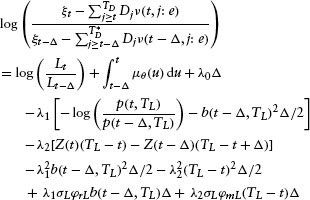
Given this set-up, it is easy to see⁵ that the per share equity value at time t is given by

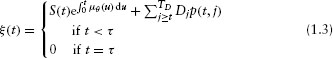
The share price consists of the present value of the liquidating dividend (S(t)) compounded by the bubble (μ_θ (t)), and the (announced) deterministic dividends (D_j for j = t,…,T_D).

To obtain an empirical formulation of the above model, more structure needs to be imposed on the stochastic nature of the economy. Exactly following Jarrow (2001),⁶ we consider an economy that is Markov in three state variables: the spot rate of interest, the cumulative excess return on an equity market index, and the liquidating dividend process. For the spot rate of interest, we use a single-factor model with deterministic volatilities, sometimes called the extended Vasicek model. This model has two parameters: a mean reversion parameter (a) and the spot rate's volatility (σ_r). The second state variable Z(t) is the cumulative excess return on an equity market index. The equity market index follows a geometric Brownian motion with volatility (σ_m). The correlation coefficient between the return on the market index and changes in the spot rate of interest is (φ_rm). The third state variable is the liquidation value of the firm's equity, denoted by L(t). This liquidation value is assumed to follow a geometric Brownian motion with volatility (σ_L) and with φ_mL and φ_rL representing the correlation of the liquidation value with the market index and changes in the spot rate of interest, respectively.

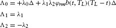
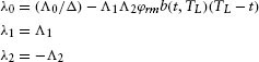
For analytic tractability, the default intensity process is assumed to be linear in the spot rate of interest and the cumulative excess return on the equity market index; that is,

where λ₀, λ₁, λ₂ are constants.

Under this structure, it is shown in Jarrow (2001) that the present value of the liquidating dividend can be rewritten as

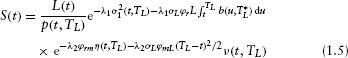
where

and

Substitution of equation 1.5 into the stock price equation 1.3 yields the final valuation formula.

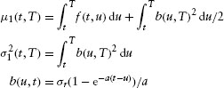
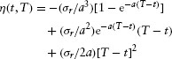
Unfortunately, observing only a single value for the stock price at each date leaves this system underdetermined as there are more unknowns (L(t), λ₀, λ₁, λ₂) than there are observables (ξ(t)).⁷ To overcome this situation, the stochastic process for L(t) is used to transform equation 1.3 into a time-series model for the firm's equity returns. Unfortunately, this transformation introduces the equity price's risk premium into the estimation procedure. In this regard, it is shown in the appendix that⁸

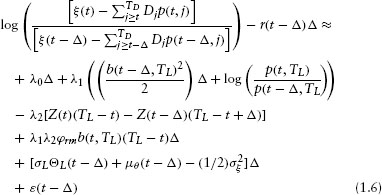
where ε(t – Δ) ≡ σ_L(w_L(t) – w_L(t – Δ)) and Θ_L(t) is the liquidation value's risk premium.

Equation 1.6 gives a time-series expression for the stock's return over the time period [t – Δ, t]. This is a generalization of the typical asset-pricing model to include a firm's default parameters. This expression forms the basis for our empirical estimation in the subsequent sections.

One can think of this model for equity returns in three different but related ways. The first interpretation of equation 1.6 is that it is equivalent to a reduced-form credit risk model for the firm's equity. This interpretation follows the method of derivation. The second interpretation of equation 1.6 is that it is a type of structural model for the firm's equity where the firm's liquidation value (assets less liabilities) is exogenously given and default occurs according to a default intensity process correlated with the randomness inherent in the firm's liquidation value. Finally, the third interpretation of equation 1.6 is that it is a generalized asset-pricing model with bankruptcy explicitly parameterized within the equity's return process. Given this perspective, equation 1.6 makes explicit the bond market factor discussed in Fama and French (1993).

3. DESCRIPTION OF THE DATA

The time period covered in this study is May 1991–March 1997. The interval for computing equity returns is 1 month. For each firm, and for each month in the observation period, we will be fitting a time-series regression of equity returns going back in time 4 years (48 months). Thus, we lose the first 4 years of our observation interval, giving time-series regressions for each firm and for each month from May 1995–March 1997.

All individual firm equity data (including earnings, dividends, etc.) are obtained from CRSP. For the equity market index, we used the S&P 500 index. For estimating an equity risk premium, we will employ the Fama–French benchmark portfolios (book-to-market factor (HML), small firm factor (SMB), and a momentum factor (UMD). These monthly portfolio returns were obtained from Ken French's webpage.⁹

The US Treasury prices used for this investigation were obtained from the University of Houston's Fixed Income Database. The data consist of monthly bid prices of all outstanding bills, notes, and bonds taken from Lehman Brothers' trading sheets on the last calendar day in each month; see Warga (1999) for additional details. Being such a large database (containing over two million entries), the potential for data errors is quite large. Indeed, a careful examination of the data confirmed this suspicion. Hence, we filtered the data to remove obvious data errors. We excluded Treasury bonds with inconsistent or suspicious issue/dated/maturity dates and matrix prices. Lastly, using a median yield filter of 2.5%, we also removed US Treasury debt listings whose yields exceeded the median yield by this percent. After filtering, there are approximately 29,100 US Treasury prices left in the sample set.

The same 20 firms as in Janosi et al. (2002) were initially selected for analysis. These firms were selected to stratify various industry groupings: financial, food and beverages, petroleum, airlines, utilities, department stores, and technology. Due to unavailability of balance sheet data or stock prices, five of these companies were eliminated. The remaining 15 firms included in this study and the industry represented by each firm are provided in Table 1.1. The Moody's and S&P ratings for each company's debt issues at the start of our sample period (May 24, 1991) are also included.

As mentioned previously, the interval for equity returns is 1 month. The monthly return interval was chosen for two reasons. First, the default parameter estimation using debt prices in Janosi et al. (2002) was based on monthly data, so monthly equity returns will provide an equivalent comparison. Second, and more importantly, it is believed that the use of monthly data for equities eliminates market-microstructure noise more prevalent in smaller return intervals (daily or weekly) (see Dimson, 1979; Schwartz and Whitcomb, 1977a,b; Smith, 1978).

Table 1.1 Details of the Firms Included in the Empirical Investigation

4. ESTIMATION OF THE STATE VARIABLE PROCESS PARAMETERS

To implement the estimation of the equity return process, we use a two-step procedure. In step one, we first estimate the parameters for the state variable processes. Step two uses these estimates as constants in the equity return estimation. Step two is discussed in Section 5.

4.1 Spot Rate Process Parameter Estimation

The inputs to the spot rate process evolution are the forward rate curves over an extended observation period (f (t, T) for all months t ∈ January 1975–March 1997) and the spot rate parameters (a, σ_r).

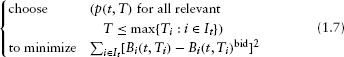
For the estimation of the forward rate curves, a two-step procedure is also utilized. First, for a given time t, the discount bond prices (p(t, T) for various T) are estimated by solving the following minimization problem:

where

is a US Treasury security with coupons of C_j dollars at times t_j for j = 1,…, n_i, where t_ni = T_i is the maturity date; I_t is an index set containing the various US Treasury bonds, notes, and bills available at time t; and B_i(t, T_i)^bid is the market bid price for the ith bond with maturity T_i.

The discount bond prices' maturity dates T coincide with the maturities of the Treasury bills, and the coupon payment and principal repayment dates for the Treasury notes and bonds.

Step 2 is to fit a continuous forward rate curve to the estimated zero-coupon bond prices (p(t, T) for all T ≤ max{T_i: i ∈ I}). We use the maximum smoothness forward rate curve as developed by Adams and van Deventer (1994) and refined by Janosi and Jarrow (2002). Briefly, we choose the unique piecewise, fourth-degree polynomial with the left and right end points left “dangling” that minimizes

For the estimation of the spot rate parameters (a, σ_r), the procedure follows that used in Janosi et al. (2002). A rolling estimation of the parameters using only information available at the time of the estimation is performed, making the parameter estimates (a_t, Δ_rt) dependent on time t as well. The procedure is based on an explicit formula for the variance of the default-free zero-coupon bond prices under the extended Vasicek model (see Heath et al., 1992). For Δ = 1/12 (a month), the expression is

First, we fix a time to maturity T – t ∈ {3 months, 6 months, 1 year, 5 years, 10 years, the longest time to maturity of an outstanding Treasury bond closest to 30 years}. Then, we fix a current month t ∈ {May 1991–March 1997}. Going backward in time 60 months (5 years), we compute the sample variance, denoted v_tT, using the smoothed forward rate curves previously generated. Note that the sample variance depends on both the date of estimation and the bond's maturity. Then, for each month t ∈{May 1991–March 1997}, to estimate the parameters (σ_rt, a_t) we run a nonlinear regression

across the bond time to maturities T – t ∈{1/4, 1/2, 1, 5, 10, longest time to maturity closest to 30} where e_tT is the error term.

The parameter estimates are

The R² for each of these monthly nonlinear regressions (not reported) exceeded 0.99 in all cases. The spot rate volatility (σ_rt) is nearly constant over this period. In contrast, the mean reverting parameter (a_rt) appears to be more volatile.

To test for the time-series stability of these parameter estimates, a unit root test was performed.¹⁰ For the volatility σ_rt, the test rejects a unit root, implying the time series is stationary. In contrast, one cannot reject a unit root for the mean reverting parameter a_t.

4.2 Market Index Parameter Estimation

Although the equity returns are monthly, for estimating the parameters of the market index we use daily data. This is done because daily data are available for the market index, and the higher frequency data will provide less noisy estimates because market microstructure considerations are less important for an index (than they are for individual firms). Daily observations of the market return and the 3-month T-bill yield are available from CRSP. Using the daily S&P 500 index price data and the daily 3-month T-bill spot rate data, we estimate the parameters of the market index process (σ_m, φ_rm).

As previously mentioned, this estimation is based on daily data (Δ = 1 /365). As before, the procedure involves a rolling estimation of the parameters using only information available at the time of the estimation. For a given day t ∈ {May 24,1990–March 31,1997}, we go back in time 365 business days and estimate the time-dependent sample variance and correlation coefficients (σ_mt, φ_rmt) using the sample moments, that is

and

The parameter estimates are

The market volatility is relatively constant between 0.1 and 0.2 over this observation period. The correlation coefficient appears to be more variable. As before, to test for the stability of the parameters a unit root test was performed. The results show that a unit root can be rejected at the 90% confidence level for the market volatility but not for the correlation coefficient.¹¹

With the parameter estimates for the market volatility (σ_mt) and the daily 3-month Treasury bill yields, the excess cumulative return on the market process Z(t) is computed,¹² starting the time series on May 24, 1991.

5. EQUITY RETURN ESTIMATION

Given the state variable parameters as estimated in the previous sections, this section presents the estimated equity return model. The basis for this estimation is equation 1.6. To empirically implement equation 1.6, we need to specify models for both the risk premium and the equity price bubble.

Following Fama and French (1993, 1996), we use a four-factor asset-pricing model with the factors being the excess return on a market portfolio, SMB(t), HML(t), and UMD(t), that is,

where SMB(t) is the difference between the return on a portfolio of small stocks and the return on a portfolio of large stocks at time t, HML(t) is the difference between the return on a portfolio of high-book-to-market stocks and the return on a portfolio of low-book-to-market stocks at time t, and UMD(t) is a momentum factor.

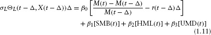
The equity price bubble is proxied by the price-earnings ratio and possibly the stock's own variance, that is,

where

The stock's own variance is included with an arbitrary coefficient to see if it differs from its theoretical value of –(1/2) in equation 1.6. There is also a concern that the SMB(t), HML(t), and UMD(t) factors may already include an adjustment for bubbles. For this reason, the subsequent regressions are run both with and without the P/E ratio included.

For the estimation, we fix (T_L – t) = 20 years and we set T_D = t. The first restriction makes the firm's valuation horizon 20 years, making equity comparable with long-term debt. The second restriction implies that all future dividends are viewed as random. Consequently, we only need to make an adjustment for dividends in the payout month.

Substitution of the above into equation 1.6 yields:

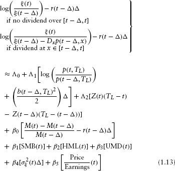
where

To ensure that the intensity process is non-negative when both λ₁ and λ₂ are zeros, we impose the constraint that Λ₀ ≥ 0 in the estimation. The final computations for the default parameters are

The time period covered is May 1991–March 1997. For each firm, a time-series regression is run using 48 months of historical data. Thus, the first regression estimation occurs 4 years into the data set on May 31, 1995. For each subsequent month, until March 1997, the regression is re-estimated and parameter estimates obtained. This generates 23 regressions for each firm's returns. As before, only information available to the market at the time of the estimation is utilized. This rolling estimation procedure gives a monthly time series of parameter estimates (λ_0t,λ_1t, λ_2t, β_0t, β_1t, β_2t, β_3t, β_4t, β_5t) based on 46 (48–2;) months of overlapping data. The choice of a 4-year estimation period was based on trading off the stability of the estimates versus larger standard errors. Although longer estimation periods are likely to make the standard errors smaller, they also imply that structural shifts are more likely to occur, making the estimated parameters less stable.

Eight different models for equity returns are estimated. The models differ with respect to the number of independent variables included in the regression. Models 1 and 2 have no default (λ₀ ≡ λ₁ ≡ λ₂ ≡ 0). They differ only in the inclusion of a P/E ratio (β₅ ≡ 0 or not). Models 3–8 include default, and they differ with respect to the default intensity investigated and the inclusion of the P/E ratio or not. In particular, models 3 and 4 have only λ0 nonzero. Models 5 and 6 have both λ₀ and λ₁ nonzero. Models 7 and 8 have all default parameters nonzero. These eight models are nested and a relative comparison of model performance is subsequently provided.

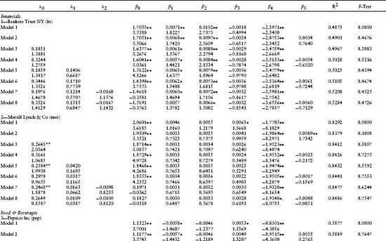
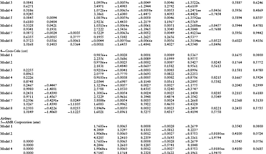
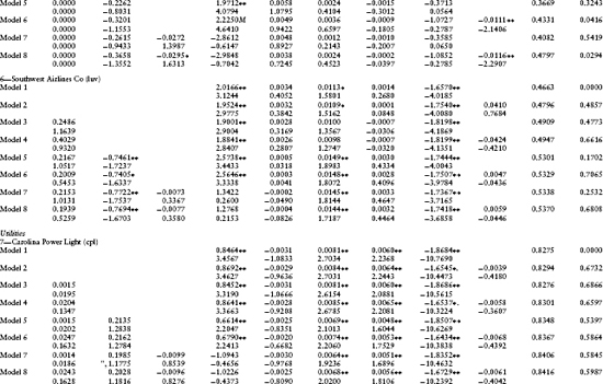
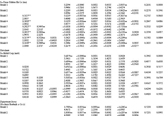
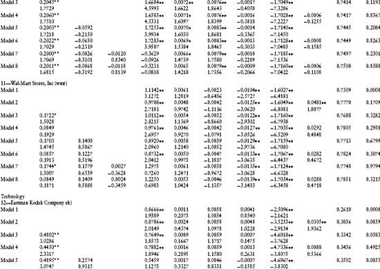
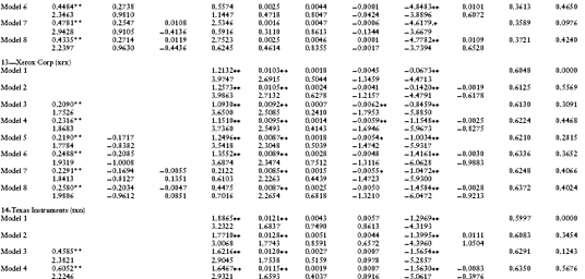
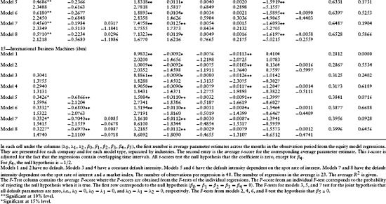
To summarize the monthly time series estimates across all models and across all times, Table 1.2 provides the average values for the point estimates of the parameters and their t-statistics.¹³ The average adjusted R² is also included. The values in Table 1.2 are averages over the number of months in the observation period (May 1995–March 1997) for which the linear regression estimates of the parameters are computed.¹⁴ Summary statistics for various F-tests are also provided. The first F-test is for the null hypothesis (β_0t = β_1t = β_2t = β_3t = β_4t = 0). Given are the average P-scores of the F-tests (across the number of regressions). The F-tests for models 3, 5, and 7 test for the joint hypothesis that all default parameters are zero, that is, λ_0t = 0, λ_0t = λ_1t = 0, and λ_0t = λ_1t = λ_2t = 0, respectively. The F-tests from models 2, 4, 6, and 8 test the hypothesis that β_5t = 0. The subsequent sections discuss these statistics and various tests for the relative performance of the different equity models.

Table 1.2 Averages of the Parameter Estimates and t-scores from the Equity Model Regression

Eastman Kodak Company: λ(t) = λ₀ + λ₁ r(t) + λ₂ z(t)

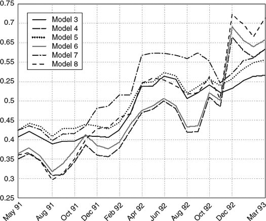
FIGURE 1.1 Time series estimates of Eastman Kodak Company's intensity function.

A typical time series graph of the default intensities for Eastman Kodak (ek) using models 3–8 is shown in Figure 1.1. As depicted, all six models exhibit similar patterns in the default intensities. The magnitude of the default intensity appears to be quite large, exceeding 0.3 for all dates and models.

Table 1.3 provides some summary statistics (both in- and out-of-sample) regarding the quality of the models fit to the data. Included are the average root mean squared error, the average generalized cross-validation statistic, the average default intensity, the average standard error of the default intensity, and the average 1-year default probability.

6. ANALYSIS OF THE TIME SERIES PROPERTIES OF THE PARAMETERS

Under the assumed model structure, the default and equity risk premium parameters λ_0t, λ_1t, λ_2t, β_0t, β_1t, β_2t, β_3t) should be constant across time. The 4-year estimation period was selected to better ensure this hypothesis, by minimizing the structural shifts in the economy that would more likely occur using a longer horizon interval. Given measurement error in the input data (equity prices and the state variable parameters) and its effect on the parameter estimates, we test the hypothesis that the time series variation in these parameters is solely due to random (white) noise. Alternatively stated, we test to see if the parameter estimates follow a random walk around a given mean. A unit root test is used in this regard.

Table 1.3 Summary Statistics for Model Performance

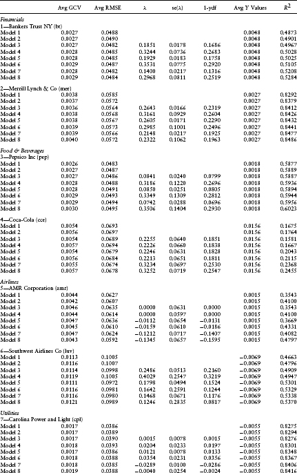
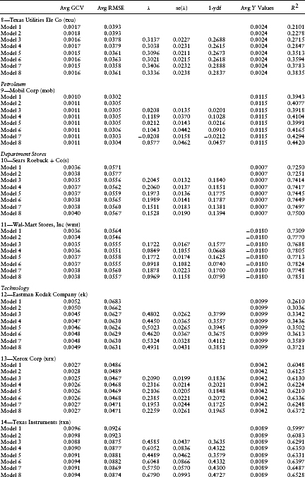
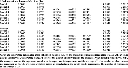
Table 1.4 Unit Root Test Performance across All Companies

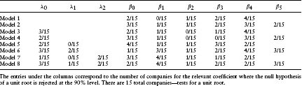
Table 1.4 contains a summary of the unit root rejections across model types. As seen, we accept a unit root (non-stationarity) for almost all the parameters in all the models. This includes both the default parameters and the risk premium coefficients. Acceptance of the unit root implies that the model parameters may be non-stationary. This non-stationarity could be due to a confounding of the default and risk premium parameter estimates. Given that the underlying variables related to both quantities are correlated, multicollinearity in the linear regression may be a problem.

7. ANALYSIS OF FAMA-FRENCH FOUR-FACTOR MODEL WITH NO DEFAULT

Before analyzing the default parameters, it is important to document the performance of the simple Fama–French four-factor model with no default. Table 1.2 contains the estimates for the coefficients of the Fama–French four-factor model with and without a P/E ratio (models 1 and 2, respectively) and their t-scores. The F-test for model 1 in Table 1.2 tests the hypothesis that the model is significant (i.e., β_0t = β_1t = β_2t = β_3t = β_4t = 0). For every firm, the average p-value for this F-test is 0.0000, strongly rejecting the hypothesis of no significance. This test confirms the need to include the Fama–French four-Factor model to explain stock risk premiums. The average R² for model 1 is 0.5018.

8. ANALYSIS OF A BUBBLE COMPONENT (P/E RATIO) IN STOCK PRICES

This section tests for the significance of a bubble component in equity returns by testing the null hypothesis that the P/E ratio is insignificant, that is, β_5t = 0. The F-test for model 2 in Table 1.2 also tests this hypothesis. For models 1 and 2 (not including default), the averages p-values for three firms (mer, amr, and ek) are significantly different from zero. The individual t-scores for β_5t show significance for four firms (mer, amr, wmt, and ek), confirming this conclusion. This represents 20% (=3/15) to 26% (=4/15) of our firms. For models 3–8 (including default), the average F-test gives significance for only one of these three firms (amr). The average t-scores for β_5t confirm this reduced significance. For amr alone (among the three: mer, amr, and ek), the estimated coefficient for the constant in the regression (λ₀) is zero.

It appears that for models with no default (models 1 and 2), the P/E ratio proxies for a bubble component in stock prices not contained in the four factors of Fama–French. But, for the models with default (models 3–8), the P/E ratio becomes insignificant. The inclusion of a constant in the regression model (λ₀) appears to confound the bubble component in stock 15 prices.¹⁵

An additional test for a possible model misspecification with respect to the bubble component is provided by the t-score for the stock's own variance (β₄). This t-score tests for the null hypothesis that β₄ = −1/2, the theoretical value as given in equation 1.6. As indicated, for all models and for all but four firms (cce, amr, mob, and ibm), one can reject the null hypothesis that β₄ = −1/2. This rejection is strong evidence consistent with the stock's own variance proxying for stock price bubbles.

In summary, this section provides evidence consistent with the existence of an equity price bubble not captured in the Fama–French four-factor model. Both the P/E ratio and the stock's own variance appear to be significant explanatory variables in the equity return regression model.

9. ANALYSIS OF THE DEFAULT INTENSITY

As mentioned earlier, the average default intensity parameters and t-scores are contained in Table 1.2. The firms' estimates are presented in industry groupings for easy comparison. First to be noticed is that the fit of the linear regressions is quite good. The average R² varies between 0.1581 (for cce, model 3) to 0.8486 (for mer, model 8). From Table 1.3, the average R² across all models varies from 0.5018 for model 1 to 0.5670 for model 8. R² uniformly increases across firms with increasing model complexity up to model 8. This is to be expected because R² is a measure of the in-sample fit, and as we progress from model 1 to model 8, more independent variables are added to the linear regression.

Second, it is interesting to examine the signs of the coefficients for the default intensity parameters. The signs of λ₁ and λ₂ indicate the sensitivity of the firm's default likelihood to changes in the spot rate and the cumulative excess return on the equity market index, respectively. For example, for wmt (Wal-Mart Stores) the sign of λ₁ is positive indicating that as interest rates rise, the likelihood of default increases. Continuing, the sign of λ₂ is negative, indicating that as the market index rises, the likelihood of default decreases. The signs of these coefficients differ across firms and between firms within an industry. An example of different signs within an industry is for the department stores grouping, where Sears Roebuck and Company (s) and Wal-Mart Stores, Inc. (wmt) have contrasting signs for both the interest rate and market index variables.

Next, we discuss the statistical significance of these point estimates. For λ₀, the point estimate is significantly different from zero in model 3 for seven firms (mer, txu, s, wmt, ek, xrx, txn, and ibm). The F-test for model 3 also tests the hypothesis that λ_0t = 0. This test confirms the average t-score results because the average p-scores are low (below 15% for five firms). Including the P/E ratio in model 4 eliminates the significance of the default parameter λ₀ for two of the seven firms (mer and wmt), indicating a possible confounding of the default parameter estimate with equity price bubbles. This suspicion is confirmed for more complex models 5–8. The pattern with respect to the significance of the default parameter λ₀ is similar to that previously discussed for models 3 and 4.

With respect to the spot rate coefficient, λ₁, the significance of its t-scores varies across firms and model types. For four out of the 15 firms, the average t-score is significantly different from zero for at least one of models 5–8. This observation is also supported by the F-test for model 5 (the joint hypothesis λ_0t = λ_1t = 0). The average p-scores for this F-test are less than 20% for five firms (luv, txu, ek, txn, and ibm). This evidence strongly supports the inclusion of the interest rate variable in the default intensity model.

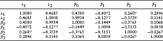
Finally, with respect to the market index coefficient, λ₂, the average t-scores indicate that it is insignificant from zero for all firms except one (amr). Unfortunately, the introduction of the independent variable (Z(t)(T_L – t) – Z(t – Δ)(T_L – (t – Δ))) into this regression causes a severe multicollinearity problem with another independent variable in the equity risk premium, the excess return on the market portfolio. As seen in models 7 and 8, for all firms the introduction of (Z(t)(T_L – t) – Z(t – Δ)(T_L – (t – Δ))) causes the point estimates of β₀ to change dramatically from their values in models 1–6 and β₀ becomes insignificantly different from zero. The correlation matrix in Table 1.5 confirms this multicollinearity problem. The correlation between these two variables is 0.9934. This implies that the estimates of the coefficients λ₂ and β₀ cannot be separated using this regression model. This evidence is consistent with a confounding of the default probability estimates with those of the equity's risk premium.

As seen from Table 1.3, the impact of these different default intensity models on the point estimates of the default intensities can be dramatic. For example, for mer the average default intensity varies from −0.0569 in model 7 to 0.3534 for model 6. Negative default intensities should be interpreted as being a point estimate of zero. Similar patterns can also be observed for the other firms in our sample. This sensitivity is consistent with a confounding of the default probability model with the equity risk premium and bubble component.

Table 1.5 Correlation Matrix for Selected Independent Variables in the Equity Model Regression

Also documented in Table 1.3 are the magnitudes of these default probability estimates. As indicated, they are quite high relative to historical default frequencies. Indeed, the average default intensity across all firms and all models exceeds 0.20, whereas the magnitude of the average historical default intensities observed from bankruptcy data is less than 0.01 (see Chava and Jarrow, 2002). Although this difference could be due to the fact that these estimates obtained are the risk-neutral probabilities, as opposed to the statistical probabilities, more likely the difference is due to a confounding of the default intensity model with both the equity risk premium and price bubble. As previously highlighted, many of the preceding test results are consistent with this second interpretation.

Also to be noticed at this juncture are the magnitudes of the RMSE of the regression model in comparison to the average magnitude of the dependent variable. The RMSE is an estimate of the standard error of the unpredictable component of equity returns. The average magnitude of the dependent variable is the average equity return over this period. As indicated in Table 1.3, the standard error of the unpredictable component of the equity's return is over 10 times the magnitude of its average value. This is true for all firms in our sample. This illustrates the magnitude of the “noise” in equity prices relative to our predictive ability using the Fama–French four-factor model. This noise inhibits our ability to estimate the default intensities with a great deal of precision.

In summary, an analysis of the default intensity parameters in the equity return regression model shows that although it is feasible to estimate the likelihood of default, the estimated intensity process parameters are confounded by the equity risk premium and price bubble component. Both default risk and the equity's risk premium appear to be positively correlated. Including both variables in a regression yields an upward bias in the estimated default probability (relative to historical default frequencies).

10. RELATIVE PERFORMANCE OF THE EQUITY RETURN MODELS

This section studies the relative performance of the eight equity return models. For each firm and for each model's regression, both a root mean squared error statistic (RMSE) and a generalized cross-validation statistic (GCV) are computed. The RMSE statistic measures the “average” pricing error between the model and the market price. It is an in-sample goodness-of-fit measure. As with all in-sample goodness of fit measures, a potential problem with RMSE is that it may provide a biased picture of the quality of model performance due to a model overfitting the noise in the data. The second GCV test statistic is designed to partially overcome this problem, as an out-of-sample goodness-of-fit measure that is predictive in nature.¹⁶ The lower the GCV statistic, the better the out-of-sample model fit.

The average RMSE and GCV statistics for each firm and model are contained in Table 1.6. For 13 of the 15 firms, the RMSE statistic is smallest (or within 0.0001 of the smallest value) for models 3–6. For all 15 firms, the GCV statistic is smallest (or within 0.0001 of the smallest value) for models 3–6. This is strong evidence consistent with the importance of including the default parameters into the equity return model and the feasibility of using equity returns to infer default intensity estimates.

Surprisingly, for no firms except one (txu) do models 7 and 8 have the smallest GCV statistics. Despite the multicollinearity problem present when including Z(t) into the default intensity process, this is strong evidence consistent with the insignificance of the λ₂ coefficient. This relative performance analysis confirms the insignificance of the λ₂ coefficient documented in Janosi et al. (2002) for the same firms, but using debt prices.

In summary, in terms of the GCV statistic, the best-fitting models are 3–6. Given the previous evidence with respect to the significance of the interest rate variable in the default intensity process, the preferred equity return models are probably 5 and 6.

11. COMPARISON OF DEFAULT INTENSITIES BASED ON DEBT VERSUS EQUITY

This section investigates the equality between the default intensities estimated using the equity returns with the default intensities as estimated in Janosi et al. (2002). Using the identical structure, the identical data, and the same time period as employed above, Janosi et al. (2002) estimate the expected loss per unit time λ(t)(1 – δ) implicit in debt prices, using a reduced-form credit risk model. Here, 0 ≤ δ ≤ 1 corresponds to the recovery rate on defaulted debt.

They selected 20 different firms, 15 of which overlap with this study (see Table 1.1). Janosi et al. (2002) estimated five different liquidity premium models. We use only the best-fitting model, the constant liquidity premium. To match the best-fitting equity pricing model (model 6), we use the intensity function from Janosi et al. (2002) without the market index included. For this credit risk model, we have the monthly time series of the estimated expected loss per unit time λ(t)(1 – δ) for each of the 15 companies from Janosi etal. (2002) and their standard errors. Unfortunately, due to nonoverlapping periods of observations in the two studies, only 10 firms are included in this comparison. The five firms omitted are: amr, bt, cce, cpl, and ek.

Table 1.6 Test for the Equivalence between the Default Intensities Based on Debt Prices versus Equity Prices

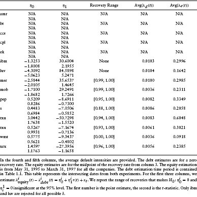
Available are estimated intensities λ_eⁱ(t) from the equity returns for firm i in month t, and estimated expected losses (per unit time) aⁱ_d(t) = λ_i^d(t)(1–δⁱ) from Janosi et al. (2002) for firm i in month t. The null hypothesis to be tested is

for all firms i and all months t.

Given an assumed value for the recovery rate δⁱ, we can do a pair-wise t-test (using the standard errors of the estimates) of the difference [aⁱ_d(t)/(1 – δⁱ)] – λⁱ_e(t) for a given firm i for each month t. Under the null hypothesis this difference is zero. Unfortunately, this is a joint test of the null hypothesis and the assumed value of δ_i. To eliminate this joint hypothesis, we test for equality of these differences over a range of different values for δⁱ from 0 to 1. If there is a value for δⁱ where the null hypothesis [ãⁱ_d(t)/(1 – δⁱ)] – λⁱ_e(t) = 0 is not rejected, then this value for δⁱ is an estimate of the recovery rate. The relevant summary statistics for these tests are contained in Table 1.6.

For all firms but two (ibm and luv), there is some recovery rate such that the two estimates can be viewed as equivalent. This is strong evidence consistent with equality of the implicit estimation procedures across both equity and debt prices. However, the recovery rate needed to obtain equality of the two estimates is in excess of 88%, for all firms except one (wmt). This recovery rate is higher than the average recovery rate of 67% contained in Moody's (1992) for senior secured debt over the time period 1974–1991. This overestimate of the recovery rate suggests an upward bias in the estimated default rates obtained from equity returns, confirming the conclusions from the previous analyses.

12. CONCLUSIONS

This chapter uses a reduced-form model to estimate default probabilities implicit in equity returns. The model implemented is a generalization of the model contained in Jarrow (2001). The time period covered is May 1991–March 1997. Monthly equity returns on 15 different firms are studied. The firms are chosen to provide a stratified sample across various industry groupings.

Three general conclusions can be drawn from this investigation. First, equity returns can be used to infer a firm's default intensities. This is a feasibility result. Second, equity returns appear to contain a bubble component, as proxied by the firm's P/E ratio. Bubbles in equity returns are not completely captured by the four-factor model of Fama and French (1993, 1996). Third, due to this imprecision in modeling equity risk premiums, the point estimates of the default intensities confound with the equity risk premium. Estimated default probabilities using equity returns are larger than those obtained based on either historical bankruptcy data or implicitly using debt prices. This conclusion casts doubts upon the reliability of the default probability estimates obtained from equity prices using structural models as in Delianedis and Geske (1998) (confirming the previous conclusions of Jarrow and van Deventer, 1998, 1999, and Jarrow et al., 2002, in this regard). This is also consistent with the inability of structural models using equity price information to explain credit spreads in corporate debt (see Collin-Dufresne et al., 2001; Huang and Huang, 2002; Eom et al., 2002).

NOTES

1. The intensity process is defined under the risk neutral probability.

2. This assumption is easily relaxed; see Jarrow (2001).

3. One could assume that these dividends could be defaulted on as well; see Jarrow (2001).

4. See Money Magazine April 1999, p. 169 for Yahoo's P/E ratio of 1176.6.

5. This is a simple no arbitrage restriction that the present value of the sum of multiple cash flows equals the sum of the present values of the cash flows.

6. For the explicit equations, see Jarrow (2001).

7. This is in contrast to the typical situation where there are multiple debt issues outstanding that can be utilized to implicitly estimate default intensities when using debt prices.

8. The appendix contains a minor correction to the formula contained in Jarrow (2001).

9. The address is: http://web.mit.edu/kfrenc/www/data_library.html.

10. We perform a Dickey–Fuller (DF) test. The DF test statistic is the t-statistic for the ρ coefficient in the regression y_t – y_t–1 = μ + ρy_t–1 + ε_t where μ, ρ are constants and ε_t is an error term. The null hypothesis of a unit root for y_t is ρ = 0. A rejection of the null hypothesis implies that there is no unit root. The unit root test statistics are σ_r(–2.6348) and a_r(–1.1632).

11. The unit root test statistics are σ_m (–3.9407) and φ(–1.3479).

12. The exact formula for this computation is in Jarrow (2001).

13. The t-score is adjusted to reflect the fact that the regressions contain overlapping time intervals; see Janosi et al. (2002) for more details on the adjustment.

14. This is not to be confused with the number of observations used in the time t regression for a particular firm. At the time t regression, we use 48 months of data.

15. This should not be surprising. In the standard implementation of the CAPM, the constant term in the regression equation is called the “alpha” and it is used to represent abnormal returns. If the bubble component is not adequately modeled, its time series variation would appear in the estimate of this coefficient.

16. Roughly speaking, the GCV statistics measure the average predictive error obtained by systematically eliminating each data point from the time series regression, predicting that point's value with the regression, and then measuring the “average” predictive error that results, after adjusting for degrees of freedom (see Wahba, 1985).

REFERENCES

Adams, K. and van Deventer, D. (1994). “Fitting Yield Curves and Forward Rate Curves with Maximum Smoothness.” Journal of Fixed Income June, 52–62.

Altman, E. I. (1968). “Financial Ratios, Discriminant Analysis and the Prediction of Corporate Bankruptcy.” Journal of Finance 23, 589–609.

Bielecki, T. and Rutkowski, M. (2000). Credit Risk: Modelling, Valuation and Hedging. New York: Springer-Verlag (in press).

Chava, S. and Jarrow, R. (2002). “Bankruptcy Prediction with Industry Effects.” Working paper, Cornell University.

Collin-Dufresne, P., Goldstein, R. and Martin, J. (2001). “The Determinants of Credit Spread Changes.” Journal of Finance 54, 2177–2207.

Delianedis, G. and Geske, R. (1998). “Credit Risk and Risk Neutral Default Probabilities: Information about Rating Migrations and Defaults.” Working paper, UCLA.

Dimson, E. (1979), “Risk Measurement when Shares are Subject to Infrequent Trading.” Journal of Financial Economics 7, 197–226.

Duffee, G. (1999). “Estimating the Price of Default Risk.” The Review of Financial Studies 12, 197–226.

Duffie, D. and Singleton, K. (1997). “An Econometric Model of the Term Structure of Interest Rate Swap Yields.” Journal of Finance 52, 1287–1321.

Duffie, D. and Singleton, K. (1999). “Modeling Term Structures of Defaultable Bonds.” Review of Financial Studies 12, 197–226.

Duffie, D., Pedersen, L. and Singleton, K. (2000). “Modeling Sovereign Yield Spreads: A Case Study of Russian Debt.” Working paper, Stanford University.

Eom, Y., Helwege, J. and Huang, J. (2002). “Structural Models of Corporate Bond Pricing: An Empirical Analysis.” Working paper, Penn State University.

Fama, E. and French, K. (1993). “Common Risk Factors in the Returns on Stocks and Bonds.” Journal of Financial Economics 33, 3–56.

Fama, E. and French, K. (1996). “Multifactor Explanations of Asset Pricing Anomalies.” Journal of Finance 60, 55–84.

Heath, D., Jarrow, R. and Morton, A. (1992). “Bond Pricing and the Term Structure of Interest Rates: A New Methodology for Contingent Claim Valuation.” Econometrica 60, 77–105.

Huang, J. and Huang, M. (2002). “How Much of the Corporate Treasury Yield Spread Is Due to Credit Risk.” Working paper, Penn State University.

Hull, J. and White, A. (2000). “Valuing Credit Default Swaps I: No Counterparty Default Risk.” Journal of Derivatives 8, 29–40.

Hull, J. and White, A. (2001). “Valuing Credit Default Swaps II: Modeling Default Correlations.” Journal of Derivatives 8, 12–23.

Janosi, T. and Jarrow, R. (2002). “Maximum Smoothness Forward Rate Curves.” Working paper, Cornell University.

Janosi, T., Jarrow, R. and Yildirim, Y. (2002). “Estimating Expected Losses and Liquidity Discounts Implicit in Debt Prices.” Journal of Risk 5, 1–39.

Jarrow, R. (2001). “Default Parameter Estimation Using Market Prices.” Financial Analysts Journal 57, 75–92.

Jarrow, R. and van Deventer, D. (1998). “Integrating Interest Rate Risk and Credit Risk in Asset and Liability Management.” Asset and Liability Management: The Synthesis of New Methodologies. Risk Publications.

Jarrow, R. and van Deventer, D. (1999). “Practical Usage of Credit Risk Models in Loan Portfolio and Counterparty Exposure Management.” Credit Risk Models and Management. Risk Publications.

Jarrow, R. and Madan, D. (2000). “Arbitrage, Martingales and Private Monetary Value.” Journal of Risk 3, 73–90.

Madan, D. and Unal, H. (1998). “Pricing the Risks of Default.” Review of Derivatives Research 2, 121–160.

Moody's Special Report (1992). Corporate Bond Defaults and Default Rates. New York: Moody's Investors Service.

Risk Magazine (2000). “Credit Risk: A Risk Special Report.” (March).

Schwartz, R. and Whitcomb, D. (1977a). “The Time-Variance Relationship: Evidence on Autocorrelation in Common Stock Returns.” Journal of Finance 32, 41–55.

Schwartz, R. and Whitcomb, D. (1977b). “Evidence on the Presence and Causes of Serial Correlation in Market Model Residuals.” Journal of Financial and Quantitative Analysis June, 291–313.

Shumway, T. (2001). “Forecasting Bankruptcy More Accurately: A Simple Hazard Model.” Journal of Business (in press).

Smith, K. (1978). “The Effect of Intervaling on Estimating Parameters of the Capital Asset Pricing Model.” Journal of Financial and Quantitative Analysis June, 313–332.

Warga, A. (1999). Fixed Income Data Base. University of Houston, College of Business Administration (www.uh.edu/~awarga/lb.html).

Wahba, G. (1985). “A Comparison of GCV and GLM for Choosing the Smoothing Parameter in the Generalized Spline Smoothing Problem.” Annals of Statistics 13, 1378–1402.

Zmijewski, M.E. (1984). “Methodological Issues Related to the Estimation of Financial Distress Prediction Models.” Journal of Accounting Research 22,59–82.

APPENDIX

From the appendix in Jarrow (2001), we have:

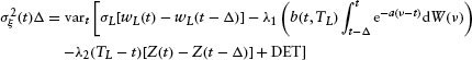
In the previous expression, the following quantities are unobservable: φ_rL, φ_mL. To eliminate these quantities from this expression, we compute the variance of the preceding expression.

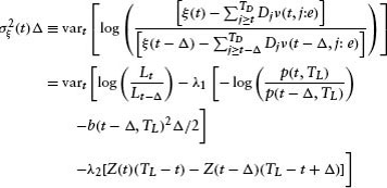
But we have:

where DET indicates nonrandom terms. Also note that

Substitution gives

Combined, we get:

Computing this variance yields:

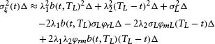
where we have used the facts:

and

Rearranging the terms gives:

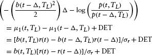
Substitution gives the result:

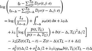
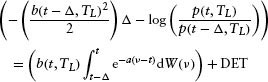
Using Girsanov's theorem, we have the original Brownian motion: w_L(t) = (t) + ∫₀^t Θ_L(u) du where (t) is a Brownian motion under the statistical measure and Θ_L(u) is the liquidation value's risk premium. Hence,

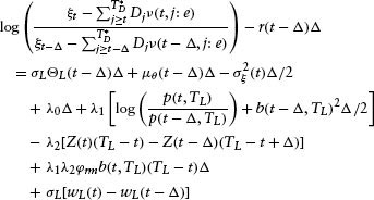
Thus, we have the final result:

---

^aComputer Science Department, Cornell University, Ithaca, NY, USA.

^bJohnson Graduate School of Management, Cornell University, Ithaca, NY, and Kamakura Corporation, USA.

^cSchool of Management, Syracuse University, Syracuse, NY, USA.

^*Corresponding author. Johnson Graduate School of Management, Cornell University, Ithaca, NY 14853, USA. Tel.: +1 607 255 4729; e-mail: [email protected].