Appendix B—Big O Notation

Big O notation, also known as asymptotic notation, is a way of summarizing the performance of algorithms based on problem size. The problem size is usually designated n. The “Big O”-ness of an algorithm is often referred to as its complexity. The term asymptotic is used as it describes the behavior of a function as its input size approaches infinity.

As an example, consider an unsorted array that contains a value we need to search for. Because it is unsorted, we will have to search every element until we find the value we are looking for. If the array is of size n, we will need to search, worst case, n elements. We say, therefore, that this linear search algorithm has a complexity of O(n).

That is the worst case. On average, however, the algorithm will need to look at n / 2 elements, so we could be more accurate and say the algorithm is, on average, O(n / 2), but this is not actually a significant change as far as the growth factor (n) is concerned, so constants are dropped, leaving us with the same O(n) complexity.

Big O notation is expressed in terms of functions of n, where n is the problem size, which is determined by the algorithm and the data structure it operates on. For a collection, it could be the number of items in the collection; for a string search algorithm, it is the length of the respective strings.

Big O notation is concerned with how the time required to perform an algorithm grows with ever larger input sizes. With our array example, we expect that if the array were to double in length, then the time required to search the array would also double. This implies that the algorithm has linear performance characteristics.

An algorithm with complexity of O(n²) would exhibit worse than linear performance. If the input doubles, the time is quadrupled. If problem size increases by a factor of 8, then the time increases by a factor of 64, always squared. This type of algorithm exhibits quadratic complexity. A good example of this is the bubble sort algorithm (in fact, most naïve sorting algorithms have O(n²) complexity).

private static void BubbleSort(int[] array)
{
bool swapped;
do
{
swapped = false;
for (int i = 1; i < array.Length; i++)
{
if (array[i - 1] > array[i])
{
int temp = array[i - 1];
array[i - 1] = array[i];
array[i] = temp;
swapped = true;
}
}
} while (swapped);
}

Any time you see nested loops, it is quite likely the algorithm is going to be quadratic or polynomial (if not worse). In bubble sort’s case, the outer loop can run up to n times while the inner loop examines up to n elements on each iteration. O(n * n) == O(n²).

When analyzing your own algorithms, you may come up with a formula that contains multiple factors, as in O(8n² + n + C) (a quadratic portion multiplied by 8, a linear portion, and a constant time portion). For the purposes of Big O notation, only the most significant factor is kept and multiplicative constants are ignored. This algorithm would be regarded as O(n²). Remember, too, that Big O notation is concerned with the growth of the time as the problem size approaches infinity. Even though 8n² is 8 times larger than n², it is not very relevant compared to the growth of the n² factor, which far outstrips every other factor for large values of n. If n is small, the difference between O(n log n), O(n²), or O(2ⁿ) is trivial and uninteresting.

Many algorithms have multiple inputs and their complexity can be denoted with both variables, e.g., O(mn) or O(m+n). Many graph algorithms, for example, depend on the number of edges and the number of vertices.

The most common types of complexity are:

• O(1)—Constant—The time required does not depend on size of the input. Many hash tables have O(1) complexity.
• O(log n)—Logarithmic—Time increases as a fraction of the input size. Any algorithm that cuts its problems space in half on each iteration exhibits logarithmic complexity. Note that there is no specific number base for this log.
• O(n)—Linear—Time increases linearly with input size.
• O(n log n)—Loglinear—Time increases quasilinearly, that is, the time is dominated by a linear factor, but this is multiplied by a fraction of the input size.
• O(n²)—Quadratic—Time increases with the square of the input size.
• O(n^c) —Polynomial—C is greater than 2.
• O(cⁿ) —Exponential—C is greater than 1.
• O(n!)—Factorial—Basically, try every possibility.

Algorithmic complexity is usually described in terms of its average and worst-case performance. Best-case performance is not very interesting because, for many algorithms, luck can be involved (e.g., it does not really matter for our analysis that the best-case performance of linear search is O(1) because that means it just happened to get lucky).

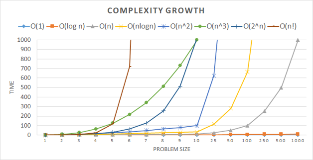
The following graph shows how fast time can grow based on problem size. Note that the difference between O(1) and O(log n) is almost indistinguishable even out to relatively large problem sizes. An algorithm with O(n!) complexity is almost unusable with anything but the smallest problem sizes.

Though time is the most common dimension of complexity, space (memory usage) can also be analyzed with the same methodology.

1. Common Algorithms and Their Complexity

Sorting

• Quicksort—O(n log n), O(n²) worst case
• Merge sort—O(n log n)
• Heap sort—O(n log n)
• Bubble sort—O(n²)
• Insertion sort—O(n²)
• Selection sort—O(n²)

Graphs

• Depth-first search—O(E + V) (E = Edges, V = Vertices)
• Breadth-first search—O(E + V)
• Shortest-path (using Min-heap)—O((E + V) log V)

Searching

• Unsorted array—O(n)
• Sorted array with binary search—O(log n)
• Binary search tree—O(log n)
• Hash table—O(1)

Special case

• Traveling salesman—O(n!)

Often, O(n!) is really just shorthand for “brute force, try every possibility.”