Chapter 3. Recommending Music and the Audioscrobbler Data Set
The recommender engine is one of the most popular example of large-scale machine learning, and most people have seen Amazon’s. It is a common denominator because recommender engines are everywhere, from social networks to video sites to online retailers. We can also directly observe them in action. We’re aware that a computer is picking tracks to play on Spotify, in much the same way we don’t necessarily notice that Gmail is deciding whether inbound email is spam.
The output of a recommender is more intuitively understandable than other machine learning algorithms. It’s exciting, even. For as much as we think that musical taste is personal and inexplicable, recommenders do a surprisingly good job of identifying tracks we didn’t know we would like. For domains like music or movies where recommenders are usually deployed, it’s comparatively easy to reason about why a recommended piece of music fits with someone’s listening history. Not all clustering or classification algorithms match that description. For example, a support vector machine classifier is a set of coefficients, and it’s hard even for practitioners to articulate what the numbers mean when they make predictions.
It seems fitting to kick off the next three chapters, which will explore key machine learning algorithms on PySpark, with a chapter built around recommender engines, and recommending music in particular. It’s an accessible way to introduce real-world use of PySpark and MLlib, and some basic machine learning ideas that will be developed in subsequent chapters.
In this chapter, we will implement a recommender system in PySpark. Specifically, we will use the Alternating Least Squares (ALS) algorithm on an open dataset provided by a music streaming service. We will start off by understanding the dataset and importing it in PySpark. We will then discuss our motivation for choosing the ALS algorithm and its implementation in PySpark. This will be followed by data preparation and building our model using PySpark. We will finish off by making some user recommendations and discussing ways to improve our model through hyperparameter selection.
Setting up the Data
We will will use a data set published by Audioscrobbler. Audioscrobbler was the first music recommendation system for last.fm, one of the first internet streaming radio sites, founded in 2002. Audioscrobbler provided an open API for “scrobbling,” or recording listeners’ song plays. last.fm used this information to build a powerful music recommender engine. The system reached millions of users because third-party apps and sites could provide listening data back to the recommender engine.
At that time, research on recommender engines was mostly confined to learning from rating-like data. That is, recommenders were usually viewed as tools that operated on input like “Bob rates Prince 3.5 stars.” The Audioscrobbler data set is interesting because it merely records plays: “Bob played a Prince track.” A play carries less information than a rating. Just because Bob played the track doesn’t mean he actually liked it. You or I may occasionally play a song by an artist we don’t care for, or even play an album and walk out of the room.
However, listeners rate music far less frequently than they play music. A data set like this is therefore much larger, covers more users and artists, and contains more total information than a rating data set, even if each individual data point carries less information. This type of data is often called implicit feedback data because the user-artist connections are implied as a side effect of other actions, and not given as explicit ratings or thumbs-up.
A snapshot of a data set distributed by last.fm in 2005 can be found online as a compressed archive. Download the archive, and find within it several files. First, the data set’s files need to be made available. If you are using a remote cluster, copy all three data files into HDFS. This chapter will assume that the files are available at /user/ds/.
Start pyspark-shell. Note that the computations in this chapter will take up more memory than simple applications. If you are running locally rather than on a cluster, for example, you will likely need to specify something like --driver-memory 4g to have enough memory to complete these computations. The main data set is in the user_artist_data.txt file. It contains about 141,000 unique users, and 1.6 million unique artists. About 24.2 million users’ plays of artists are recorded, along with their counts. Let’s read this data set into a DataFrame and have a look at it.
raw_user_artist_data=spark.read.text("user/ds/user_artist_data.txt")raw_user_artist_data.show(5)...+-------------------+|value|+-------------------+|1000002155||1000002100000633||100000210000078||10000021000009144||10000021000010314|+-------------------+
By default on HDFS, the data set will contain one partition for each HDFS block. Because this file consumes about 400 MB on disk, it will split into about three to six partitions given typical HDFS block sizes. Machine learning tasks like ALS are likely to be more compute-intensive than simple text processing. It may be better to break the data into smaller pieces—more partitions—for processing. You can chain a call to .repartition(n) after reading the text file to specify a different and larger number of partitions. You might set this higher to match the number of cores in your cluster, for example.
The data set also gives the names of each artist by ID in the artist_data.txt file. Note that when plays are scrobbled, the client application submits the name of the artist being played. This name could be misspelled or nonstandard, and this may only be detected later. For example, “The Smiths,” “Smiths, The,” and “the smiths” may appear as distinct artist IDs in the data set even though they are plainly the same. So, the data set also includes artist_alias.txt, which maps artist IDs that are known misspellings or variants to the canonical ID of that artist. Let’s read in these two data sets into PySpark too.
raw_artist_data=spark.read.text("user/ds/artist_data.txt")raw_artist_data.show(5)...+--------------------+|value|+--------------------+|113499906CrazyLife||6821360PangNakarin||10113088Terfel,...||10151459TheFlam...||6826647Bodenstan...|+--------------------+...raw_artist_alias=spark.read.text("user/ds/artist_alias.txt")raw_artist_alias.show(5)...+----------------+|value|+----------------+|10927641000311||10951221000557||67080701007267||100880541042317||11959171042317|+----------------+
We now have a basic understanding of the datasets. We will now discuss our requirements from a recommender algorithm and subsequently understand why the Alternating Least Squares algorithm is a good choice.
Our requirements from a recommender system
We need to choose a recommender algorithm that is suitable for our data. Here are our considerations:
-
Implicit feedback.
It is comprised entirely of interactions between users and artists’ songs. It contains no information about the users, or about the artists other than their names. We need an algorithm that learns without access to user or artist attributes. These are typically called collaborative filtering algorithms. For example, deciding that two users might share similar tastes because they are the same age is not an example of collaborative filtering. Deciding that two users might both like the same song because they play many other same songs is an example.
-
Sparsity
Our data set looks large because it contains tens of millions of play counts. But in a different sense, it is small and skimpy, because it is sparse. On average, each user has played songs from about 171 artists—out of 1.6 million. Some users have listened to only one artist. We need an algorithm that can provide decent recommendations to even these users. After all, every single listener must have started with just one play at some point!
-
Scalability and real-time predictions
Finally, we need an algorithm that scales, both in its ability to build large models and to create recommendations quickly. Recommendations are typically required in near real time—within a second, not tomorrow.
A broad class of algorithms that may be suitable are latent-factor models. They try to explain observed interactions between large numbers of users and items through a relatively small number of unobserved, underlying reasons. For example, consider a customer who has bought albums by metal bands Megadeth and Pantera, but also classical composer Mozart. It may be difficult to explain why exactly these albums were bought and nothing else. However, it’s probably a small window on a much larger set of tastes. Maybe the customer likes a coherent spectrum of music from metal to progressive rock to classical. That explanation is simpler, and as a bonus, suggests many other albums that would be of interest. In this example, “liking metal, progressive rock, and classical” are three latent factors that could explain tens of thousands of individual album preferences.
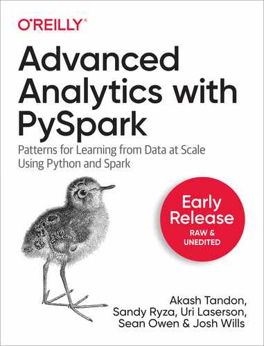
In our case, we will specifically use a type of matrix factorization model. Mathematically, these algorithms treat the user and product data as if it were a large matrix A, where the entry at row i and column j exists if user i has played artist j. A is sparse: most entries of A are 0, because only a few of all possible user-artist combinations actually appear in the data. They factor A as the matrix product of two smaller matrices, X and Y. They are very skinny—both have many rows because A has many rows and columns, but both have just a few columns (k). The k columns correspond to the latent factors that are being used to explain the interaction data.
The factorization can only be approximate because k is small, as shown in Figure 3-1.
Figure 3-1. Matrix factorization
These algorithms are sometimes called matrix completion algorithms, because the original matrix A may be quite sparse, but the product XYT is dense. Very few, if any, entries are 0, and therefore the model is only an approximation to A. It is a model in the sense that it produces (“completes”) a value for even the many entries that are missing (that is, 0) in the original A.
This is a case where, happily, the linear algebra maps directly and elegantly to intuition. These two matrices contain a row for each user and each artist, respectively. The rows have few values—k. Each value corresponds to a latent feature in the model. So the rows express how much users and artists associate with these k latent features, which might correspond to tastes or genres. And it is simply the product of a user-feature and feature-artist matrix that yields a complete estimation of the entire, dense user-artist interaction matrix. This product might be thought of as mapping items to their attributes, and then weighting those by user attributes.
The bad news is that A = XYT generally has no exact solution at all, because X and Y aren’t large enough (technically speaking, too low rank) to perfectly represent A. This is actually a good thing. A is just a tiny sample of all interactions that could happen. In a way, we believe A is a terribly spotty and therefore hard-to-explain view of a simpler underlying reality that is well explained by just some small number of factors, k, of them. Think of a jigsaw puzzle depicting a cat. The final puzzle is simple to describe: a cat. When you’re holding just a few pieces, however, the picture you see is quite difficult to describe.
XYT should still be as close to A as possible. After all, it’s all we’ve got to go on. It will not and should not reproduce it exactly. The bad news again is that this can’t be solved directly for both the best X and best Y at the same time. The good news is that it’s trivial to solve for the best X if Y is known, and vice versa. But neither is known beforehand!
Fortunately, there are algorithms that can escape this catch-22 and find a decent solution. One such algorithm that’s available in PySpark is the ALS algorithm.
Alternating Least Squares algorithm
We will use the Alternating Least Squares (ALS) algorithm to compute latent factors from our dataset. This type of approach was popularized around the time of the Netflix Prize by papers like “Collaborative Filtering for Implicit Feedback Datasets” and “Large-Scale Parallel Collaborative Filtering for the Netflix Prize”. PySpark MLlib’s ALS implementation draws on ideas from both of these papers and is the only recommender algorithm currently implemented in Spark MLlib.
Here’s a code snippet (non-functional) to give you a peek at what lies ahead in the chapter.
frompyspark.ml.recommendationimportALSals=ALS(maxIter=5,regParam=0.01,userCol="user",itemCol="artist",ratingCol="count")model=als.fit(train)predictions=model.transform(test)
With ALS, we will treat our input data as a large sparse matrix A, and find out X and Y, as discussed in previous section. At the start, Y isn’t known, but it can be initialized to a matrix full of randomly chosen row vectors. Then simple linear algebra gives the best solution for X, given A and Y. In fact, it’s trivial to compute each row i of X separately as a function of Y and of one row of A. Because it can be done separately, it can be done in parallel, and that is an excellent property for large-scale computation:
AiY(YTY)–1 = Xi
Equality can’t be achieved exactly, so in fact the goal is to minimize |AiY(YTY)–1 – Xi|, or the sum of squared differences between the two matrices’ entries. This is where the “least squares” in the name comes from. In practice, this is never solved by actually computing inverses but faster and more directly via methods like the QR decomposition. This equation simply elaborates on the theory of how the row vector is computed.
The same thing can be done to compute each Yj from X. And again, to compute X from Y, and so on. This is where the “alternating” part comes from. There’s just one small problem: Y was made up, and random! X was computed optimally, yes, but given a bogus solution for Y. Fortunately, if this process is repeated, X and Y do eventually converge to decent solutions.
When used to factor a matrix representing implicit data, there is a little more complexity to the ALS factorization. It is not factoring the input matrix A directly, but a matrix P of 0s and 1s, containing 1 where A contains a positive value and 0 elsewhere. The values in A are incorporated later as weights. This detail is beyond the scope of this book, but is not necessary to understand how to use the algorithm.
Finally, the ALS algorithm can take advantage of the sparsity of the input data as well. This, and its reliance on simple, optimized linear algebra and its data-parallel nature, make it very fast at large scale.
Next, we will preprocess our dataset and make it suitable for use with the ALS algorithm.
Preparing the Data
The first step in building a model is to understand the data that is available, and parse or transform it into forms that are useful for analysis in Spark.
Spark MLlib’s ALS implementation does not strictly require numeric IDs for users and items, but is more efficient when the IDs are in fact representable as 32-bit integers. It’s advantageous to use Int to represent IDs, but this would mean that the IDs can’t exceed Int.MaxValue, or 2147483647. Does this data set conform to this requirement already?
raw_user_artist_data.show(10)...+-------------------+|value|+-------------------+|1000002155||1000002100000633||100000210000078||10000021000009144||10000021000010314||100000210000138||1000002100001442||1000002100001769||10000021000024329||100000210000251|+-------------------+
Each line of the file contains a user ID, an artist ID, and a play count, separated by spaces. To compute statistics on the user ID, we split the line by space characters, and parse the values as integers. The result is conceptually three “columns”: a user ID, artist ID and count as Ints. It makes sense to transform this to a data frame with columns named “user”, “artist”, and “count” because it then becomes simple to compute simple statistics like the maximum and minimum:
frompyspark.sql.functionsimportsplit,min,maxfrompyspark.sql.typesimportIntegerType,StringTypeuser_artist_df=raw_user_artist_data.withColumn('user',split(raw_user_artist_data['value'],' ').getItem(0).cast(IntegerType())).withColumn('artist',split(raw_user_artist_data['value'],' ').getItem(1).cast(IntegerType())).withColumn('count',split(raw_user_artist_data['value'],' ').getItem(2).cast(IntegerType())).drop('value')user_artist_df.select([min("user"),max("user"),min("artist"),max("artist")]).show()...+---------+---------+-----------+-----------+|min(user)|max(user)|min(artist)|max(artist)|+---------+---------+-----------+-----------+|90|2443548|1|10794401|+---------+---------+-----------+-----------+
The maximum user and artist IDs are 2443548 and 10794401, respectively (and their minimums are 90 and 1; no negative values). These are comfortably smaller than 2147483647. No additional transformation will be necessary to use these IDs.
It will be useful later in this example to know the artist names corresponding to the opaque numeric IDs. raw_artist_data contains the artist ID and name separated by a tab. PySpark’s split function accepts regular expression values for the pattern parameter. We can split using the whitespace character, s:
frompyspark.sql.functionsimportcolartist_by_id=raw_artist_data.withColumn('id',split(col('value'),'s+',2).getItem(0).cast(IntegerType())).withColumn('name',split(col('value'),'s+',2).getItem(1).cast(StringType())).drop('value')artist_by_id.show(5)...+--------+--------------------+|id|name|+--------+--------------------+|1134999|06CrazyLife||6821360|PangNakarin||10113088|Terfel,Bartoli-...||10151459|TheFlamingSidebur||6826647|Bodenstandig3000|+--------+--------------------+
This gives a data frame with the artist ID and name as columns “id” and “name”.
raw_artist_alias maps artist IDs that may be misspelled or nonstandard to the ID of the artist’s canonical name. This dataset is relatively small, containing about 200,000 entries. It contains two IDs per line, separated by a tab. We will parse this in a similar manner as we did raw_artist_data.
artist_alias=raw_artist_alias.withColumn('artist',split(col('value'),'s+').getItem(0).cast(IntegerType())).withColumn('alias',split(col('value'),'s+').getItem(1).cast(StringType())).drop('value')artist_alias.show(5)...+--------+-------+|artist|alias|+--------+-------+|1092764|1000311||1095122|1000557||6708070|1007267||10088054|1042317||1195917|1042317|+--------+-------+
The first entry maps ID 1092764 to 1000311. We can look these up from artist_by_id DataFrame:
artist_by_id.filter(artist_by_id.id.isin(1092764,1000311)).show()...+-------+--------------+|id|name|+-------+--------------+|1000311|SteveWinwood||1092764|Winwood,Steve|+-------+--------------+
This entry evidently maps “Winwood, Steve” to “Steve Winwood,” which is in fact the correct name for the artist.
Building a First Model
Although the data set is in nearly the right form for use with Spark MLlib’s ALS implementation, it requires a small extra transformation. The aliases data set should be applied to convert all artist IDs to a canonical ID, if a different canonical ID exists.
frompyspark.sql.functionsimportbroadcast,whentrain_data=train_data=user_artist_df.join(broadcast(artist_alias),'artist',how='left').withColumn('artist',when(col('alias').isNull(),col('artist')).otherwise(col('alias'))).withColumn('artist',col('artist').cast(IntegerType())).drop('alias')train_data.cache()

Get artist’s alias if it exists, otherwise get original artist.
We broadcast the artist_alias DataFrame created earlier.. This makes Spark send and hold in memory just one copy for each executor in the cluster. When there are thousands tasks and many execute
in parallel on each executor, this can save significant network traffic and memory. As a rule of thumb, its helpful to broadcast a significantly smaller dataset when performing a join with a very big dataset.
The call to cache() suggests to Spark that this DataFrame should be temporarily stored after being computed, and furthermore, kept in memory in the cluster. This is helpful because the ALS algorithm is iterative, and will typically need to access this data 10 times or more. Without this, the DataFrame could be repeatedly recomputed from the original data each time it is accessed! The Storage tab in the Spark UI will show how much of the DataFrame is cached and how much memory it uses, as shown in Figure 3-2. This one consumes about 120 MB across the cluster.
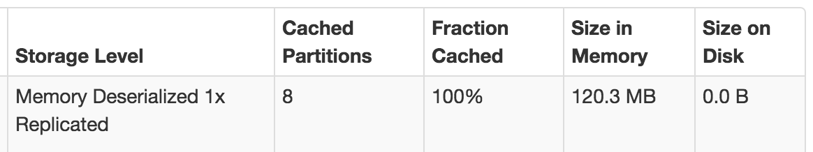
Figure 3-2. Storage tab in the Spark UI, showing cached DataFrame memory usage
Note that the label “Deserialized” in the UI above is actually only relevant for RDDs, where “Serialized” means data are stored in memory not as objects, but as serialized bytes. However, DataFrame instances like this one perform their own “encoding” of common data types in memory separately.
Actually, 120 MB is surprisingly small. Given that there are about 24 million plays stored here, a quick back-of-the-envelope calculation suggests that this would mean that each user-artist-count entry consumes only 5 bytes on average. However, the three 32-bit integers alone ought to consume 12 bytes. This is one of the advantages of a DataFrame. Because the types of data stored are primitive 32-bit integers, their representation can be optimized in memory internally.
Finally, we can build a model:
frompyspark.ml.recommendationimportALSmodel=ALS(rank=10,seed=0,maxIter=5,regParam=0.1,implicitPrefs=True,alpha=1.0,userCol='user',itemCol='artist',ratingCol='count').fit(train_data)
This constructs model as an ALSModel with some default configuration. The operation will likely take minutes or more depending on your cluster. Compared to some machine learning models, whose final form may consist of just a few parameters or coefficients, this type of model is huge. It contains a feature vector of 10 values for each user and product in the model, and in this case there are more than 1.7 million of them. The model contains these large user-feature and product-feature matrices as DataFrames of their own.
The values in your results may be somewhat different. The final model depends on a randomly chosen
initial set of feature vectors. The default behavior of this and other components in MLlib, however, is to use the same set of random choices every time by defaulting to a fixed seed. This is unlike other libraries, where behavior of random elements is typically not fixed by default. So, here and elsewhere, a random seed is set with (… seed=0,…).
To see some feature vectors, try the following, which displays just one row and does not truncate the wide display of the feature vector:
model.userFactors.show(1,truncate=False)...+---+-----------------------------------------------...|id|features...+---+-----------------------------------------------...|90|[0.16020626,0.20717518,-0.1719469,0.06038466...+---+-----------------------------------------------...
The other methods invoked on ALS, like setAlpha, set hyperparameters whose value can affect the quality of the recommendations that the model makes. These will be explained later. The more important first question is, is the model any good? Does it produce good recommendations? That is what we will try to answer in the next section.
Spot Checking Recommendations
We should first see if the artist recommendations make any intuitive sense, by examining a user, plays, and recommendations for that user. Take, for example, user 2093760. First, let’s look at his or her plays to get a sense of the person’s tastes. Extract the IDs of artists that this user has listened to and print their names. This means searching the input for artist IDs played by this user, and then filtering the set of artists by these IDs in order to print the names in order:
user_id=2093760existing_artist_ids=train_data.filter(train_data.user==user_id).select("artist").collect()existing_artist_ids=[i[0]foriinexisting_artist_ids]artist_by_id.filter(col('id').isin(existing_artist_ids)).show()...+-------+---------------+|id|name|+-------+---------------+|1180|DavidGray||378|Blackalicious||813|Jurassic5||1255340|TheSawDoctors||942|Xzibit|+-------+---------------+
Find lines whose user is 2093760.

Collect data set of artist ID.

Filter in those artists.
The artists look like a mix of mainstream pop and hip-hop. A Jurassic 5 fan? Remember, it’s 2005. In case you’re wondering, the Saw Doctors are a very Irish rock band popular in Ireland.
Now, it’s simple to make recommendations for a user, though computing them this way will take a few moments. It’s suitable for batch scoring but not real-time use cases:
user_subset=train_data.select('user').where(col('user')==user_id).distinct()top_predictions=model.recommendForUserSubset(user_subset,5)top_predictions.show()...+-------+--------------------+|user|recommendations|+-------+--------------------+|2093760|[[2814,0.0294106...|+-------+--------------------+
The resulting recommendations contain lists comprised of artist ID and of course, “predictions.” For this type of ALS algorithm, the prediction is an opaque value normally between 0 and 1, where higher values mean a better recommendation. It is not a probability, but can be thought of as an estimate of a 0/1 value indicating whether the user won’t or will interact with the artist, respectively.
After extracting the artist IDs for the recommendations, we can look up artist names in a similar way:
top_predictions_pandas=top_predictions.toPandas()(top_prediction_pandas)...userrecommendations02093760[(2814,0.029410675168037415),(1300642,0.028......recommended_artist_ids=[i[0]foriintop_predictions_pandas.recommendations[0]]artist_by_id.filter(col('id').isin(recommended_artist_ids)).show()...+-------+----------+|id|name|+-------+----------+|2814|50Cent||4605|SnoopDogg||1007614|Jay-Z||1001819|2Pac||1300642|TheGame|+-------+----------+
The result is all hip-hop. This doesn’t look like a great set of recommendations, at first glance. While these are generally popular artists, they don’t appear to be personalized to this user’s listening habits.
Evaluating Recommendation Quality
Of course, that’s just one subjective judgment about one user’s results. It’s hard for anyone but that user to quantify how good the recommendations are. Moreover, it’s infeasible to have any human manually score even a small sample of the output to evaluate the results.
It’s reasonable to assume that users tend to play songs from artists who are appealing, and not play songs from artists who aren’t appealing. So, the plays for a user give a partial picture of “good” and “bad” artist recommendations. This is a problematic assumption but about the best that can be done without any other data. For example, presumably user 2093760 likes many more artists than the 5 listed previously, and among the 1.7 million other artists not played, a few are of interest and not all are “bad” recommendations.
What if a recommender were evaluated on its ability to rank good artists high in a list of recommendations? This is one of several generic metrics that can be applied to a system that ranks things, like a recommender. The problem is that “good” is defined as “artists the user has listened to,” and the recommender system has already received all of this information as input. It could trivially return the user’s previously listened-to artists as top recommendations and score perfectly. But this is not useful, especially because the recommender’s role is to recommend artists that the user has never listened to.
To make this meaningful, some of the artist play data can be set aside and hidden from the ALS model-building process. Then, this held-out data can be interpreted as a collection of good recommendations for each user but one that the recommender has not already been given. The recommender is asked to rank all items in the model, and the ranks of the held-out artists are examined. Ideally, the recommender places all of them at or near the top of the list.
We can then compute the recommender’s score by comparing all held-out artists’ ranks to the rest. (In practice, we compute this by examining only a sample of all such pairs, because a potentially huge number of such pairs may exist.) The fraction of pairs where the held-out artist is ranked higher is its score. A score of 1.0 is perfect, 0.0 is the worst possible score, and 0.5 is the expected value achieved from randomly ranking artists.
This metric is directly related to an information retrieval concept called the receiver operating characteristic (ROC) curve. The metric in the preceding paragraph equals the area under this ROC curve, and is indeed known as AUC, or Area Under the Curve. AUC may be viewed as the probability that a randomly chosen good recommendation ranks above a randomly chosen bad recommendation.
The AUC metric is also used in the evaluation of classifiers. It is implemented, along with related
methods, in the MLlib class BinaryClassificationMetrics. For recommenders, we will compute AUC
per user and average the result. The resulting metric is slightly different, and might be
called “mean AUC.” We will implement this, because it is not (quite) implemented in PySpark.
Other evaluation metrics that are relevant to systems that rank things are implemented in
RankingMetrics. These include metrics like precision, recall, and mean average precision (MAP). MAP is also frequently used and focuses more narrowly on the quality of the top recommendations. However, AUC will be used here as a common and broad measure of the quality of the entire model output.
In fact, the process of holding out some data to select a model and evaluate its accuracy is common practice in all of machine learning. Typically, data is divided into three subsets: training, cross-validation (CV), and test sets. For simplicity in this initial example, only two sets will be used: training and CV. This will be sufficient to choose a model. In Chapter 4, this idea will be extended to include the test set.
Computing AUC
An implementation of mean AUC is provided in the source code accompanying this book. It is not reproduced here, but is explained in some detail in comments in the source code. It accepts the CV set as the “positive” or “good” artists for each user, and a prediction function. This function translates a data frame containing each user-artist pair into a data frame that also contains its estimated strength of interaction as a “prediction,” a number wherein higher values mean higher rank in the recommendations.
In order to use it, we must split the input data into a training and CV set. The ALS model will be trained on the training data set only, and the CV set will be used to evaluate the model. Here, 90% of the data is used for training and the remaining 10% for cross-validation:
defareaUnderCurve(positive_data,b_all_artist_IDs,predict_function):...valallData=buildCounts(rawUserArtistData,bArtistAlias)valArray(trainData,cvData)=allData.randomSplit(Array(0.9,0.1))trainData.cache()cvData.cache()valallArtistIDs=allData.select("artist").as[Int].distinct().collect()valbAllArtistIDs=spark.sparkContext.broadcast(allArtistIDs)valmodel=newALS().setSeed(Random.nextLong()).setImplicitPrefs(true).setRank(10).setRegParam(0.01).setAlpha(1.0).setMaxIter(5).setUserCol("user").setItemCol("artist").setRatingCol("count").setPredictionCol("prediction").fit(trainData)areaUnderCurve(cvData,bAllArtistIDs,model.transform)
Note that this function is defined above.
Remove duplicates, and collect to driver.
Note that areaUnderCurve() accepts a function as its third argument. Here, the transform method from
ALSModel is passed in, but it will shortly be swapped out for an alternative.
The result is about 0.879. Is this good? It is certainly higher than the 0.5 that is expected from making recommendations randomly, and it’s close to 1.0, which is the maximum possible score. Generally, an AUC over 0.9 would be considered high.
But is it an accurate evaluation? This evaluation could be repeated with a different 90% as the training set. The resulting AUC values’ average might be a better estimate of the algorithm’s performance on the data set. In fact, one common practice is to divide the data into k subsets of similar size, use k – 1 subsets together for training, and evaluate on the remaining subset. We can repeat this k times, using a different set of subsets each time. This is called k-fold cross-validation. This won’t be implemented in examples here, for simplicity, but some support for this technique exists in MLlib in its CrossValidator API. The validation API will be revisited in [Link to Come].
It’s helpful to benchmark this against a simpler approach. For example, consider recommending the globally most-played artists to every user. This is not personalized, but it is simple and may be effective. Define this simple prediction function and evaluate its AUC score:
defpredictMostListened(train:DataFrame)(allData:DataFrame)={vallistenCounts=train.groupBy("artist").agg(sum("count").as("prediction")).select("artist","prediction")allData.join(listenCounts,Seq("artist"),"left_outer").select("user","artist","prediction")}areaUnderCurve(cvData,bAllArtistIDs,predictMostListened(trainData))
This is another interesting demonstration of Scala syntax, where the function appears to be defined to take
two lists of arguments. Calling the function and supplying the first argument creates a
partially applied function, which itself takes an argument (allData) in order to return predictions.
The result of predictMostListened(trainData) is a function.
The result is also about 0.880. This suggests that nonpersonalized recommendations are already fairly effective according to this metric. However, we’d expect the “personalized” recommendations to score better in comparison. Clearly, the model needs some tuning. Can it be made better?
Hyperparameter Selection
So far, the hyperparameter values used to build the ALSModel were simply given without comment.
They are not learned by the algorithm and must be chosen by the caller. The configured hyperparameters were:
setRank(10)-
The number of latent factors in the model, or equivalently, the number of columns k in the user-feature and product-feature matrices. In nontrivial cases, this is also their rank.
setMaxIter(5)-
The number of iterations that the factorization runs. More iterations take more time but may produce a better factorization.
setRegParam(0.01)-
A standard overfitting parameter, also usually called lambda. Higher values resist overfitting, but values that are too high hurt the factorization’s accuracy.
setAlpha(1.0)-
Controls the relative weight of observed versus unobserved user-product interactions in the factorization.
rank, regParam, and alpha can be considered hyperparameters to the model.
(maxIter is more of a constraint on resources used in the factorization.) These are not values that end up in the matrices inside the ALSModel—those are simply its parameters and are chosen by the algorithm. These hyperparameters are instead parameters to the process of building itself.
The values used in the preceding list are not necessarily optimal. Choosing good hyperparameter values is a common problem in machine learning. The most basic way to choose values is to simply try combinations of values and evaluate a metric for each of them, and choose the combination that produces the best value of the metric.
In the following example, eight possible combinations are tried: rank = 5 or 30, regParam = 4.0 or 0.0001, and alpha = 1.0 or 40.0. These values are still something of a guess, but are chosen to cover a broad range of parameter values. The results are printed in order by top AUC score:
valevaluations=for(rank<-Seq(5,30);regParam<-Seq(4.0,0.0001);alpha<-Seq(1.0,40.0))yield{valmodel=newALS().setSeed(Random.nextLong()).setImplicitPrefs(true).setRank(rank).setRegParam(regParam).setAlpha(alpha).setMaxIter(20).setUserCol("user").setItemCol("artist").setRatingCol("count").setPredictionCol("prediction").fit(trainData)valauc=areaUnderCurve(cvData,bAllArtistIDs,model.transform)model.userFactors.unpersist()model.itemFactors.unpersist()(auc,(rank,regParam,alpha))}evaluations.sorted.reverse.foreach(println)...(0.8928367485129145,(30,4.0,40.0))(0.891835487024326,(30,1.0E-4,40.0))(0.8912376926662007,(30,4.0,1.0))(0.889240668173946,(5,4.0,40.0))(0.8886268430389741,(5,4.0,1.0))(0.8883278461068959,(5,1.0E-4,40.0))(0.8825350012228627,(5,1.0E-4,1.0))(0.8770527940660278,(30,1.0E-4,1.0))
Read as a triply nested
forloop.Free up model resources immediately.
Sort by first value (AUC), descending, and print.
The for syntax here is a way to write nested loops in Scala. It is like a loop over alpha, inside a loop over regParam, inside a loop over rank.
The differences are small in absolute terms, but are still
somewhat significant for AUC values. Interestingly, the parameter alpha seems consistently better at 40 than 1. (For the curious,
40 was a value proposed as a default in one of the original ALS papers mentioned earlier.) This can be interpreted
as indicating that the model is better off focusing far more on what the user did listen to
than what he or she did not listen to.
A higher regParam looks better too. This suggests the model is somewhat susceptible to overfitting,
and so needs a higher regParam to resist trying to fit the sparse input given from each user too exactly.
Overfitting will be revisited in more detail in [Link to Come].
As expected, 5 features is pretty low for a model of this size, and underperforms the model that uses 30 features to explain tastes. It’s possible that the best number of features is actually higher than 30, and that these values are alike in being too small.
Of course, this process can be repeated for different ranges of values or more values. It is a brute-force means of choosing hyperparameters. However, in a world where clusters with terabytes of memory and hundreds of cores are not uncommon, and with frameworks like Spark that can exploit parallelism and memory for speed, it becomes quite feasible.
It is not strictly required to understand what the hyperparameters mean, although it is helpful to know what normal ranges of values are like in order to start the search over a parameter space that is neither too large nor too tiny.
This was a fairly manual way to loop over hyperparameters, build models, and evaluate them.
In Chapter 4, after learning more about the Spark ML API, we’ll find that
there is a more automated way to compute this using Pipelines and TrainValidationSplit.
Making Recommendations
Proceeding for the moment with the best set of hyperparameters, what does the new model recommend for user 2093760?
+-----------+
|       name|
+-----------+
|  [unknown]|
|The Beatles|
|     Eminem|
|         U2|
|  Green Day|
+-----------+
Anecdotally, this makes a bit more sense for this user, being dominated by pop rock instead of all hip-hop. [unknown] is plainly not an artist. Querying the original data set reveals that it occurs 429,447 times, putting it nearly in the top 100! This is some default value for plays without an artist, maybe supplied by a certain scrobbling client. It is not useful information and we should discard it from the input before starting again. It is an example of how the practice of data science is often iterative, with discoveries about the data occurring at every stage.
This model can be used to make recommendations for all users. This could be useful in a batch process that recomputes a model and recommendations for users every hour or even less, depending on the size of the data and speed of the cluster.
At the moment, however, Spark MLlib’s ALS implementation does not support a method to recommend to all users. It is possible to recommend to one user at a time, as shown above, although each will launch a short-lived distributed job that takes a few seconds. This may be suitable for rapidly recomputing recommendations for small groups of users. Here, recommendations are made to 100 users taken from the data and printed:
valsomeUsers=allData.select("user").as[Int].distinct().take(100)valsomeRecommendations=someUsers.map(userID=>(userID,makeRecommendations(model,userID,5)))someRecommendations.foreach{case(userID,recsDF)=>valrecommendedArtists=recsDF.select("artist").as[Int].collect()println(s"$userID -> ${recommendedArtists.mkString(",")}")}...1000190->6694932,435,1005820,58,12443621001043->1854,4267,1006016,4468,12741001129->234,1411,1307,189,121...
Copy 100 (distinct) users to the driver.
map()is a local Scala operation here.mkStringjoins a collection to a string with a delimiter.
Here, the recommendations are just printed. They could just as easily be written to an external store like HBase, which provides fast lookup at runtime.
Interestingly, this entire process could also be used to recommend users to artists. This could be used to answer questions like “Which 100 users are most likely to be interested in the new album by artist X?” Doing so would only require swapping the user and artist field when parsing the input:
rawArtistData.map{line=>val(id,name)=line.span(_!='')(name.trim,id.int)}
Where to Go from Here
Naturally, it’s possible to spend more time tuning the model parameters, and finding and fixing anomalies in the input, like the [unknown] artist. For example, a quick analysis of play counts reveals that user
2064012 played artist 4468 an astonishing 439,771 times! Artist 4468 is the implausibly successful alterna-metal band System of a Down,
who turned up earlier in recommendations. Assuming an average song length of 4 minutes, this is over 33 years of playing hits like “Chop Suey!” and “B.Y.O.B.” Because the band started making records in 1998, this would require playing four or five tracks at once for seven years. It must be spam or a data error, and another example of the types of real-world data problems that a production system would have to address.
ALS is not the only possible recommender algorithm, but at this time, it is the only one supported by
Spark MLlib. However, MLlib also supports a variant of ALS for non-implicit data. Its use is identical,
except that ALS is configured with setImplicitPrefs(false). This is appropriate when data is rating-like,
rather than count-like. For example, it is appropriate when the data set is user ratings of artists on a 1–5 scale.
The resulting prediction column returned from ALSModel.transform recommendation methods then really is
an estimated rating. In this case, the simple RMSE (root mean squared error) metric is appropriate for
evaluating the recommender.
Later, other recommender algorithms may be available in Spark MLlib or other libraries.
In production, recommender engines often need to make recommendations in real time, because they are used in contexts like ecommerce sites where recommendations are requested frequently as customers browse product pages. Precomputing and storing recommendations in a NoSQL store, as mentioned previously, is a reasonable way to make recommendations available at scale. One disadvantage of this approach is that it requires precomputing recommendations for all users who might need recommendations soon, which is potentially any of them. For example, if only 10,000 of 1 million users visit a site in a day, precomputing all million users’ recommendations each day is 99% wasted effort.
It would be nicer to compute recommendations on the fly, as needed. While we can compute recommendations for one user using the ALSModel, this is necessarily a distributed operation that takes several seconds, because ALSModel is uniquely large and therefore actually a distributed data set. This is not true of other models, which afford much faster scoring. Projects like Oryx 2 attempt to implement real-time on-demand recommendations with libraries like MLlib by efficiently accessing the model data in memory.