
4
Sorting and Searching
There are a few workhorse algorithms we use in nearly every kind of program. Sometimes these algorithms are so fundamental that we take them for granted or don’t even realize our code is relying on them.
Several methods for sorting and searching are among these fundamental algorithms. They’re worth knowing because they’re commonly used and beloved by algorithm enthusiasts (and the sadists who give coding interviews). The implementation of these algorithms can be short and simple, but every character matters, and since they are so commonly needed, computer scientists have striven to enable them to sort and search with mind-melting speed. So we’ll also use this chapter to discuss algorithm speed and the special notation we use to compare algorithms’ efficiencies.
We start by introducing insertion sort, a simple and intuitive sorting algorithm. We discuss the speed and efficiency of insertion sort and how to measure algorithm efficiency in general. Next, we look at merge sort, a faster algorithm that is the current state of the art for searching. We also explore sleep sort, a strange algorithm that isn’t used much in practice but is interesting as a curiosity. Finally, we discuss binary search and show some interesting applications of searching, including inverting mathematical functions.
Insertion Sort
Imagine that you’ve been asked to sort all the files in a filing cabinet. Each file has a number assigned to it, and you need to rearrange the files so that the file with the lowest number is first in the cabinet, the file with the highest number is last, and the files’ numbers proceed in order in between.
Whatever method you follow as you sort the filing cabinet, we can describe it as a “sorting algorithm.” But before you even think of opening Python to code an algorithm for this, take a moment to pause and consider how you would sort such a filing cabinet in real life. This may seem like a mundane task, but allow the adventurer within you to creatively consider a broad range of possibilities.
In this section, we present a very simple sorting algorithm called insertion sort. This method relies on looking at each item in a list one at a time and inserting it into a new list that ends up being correctly sorted. Our algorithm’s code will have two sections: an insertion section, which performs the humble task of inserting a file into a list, and a sorting section, which performs insertion repeatedly until we have completed our sorting task.
Putting the Insertion in Insertion Sort
First, consider the task of insertion itself. Imagine that you have a filing cabinet whose files are already perfectly sorted. If someone hands you one new file and asks you to insert it into the right (sorted) position in the filing cabinet, how do you accomplish that? The task may seem so simple that it doesn’t warrant an explanation, or even the possibility of one (just do it! you might think). But in the world of algorithms, every task, however humble, must be explained completely.
The following method describes a reasonable algorithm for inserting one file into a sorted filing cabinet. We’ll call the file we need to insert the “file to insert.” We’ll say that we can compare two files and call one file “higher than” the other one. This could mean that one file’s assigned number is higher than the other’s assigned number, or it could mean that it’s higher in an alphabetical or other ordering.
- Select the highest file in the filing cabinet. (We’ll start at the back of the cabinet and work our way to the front.)
- Compare the file you have selected with the file to insert.
- If the file you have selected is lower than the file to insert, place the file to insert one position behind that file.
- If the file you have selected is higher than the file to insert, select the next highest file in the filing cabinet.
- Repeat steps 2 to 4 until you have inserted your file or compared it with every existing file. If you have not yet inserted your file after comparing it with every existing file, insert it at the beginning of the filing cabinet.
That method should more or less match the intuition you have for how to insert a record into a sorted list. If you prefer, you could also start at the beginning of the list, instead of the end, and follow an analogous process with the same results. Notice that we haven’t just inserted a record; we’ve inserted a record in the correct position, so after insertion, we’ll still have a sorted list. We can write a script in Python that executes this insertion algorithm. First, we can define our sorted filing cabinet. In this case, our filing cabinet will be a Python list, and our files will simply be numbers.
cabinet = [1,2,3,3,4,6,8,12]Then, we can define the “file” (in this case, just a number) that we want to insert into our cabinet.
to_insert = 5We proceed one at a time through every number in the list (every file in the cabinet). We’ll define a variable called check_location. As advertised, it will store the location in the cabinet that we want to check. We start at the back of the cabinet:
check_location = len(cabinet) - 1We’ll also define a variable called insert_location. The goal of our algorithm is to determine the proper value of insert_location, and then it’s a simple matter of inserting the file at the insert_location. We’ll start out by assuming the insert_location is 0:
insert_location = 0Then we can use a simple if statement to check whether the file to insert is higher than the file at the check_location. As soon as we encounter a number that’s lower than the number to insert, we use its location to decide where to insert our new number. We add 1 because our insertion takes place just behind the lower number we found:
if to_insert > cabinet[check_location]:
    insert_location = check_location + 1
After we know the right insert_location, we can use a built-in Python method for list manipulation called insert to put the file into the cabinet:
cabinet.insert(insert_location,to_insert)Running this code will not work to insert our file properly yet, however. We need to put these steps together in one coherent insertion function. This function combines all of the previous code and also adds a while loop. The while loop is used to iterate over the files in the cabinet, starting with the last file and proceeding until either we find the right insert_location or we have examined every file. The final code for our cabinet insertion is in Listing 4-1.
def insert_cabinet(cabinet,to_insert):
  check_location = len(cabinet) - 1
  insert_location = 0
  while(check_location >= 0):
    if to_insert > cabinet[check_location]:
        insert_location = check_location + 1
        check_location = - 1
    check_location = check_location - 1
  cabinet.insert(insert_location,to_insert)
  return(cabinet)

cabinet = [1,2,3,3,4,6,8,12]
newcabinet = insert_cabinet(cabinet,5)
print(newcabinet)
Listing 4-1: Inserting a numbered file into our cabinet
When you run the code in Listing 4-1, it will print out newcabinet, which you can see includes our new “file,” 5, inserted into our cabinet at the correct location (between 4 and 6).
It’s worthwhile to think for a moment about one edge case of insertion: inserting into an empty list. Our insertion algorithm mentioned “proceeding sequentially through every file in the filing cabinet.” If there are no files in the filing cabinet, then there is nothing to proceed through sequentially. In this case, we need to heed only the last sentence, which tells us to insert our new file at the beginning of the cabinet. Of course, this is easier done than said, because the beginning of an empty cabinet is also the end and the middle of the cabinet. So all we need to do in this case is insert the file into the cabinet without regard to position. We can do this by using the insert() function in Python and inserting at location 0.
Sorting via Insertion
Now that we’ve rigorously defined insertion and know how to perform it, we’re almost at the point where we can perform an insertion sort. Insertion sort is simple: it takes each element of an unsorted list one at a time and uses our insertion algorithm to insert it correctly into a new, sorted list. In filing cabinet terms, we start with an unsorted filing cabinet, which we’ll call “old cabinet,” and an empty cabinet, which we’ll call “new cabinet.” We remove the first element of our old unsorted cabinet and add it to our new empty cabinet, using the insertion algorithm. We do the same with the second element of the old cabinet, then the third, and so on until we have inserted every element of the old cabinet into the new cabinet. Then, we forget about the old cabinet and use only our new, sorted cabinet. Since we’ve been inserting using our insertion algorithm, and it always returns a sorted list, we know that our new cabinet will be sorted at the end of the process.
In Python, we start with an unsorted cabinet and an empty newcabinet:
cabinet = [8,4,6,1,2,5,3,7]
newcabinet = []
We implement insertion sort by repeatedly calling our insert_cabinet() function from Listing 4-1. In order to call it, we’ll need to have a file in our “hand,” which we accomplish by popping it out of the unsorted cabinet:
to_insert = cabinet.pop(0)
newcabinet = insert_cabinet(newcabinet, to_insert)
In this snippet, we used a method called pop(). This method removes a list element at a specified index. In this case, we removed the element of cabinet at index 0. After we use pop(), cabinet no longer contains that element, and we store it in the variable to_insert so that we can put it into the newcabinet.
We’ll put all of this together in Listing 4-2, where we define an insertion_sort() function that loops through every element of our unsorted cabinet, inserting the elements one by one into newcabinet. Finally, at the end, we print out the result, a sorted cabinet called sortedcabinet.
cabinet = [8,4,6,1,2,5,3,7]
def insertion_sort(cabinet):
  newcabinet = []
  while len(cabinet) > 0:
    to_insert = cabinet.pop(0)
    newcabinet = insert_cabinet(newcabinet, to_insert)
  return(newcabinet)

sortedcabinet = insertion_sort(cabinet)
print(sortedcabinet)
Listing 4-2: An implementation of insertion sort
Now that we can do insertion sort, we can sort any list we encounter. We may be tempted to think that this means we have all the sorting knowledge we’ll ever need. However, sorting is so fundamental and important that we want to be able to do it in the best possible way. Before we discuss alternatives to insertion sort, let’s look at what it means for one algorithm to be better than another and, on an even more basic level, what it means for an algorithm to be good.
Measuring Algorithm Efficiency
Is insertion sort a good algorithm? This question is hard to answer unless we’re sure about what we mean by “good.” Insertion sort works—it sorts lists—so it’s good in the sense that it accomplishes its purpose. Another point in its favor is that it’s easy to understand and explain with reference to physical tasks that many people are familiar with. Yet another feather in its cap is that it doesn’t take too many lines of code to express. So far, insertion sort seems like a good algorithm.
However, insertion sort has one crucial failing: it takes a long time to perform. The code in Listing 4-2 almost certainly ran in less than one second on your computer, so the “long time” that insertion sort takes is not the long time that it takes for a tiny seed to become a mighty redwood or even the long time that it takes to wait in line at the DMV. It’s more like a long time in comparison to how long it takes a gnat to flap its wings once.
To fret about a gnat’s wing flap as a “long time” may seem a little extreme. But there are several good reasons to push algorithms as close as possible to zero-second running times.
Why Aim for Efficiency?
The first reason to relentlessly pursue algorithm efficiency is that it can increase our raw capabilities. If your inefficient algorithm takes one minute to sort an eight-item list, that may not seem like a problem. But consider that such an inefficient algorithm might take an hour to sort a thousand-item list, and a week to sort a million-item list. It may take a year or a century to sort a billion-item list, or it may not be able to sort it at all. If we make the algorithm better able to sort an eight-item list (something that seems trivial since it saves us only a minute), it may make the difference between being able to sort a billion-item list in an hour rather than a century, which can open up many possibilities. Advanced machine-learning methods like k-means clustering and k-NN supervised learning rely on ordering long lists, and improving the performance of a fundamental algorithm like sorting can enable us to perform these methods on big datasets that would otherwise be beyond our grasp.
Even sorting short lists is important to do quickly if it’s something that we have to do many times. The world’s search engines, for example, collectively receive a trillion searches every few months and have to order each set of results from most to least relevant before delivering them to users. If they can cut the time required for one simple sort from one second to half a second, they cut their required processing time from a trillion seconds to half a trillion seconds. This saves time for users (saving a thousand seconds for half a billion people really adds up!) and reduces data processing costs, and by consuming less energy, efficient algorithms are even environmentally friendly.
The final reason to create faster algorithms is the same reason that people try to do better in any pursuit. Even though there is no obvious need for it, people try to run the 100-meter dash faster, play chess better, and cook a tastier pizza than anyone ever has before. They do these things for the same reason George Mallory said he wanted to climb Mount Everest: “because it’s there.” It’s human nature to push the boundaries of the possible and strive to be better, faster, stronger, and more intelligent than anyone else. Algorithm researchers are trying to do better because, among other reasons, they wish to do something remarkable, whether or not it is practically useful.
Measuring Time Precisely
Since the time required for an algorithm to run is so important, we should be more precise than saying that insertion sort takes a “long time” or “less than a second.” How long, exactly, does it take? For a literal answer, we can use the timeit module in Python. With timeit, we can create a timer that we start just before running our sorting code and end just afterward. When we check the difference between the starting time and the ending time, we find how long it took to run our code.
from timeit import default_timer as timer

start = timer()
cabinet = [8,4,6,1,2,5,3,7]
sortedcabinet = insertion_sort(cabinet)
end = timer()
print(end - start)
When I ran this code on my consumer-grade laptop, it ran in about 0.0017 seconds. This is a reasonable way to express how good insertion sort is—it can fully sort a list with eight items in 0.0017 seconds. If we want to compare insertion sort with any other sorting algorithm, we can compare the results of this timeit timing to see which is faster, and say the faster one is better.
However, using these timings to compare algorithm performance has some problems. For example, when I ran the timing code a second time on my laptop, I found that it ran in 0.0008 seconds. A third time, I found that it ran on another computer in 0.03 seconds. The precise timing you get depends on the speed and architecture of your hardware, the current load on your operating system (OS), the version of Python you’re running, the OS’s internal task schedulers, the efficiency of your code, and probably other chaotic vagaries of randomness and electron motion and the phases of the moon. Since we can get very different results in each timing attempt, it’s hard to rely on timings to communicate about algorithms’ comparative efficiency. One programmer may brag that they can sort a list in Y seconds, while another programmer laughs and says that their algorithm gets better performance in Z seconds. We might find out they are running exactly the same code, but on different hardware at different times, so their comparison is not of algorithm efficiency but rather of hardware speed and luck.
Counting Steps
Instead of using timings in seconds, a more reliable measure of algorithm performance is the number of steps required to execute the algorithm. The number of steps an algorithm takes is a feature of the algorithm itself and isn’t dependent on the hardware architecture or even necessarily on the programming language. Listing 4-3 is our insertion sort code from Listings 4-1 and 4-2 with several lines added where we have specified stepcounter+=1. We increase our step counter every time we pick up a new file to insert from the old cabinet, every time we compare that file to another file in the new cabinet, and every time we insert the file into the new cabinet.
def insert_cabinet(cabinet,to_insert):
  check_location = len(cabinet) - 1
  insert_location = 0
  global stepcounter
  while(check_location >= 0):
    stepcounter += 1
    if to_insert > cabinet[check_location]:
        insert_location = check_location + 1
        check_location = - 1
    check_location = check_location - 1
  stepcounter += 1
  cabinet.insert(insert_location,to_insert)
  return(cabinet)

def insertion_sort(cabinet):
  newcabinet = []
  global stepcounter
  while len(cabinet) > 0:
    stepcounter += 1
    to_insert = cabinet.pop(0)
    newcabinet = insert_cabinet(newcabinet,to_insert)
  return(newcabinet)

cabinet = [8,4,6,1,2,5,3,7]
stepcounter = 0
sortedcabinet = insertion_sort(cabinet)
print(stepcounter)
Listing 4-3: Our insertion sort code with a step counter
In this case, we can run this code and see that it performs 36 steps in order to accomplish the insertion sort for a list of length 8. Let’s try to perform insertion sort for lists of other lengths and see how many steps we take.
To do so, let’s write a function that can check the number of steps required for insertion sort for unsorted lists of different lengths. Instead of manually writing out each unsorted list, we can use a simple list comprehension in Python to generate a random list of any specified length. We can import Python’s random module to make the random creation of lists easier. Here’s how we can create a random unsorted cabinet of length 10:
import random
size_of_cabinet = 10
cabinet = [int(1000 * random.random()) for i in range(size_of_cabinet)]
Our function will simply generate a list of some given length, run our insertion sort code, and return the final value it finds for stepcounter.
def check_steps(size_of_cabinet):
  cabinet = [int(1000 * random.random()) for i in range(size_of_cabinet)]
  global stepcounter
  stepcounter = 0
  sortedcabinet = insertion_sort(cabinet)
  return(stepcounter)
Let’s create a list of all numbers between 1 and 100 and check the number of steps required to sort lists of each length.
random.seed(5040)
xs = list(range(1,100))
ys = [check_steps(x) for x in xs]
print(ys)
In this code, we start by calling the random.seed() function. This is not necessary but will ensure that you see the same results as those printed here if you run the same code. You can see that we define sets of values for x, stored in xs, and a set of values for y, stored in ys. The x values are simply the numbers between 1 and 100, and the y values are the number of steps required to sort randomly generated lists of each size corresponding to each x. If you look at the output, you can see how many steps insertion sort took to sort randomly generated lists of lengths 1, 2, 3 . . . , all the way to 99. We can plot the relationship between list length and sorting steps as follows. We’ll import matplotlib.pyplot in order to accomplish the plotting.
import matplotlib.pyplot as plt
plt.plot(xs,ys)
plt.title('Steps Required for Insertion Sort for Random Cabinets')
plt.xlabel('Number of Files in Random Cabinet')
plt.ylabel('Steps Required to Sort Cabinet by Insertion Sort')
plt.show()
Figure 4-1 shows the output. You can see that the output curve is a little jagged—sometimes a longer list will be sorted in fewer steps than will a shorter list. The reason for this is that we generated every list randomly. Occasionally our random list generation code will create a list that’s easy for insertion sort to deal with quickly (because it’s already partially sorted), and occasionally it will create a list that is harder to deal with quickly, strictly through random chance. For this same reason, you may find that the output on your screen doesn’t look exactly like the output printed here if you don’t use the same random seed, but the general shape should be the same.

Figure 4-1: Insertion sort steps
Comparing to Well-Known Functions
Looking beyond the superficial jaggedness of Figure 4-1, we can examine the general shape of the curve and try to reason about its growth rate. The number of steps required appears to grow quite slowly between x = 1 and about x = 10. After that, it seems to slowly get steeper (and more jagged). Between about x = 90 and x = 100, the growth rate appears very steep indeed.
Saying that the plot gets gradually steeper as the list length increases is still not as precise as we want to be. Sometimes we talk colloquially about this kind of accelerating growth as “exponential.” Are we dealing with exponential growth here? Strictly speaking, there is a function called the exponential function defined by ex, where e is Euler’s number, or about 2.71828. So does the number of steps required for insertion sort follow this exponential function that we could say fits the narrowest possible definition of exponential growth? We can get a clue about the answer by plotting our step curve together with an exponential growth curve, as follows. We will also import the numpy module in order to take the maximum and minimum of our step values.
import math
import numpy as np
random.seed(5040)
xs = list(range(1,100))
ys = [check_steps(x) for x in xs]
ys_exp = [math.exp(x) for x in xs]
plt.plot(xs,ys)
axes = plt.gca()
axes.set_ylim([np.min(ys),np.max(ys) + 140])
plt.plot(xs,ys_exp)
plt.title('Comparing Insertion Sort to the Exponential Function')
plt.xlabel('Number of Files in Random Cabinet')
plt.ylabel('Steps Required to Sort Cabinet')
plt.show()
Just like before, we define xs to be all the numbers between 1 and 100, and ys to be the number of steps required to sort randomly generated lists of each size corresponding to each x. We also define a variable called ys_exp, which is ex for each of the values stored in xs. We then plot both ys and ys_exp on the same plot. The result enables us to see how the growth of the number of steps required to sort a list relates to true exponential growth.
Running this code creates the plot shown in Figure 4-2.
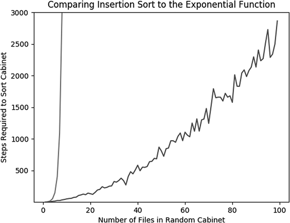
Figure 4-2: Insertion sort steps compared to the exponential function
We can see the true exponential growth curve shooting up toward infinity on the left side of the plot. Though the insertion sort step curve grows at an accelerating rate, its acceleration does not seem to get close to matching true exponential growth. If you plot other curves whose growth rate could also be called exponential, 2× or 10×, you’ll see that all of these types of curves also grow much faster than our insertion sort step counter curve does. So if the insertion sort step curve doesn’t match exponential growth, what kind of growth might it match? Let’s try to plot a few more functions on the same plot. Here, we’ll plot y = x, y = x1.5, y = x2, and y = x3 along with the insertion sort step curve.
random.seed(5040)
xs = list(range(1,100))
ys = [check_steps(x) for x in xs]
xs_exp = [math.exp(x) for x in xs]
xs_squared = [x**2 for x in xs]
xs_threehalves = [x**1.5 for x in xs]
xs_cubed = [x**3 for x in xs]
plt.plot(xs,ys)
axes = plt.gca()
axes.set_ylim([np.min(ys),np.max(ys) + 140])
plt.plot(xs,xs_exp)
plt.plot(xs,xs)
plt.plot(xs,xs_squared)
plt.plot(xs,xs_cubed)
plt.plot(xs,xs_threehalves)
plt.title('Comparing Insertion Sort to Other Growth Rates')
plt.xlabel('Number of Files in Random Cabinet')
plt.ylabel('Steps Required to Sort Cabinet')
plt.show()
This results in Figure 4-3.

Figure 4-3: Insertion sort steps compared to other growth rates
There are five growth rates plotted in Figure 4-3, in addition to the jagged curve counting the steps required for insertion sort. You can see that the exponential curve grows the fastest, and next to it the cubic curve scarcely even makes an appearance on the plot because it also grows so fast. The y = x curve grows extremely slowly compared to the other curves; you can see it at the very bottom of the plot.
The curves that are the closest to the insertion sort curve are y = x2 and y = x1.5. It isn’t obvious which curve is most comparable to the insertion sort curve, so we cannot speak with certainty about the exact growth rate of insertion sort. But after plotting, we’re able to make a statement like “if we are sorting a list with n elements, insertion sort will take somewhere between n1.5 and n2 steps.” This is a more precise and robust statement than “as long as a gnat’s wing flap” or “.002-ish seconds on my unique laptop this morning.”
Adding Even More Theoretical Precision
To get even more precise, we should try to reason carefully about the steps required for insertion sort. Let’s imagine, once again, that we have a new unsorted list with n elements. In Table 4-2, we proceed through each step of insertion sort individually and count the steps.
Table 4-2: Counting the Steps in Insertion Sort
| Description of actions | Number of steps required for pulling the file from the old cabinet | Maximum number of steps required for comparing to other files | Number of steps required for inserting the file into the new cabinet |
| Take the first file from the old cabinet and insert it into the (empty) new cabinet. | 1 | 0. (There are no files to compare to.) | 1 |
| Take the second file from the old cabinet and insert it into the new cabinet (that now contains one file). | 1 | 1. (There’s one file to compare to and we have to compare it.) | 1 |
| Take the third file from the old cabinet and insert it into the new cabinet (that now contains two files). | 1 | 2 or fewer. (There are two files and we have to compare between 1 of them and all of them.) | 1 |
| Take the fourth file from the old cabinet and insert it into the new cabinet (that now contains three files). | 1 | 3 or fewer. (There are three files and we have to compare between 1 of them and all of them.) | 1 |
| . . . | . . . | . . . | . . . |
| Take the nth file from the old cabinet and insert it into the new cabinet (that contains n – 1 files). | 1 | n – 1 or fewer. (There are n – 1 files and we have to compare between one of them and all of them.) | 1 |
If we add up all the steps described in this table, we get the following maximum total steps:
- Steps required for pulling files: n (1 step for pulling each of n files)
- Steps required for comparison: up to 1 + 2 + . . . + (n – 1)
- Steps required for inserting files: n (1 step for inserting each of n files)
If we add these up, we get an expression like the following:

We can simplify this expression using a handy identity:

If we use this identity and then add everything together and simplify, we find that the total number of steps required is
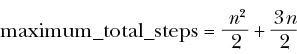
We finally have a very precise expression for the maximum total steps that could be required to perform insertion sort. But believe it or not, this expression may even be too precise, for several reasons. One is that it’s the maximum number of steps required, but the minimum and the average could be much lower, and almost every conceivable list that we might want to sort would require fewer steps. Remember the jaggedness in the curve we plotted in Figure 4-1—there’s always variation in how long it takes to perform an algorithm, depending on our choice of input.
Another reason that our expression for the maximum steps could be called too precise is that knowing the number of steps for an algorithm is most important for large values of n, but as n gets very large, a small part of the expression starts to dominate the rest in importance because of the sharply diverging growth rates of different functions.
Consider the expression n2 + n. It is a sum of two terms: an n2 term, and an n term. When n = 10, n2 + n is 110, which is 10% higher than n2. When n = 100, n2 + n is 10,100, which is only 1% higher than n2. As n grows, the n2 term in the expression becomes more important than the n term because quadratic functions grow so much faster than linear ones. So if we have one algorithm that takes n2+ n steps to perform and another algorithm that takes n2 steps to perform, as n grows very large, the difference between them will matter less and less. Both of them run in more or less n2 steps.
Using Big O Notation
To say that an algorithm runs in more or less n2 steps is a reasonable balance between the precision we want and the conciseness we want (and the randomness we have). The way we express this type of “more or less” relationship formally is by using big O notation(the O is short for order). We might say that a particular algorithm is “big O of n2,” or O(n2), if, in the worst case, it runs in more or less n2 steps for large n. The technical definition states that the function f(x) is big- O of the function g(x) if there’s some constant number M such that the absolute value of f(x) is always less than M times g(x) for all sufficiently large values of x.
In the case of insertion sort, when we look at our expression for the maximum number of steps required to perform the algorithm, we find that it’s a sum of two terms: one is a multiple of n2, and the other is a multiple of n. As we just discussed, the term that is a multiple of n will matter less and less as n grows, and the n2 term will come to be the only one that we are concerned with. So the worst case of insertion sort is that it is a O(n2) (“big O of n2”) algorithm.
The quest for algorithm efficiency consists of seeking algorithms whose runtimes are big O of smaller and smaller functions. If we could find a way to alter insertion sort so that it is O(n1.5) instead of O(n2), that would be a major breakthrough that would make a huge difference in runtimes for large values of n. We can use big O notation to talk not only about time but also about space. Some algorithms can gain speed by storing big datasets in memory. They might be big O of a small function for runtime but big O of a larger function for memory requirements. Depending on the circumstances, it may be wise to gain speed by eating up memory, or to free up memory by sacrificing speed. In this chapter, we’ll focus on gaining speed and designing algorithms to have runtimes that are big O of the smallest possible functions, without regard to memory requirements.
After learning insertion sort and seeing that its runtime performance is O(n2), it’s natural to wonder what level of improvement we can reasonably hope for. Could we find some holy grail algorithm that could sort any possible list in fewer than 10 steps? No. Every sorting algorithm will require at least n steps, because it will be necessary to consider each element of the list in turn, for each of the n elements. So any sorting algorithm will be at least O(n). We cannot do better than O(n), but can we do better than insertion sort’s O(n2)? We can. Next, we’ll consider an algorithm that’s known to be O(nlog(n)), a significant improvement over insertion sort.
Merge Sort
Merge sort is an algorithm that’s much quicker than insertion sort. Just like insertion sort, merge sort contains two parts: a part that merges two lists and a part that repeatedly uses merging to accomplish the actual sorting. Let’s consider the merging itself before we consider the sorting.
Suppose we have two filing cabinets that are both sorted individually but have never been compared to each other. We want to combine their contents into one final filing cabinet that is also completely sorted. We will call this task a merge of the two sorted filing cabinets. How should we approach this problem?
Once again, it’s worthwhile to consider how we would do this with real filing cabinets before we open Python and start writing code. In this case, we can imagine having three filing cabinets in front of us: the two full, sorted filing cabinets whose files we want to merge, and a third, empty filing cabinet that we will insert files into and that will eventually contain all of the files from the original two cabinets. We can call our two original cabinets the “left” and “right” cabinets, imagining that they are placed on our left and right.
Merging
To merge, we can take the first file in both of the original cabinets simultaneously: the first left file with our left hand and the first right file with our right hand. Whichever file is lower is inserted into the new cabinet as its first file. To find the second file for the new cabinet, once again take the first file in the left and right cabinets, compare them, and insert whichever is lower into the last position in the new cabinet. When either the left cabinet or the right cabinet is empty, take the remaining files in the non-empty cabinet and place them all together at the end of the new cabinet. After this, your new cabinet will contain all the files from the left and right cabinets, sorted in order. We have successfully merged our original two cabinets.
In Python, we’ll use the variables left and right to refer to our original sorted cabinets, and we’ll define a newcabinet list, which will start empty and eventually contain all elements of both left and right, in order.
newcabinet = []We’ll define example cabinets that we’ll call left and right:
left = [1,3,4,4,5,7,8,9]
right = [2,4,6,7,8,8,10,12,13,14]
To compare the respective first elements of our left and right cabinets, we’ll use the following if statements (which won’t be ready to run until we fill in the --snip-- sections):
   if left[0] > right[0]:
    --snip--
   elif left[0] <= right[0]:
    --snip--
Remember that if the first element of the left cabinet is lower than the first element of the right cabinet, we want to pop that element out of the left cabinet and insert it into the newcabinet, and vice versa. We can accomplish that by using Python’s built-in pop() function, inserting it into our if statements as follows:
if left[0] > right[0]:
    to_insert = right.pop(0)
    newcabinet.append(to_insert)
elif left[0] <= right[0]:
    to_insert = left.pop(0)
    newcabinet.append(to_insert)
This process—checking the first elements of the left and right cabinets and popping the appropriate one into the new cabinet—needs to continue as long as both of the cabinets still have at least one file. That’s why we will nest these if statements inside a while loop that checks the minimum length of left and right. As long as both left and right contain at least one file, it will continue its process:
while(min(len(left),len(right)) > 0):
    if left[0] > right[0]:
        to_insert = right.pop(0)
        newcabinet.append(to_insert)
    elif left[0] <= right[0]:
        to_insert = left.pop(0)
        newcabinet.append(to_insert)
Our while loop will stop executing as soon as either left or right runs out of files to insert. At that point, if left is empty, we’ll insert all the files in right at the end of the new cabinet in their current order, and vice versa. We can accomplish that final insertion as follows:
if(len(left) > 0):
    for i in left:
        newcabinet.append(i)

if(len(right) > 0):
    for i in right:
        newcabinet.append(i)
Finally, we combine all of those snippets into our final merging algorithm in Python as shown in Listing 4-4.
def merging(left,right):
    newcabinet = []
    while(min(len(left),len(right)) > 0):
        if left[0] > right[0]:
            to_insert = right.pop(0)
            newcabinet.append(to_insert)
        elif left[0] <= right[0]:
            to_insert = left.pop(0)
            newcabinet.append(to_insert)
    if(len(left) > 0):
        for i in left:
            newcabinet.append(i)
    if(len(right)>0):
        for i in right:
            newcabinet.append(i)
    return(newcabinet)

left = [1,3,4,4,5,7,8,9]
right = [2,4,6,7,8,8,10,12,13,14]

newcab=merging(left,right)
Listing 4-4: An algorithm to merge two sorted lists
The code in Listing 4-4 creates newcab, a single list that contains all elements of left and right, merged and in order. You can run print(newcab) to see that our merging function worked.
From Merging to Sorting
Once we know how to merge, merge sort is within our grasp. Let’s start by creating a simple merge sort function that works only on lists that have two or fewer elements. A one-element list is already sorted, so if we pass that as the input to our merge sort function, we should just return it unaltered. If we pass a two-element list to our merge sort function, we can split that list into two one-element lists (that are therefore already sorted) and call our merging function on those one-element lists to get a final, sorted two-element list. The following Python function accomplishes what we need:
import math

def mergesort_two_elements(cabinet):
    newcabinet = []
    if(len(cabinet) == 1):
        newcabinet = cabinet
    else:
        left = cabinet[:math.floor(len(cabinet)/2)]
        right = cabinet[math.floor(len(cabinet)/2):]
        newcabinet = merging(left,right)
    return(newcabinet)
This code relies on Python’s list indexing syntax to split whatever cabinet we want to sort into a left cabinet and a right cabinet. You can see in the lines that define left and right that we’re using :math.floor(len(cabinet)/2) and math.floor(len(cabinet)/2): to refer to the entire first half or the entire second half of the original cabinet, respectively. You can call this function with any one- or two-element cabinet—for example, mergesort_two_elements([3,1])—and see that it successfully returns a sorted cabinet.
Next, let’s write a function that can sort a list that has four elements. If we split a four-element list into two sublists, each sublist will have two elements. We could follow our merging algorithm to combine these lists. However, recall that our merging algorithm is designed to combine two already sorted lists. These two lists may not be sorted, so using our merging algorithm will not successfully sort them. However, each of our sublists has only two elements, and we just wrote a function that can perform merge sort on lists with two elements. So we can split our four-element list into two sublists, call our merge sort function that works on two-element lists on each of those sublists, and then merge the two sorted lists together to get a sorted result with four elements. This Python function accomplishes that:
def mergesort_four_elements(cabinet):
    newcabinet = []
    if(len(cabinet) == 1):
        newcabinet = cabinet
    else:
        left = mergesort_two_elements(cabinet[:math.floor(len(cabinet)/2)])
        right = mergesort_two_elements(cabinet[math.floor(len(cabinet)/2):])
        newcabinet = merging(left,right)
    return(newcabinet)

cabinet = [2,6,4,1]
newcabinet = mergesort_four_elements(cabinet)
We could continue writing these functions to work on successively larger lists. But the breakthrough comes when we realize that we can collapse that whole process by using recursion. Consider the function in Listing 4-5, and compare it to the preceding mergesort_four_elements() function.
def mergesort(cabinet):
    newcabinet = []
    if(len(cabinet) == 1):
        newcabinet = cabinet
    else:
   1 left = mergesort(cabinet[:math.floor(len(cabinet)/2)])
   2 right = mergesort(cabinet[math.floor(len(cabinet)/2):])
        newcabinet = merging(left,right)
    return(newcabinet)
Listing 4-5: Implementing merge sort with recursion
You can see that this function is nearly identical to our mergesort_four_elements() to function. The crucial difference is that to create the sorted left and right cabinets, it doesn’t call another function that works on smaller lists. Rather, it calls itself on the smaller list 12. Merge sort is a divide and conquer algorithm. We start with a large, unsorted list. Then we split that list repeatedly into smaller and smaller chunks (the dividing) until we end up with sorted (conquered) one-item lists, and then we simply merge them back together successively until we have built back up to one big sorted list. We can call this merge sort function on a list of any size and check that it works:
cabinet = [4,1,3,2,6,3,18,2,9,7,3,1,2.5,-9]
newcabinet = mergesort(cabinet)
print(newcabinet)
When we put all of our merge sort code together, we get Listing 4-6.
def merging(left,right):
    newcabinet = []
    while(min(len(left),len(right)) > 0):
        if left[0] > right[0]:
            to_insert = right.pop(0)
            newcabinet.append(to_insert)
        elif left[0] <= right[0]:
            to_insert = left.pop(0)
            newcabinet.append(to_insert)
    if(len(left) > 0):
        for i in left:
            newcabinet.append(i)
    if(len(right) > 0):
        for i in right:
            newcabinet.append(i)
    return(newcabinet)

import math

def mergesort(cabinet):
    newcabinet = []
    if(len(cabinet) == 1):
        newcabinet=cabinet
    else:
        left = mergesort(cabinet[:math.floor(len(cabinet)/2)])
        right = mergesort(cabinet[math.floor(len(cabinet)/2):])
        newcabinet = merging(left,right)
    return(newcabinet)

cabinet = [4,1,3,2,6,3,18,2,9,7,3,1,2.5,-9]
newcabinet=mergesort(cabinet)
Listing 4-6: Our complete merge sort code
You could add a step counter to your merge sort code to check how many steps it takes to run and how it compares to insertion sort. The merge sort process consists of successively splitting the initial cabinet into sublists and then merging those sublists back together, preserving the sorting order. Every time we split a list, we’re cutting it in half. The number of times a list of length n can be split in half before each sublist has only one element is about log(n) (where the log is to base 2), and the number of comparisons we have to make at each merge is at most n. So n or fewer comparisons for each of log(n) comparisons means that merge sort is O(n×log(n)), which may not seem impressive but actually makes it the state of the art for sorting. In fact, when we call Python’s built-in sorting function sorted as follows:
print(sorted(cabinet))Python is using a hybrid version of merge sort and insertion sort behind the scenes to accomplish this sorting task. By learning merge sort and insertion sort, you’ve gotten up to speed with the quickest sorting algorithm computer scientists have been able to create, something that is used millions of times every day in every imaginable kind of application.
Sleep Sort
The enormous negative influence that the internet has had on humanity is occasionally counterbalanced by a small, shining treasure that it provides. Occasionally, the bowels of the internet even produce a scientific discovery that creeps into the world outside the purview of scientific journals or the “establishment.” In 2011, an anonymous poster on the online image board 4chan proposed and provided code for a sorting algorithm that had never been published before and has since come to be called sleep sort.
Sleep sort wasn’t designed to resemble any real-world situation, like inserting files into a filing cabinet. If we’re seeking an analogy, we might consider the task of allocating lifeboat spots on the Titanic as it began to sink. We might want to allow children and younger people the first chance to get on the lifeboats, and then allow older people to try to get one of the remaining spots. If we make an announcement like “younger people get on the boats before older people,” we’d face chaos as everyone would have to compare their ages—they would face a difficult sorting problem amidst the chaos of the sinking ship.
A sleep-sort approach to the Titanic lifeboats would be the following. We would announce, “Everyone please stand still and count to your age: 1, 2, 3, . . . . As soon as you have counted up to your current age, step forward to get on a lifeboat.” We can imagine that 8-year-olds would finish their counting about one second before the 9-year-olds, and so would have a one-second head start and be able to get a spot on the boats before those who were 9. The 8- and 9-year-olds would similarly be able to get on the boats before the 10-year-olds, and so on. Without doing any comparisons at all, we’d rely on individuals’ ability to pause for a length of time proportional to the metric we want to sort on and then insert themselves, and the sorting would happen effortlessly after that—with no direct inter-person comparisons.
This Titanic lifeboat process shows the idea of sleep sort: allow each element to insert itself directly, but only after a pause in proportion to the metric it’s being sorted on. From a programming perspective, these pauses are called sleeps and can be implemented in most languages.
In Python, we can implement sleep sort as follows. We will import the threading module, which will enable us to create different computer processes for each element of our list to sleep and then insert itself. We’ll also import the time.sleep module, which will enable us to put our different “threads” to sleep for the appropriate length of time.
import threading
from time import sleep

def sleep_sort(i):
    sleep(i)
    global sortedlist
    sortedlist.append(i)
    return(i)

items = [2, 4, 5, 2, 1, 7]
sortedlist = []
ignore_result = [threading.Thread(target = sleep_sort, args = (i,)).start() for i in items]
The sorted list will be stored in the sortedlist variable, and you can ignore the list we create called ignore_result. You can see that one advantage of sleep sort is that it can be written concisely in Python. It’s also fun to print the sortedlist variable before the sorting is done (in this case, within about 7 seconds) because depending on exactly when you execute the print command, you’ll see a different list. However, sleep sort also has some major disadvantages. One of these is that because it’s not possible to sleep for a negative length of time, sleep sort cannot sort lists with negative numbers. Another disadvantage is that sleep sort’s execution is highly dependent on outliers—if you append 1,000 to the list, you’ll have to wait at least 1,000 seconds for the algorithm to finish executing. Yet another disadvantage is that numbers that are close to each other may be inserted in the wrong order if the threads are not executed perfectly concurrently. Finally, since sleep sort uses threading, it will not be able to execute (well) on hardware or software that does not enable threading (well).
If we had to express sleep sort’s runtime in big O notation, we might say that it is O(max(list)). Unlike the runtime of every other well-known sorting algorithm, its runtime depends not on the size of the list but on the size of the elements of the list. This makes sleep sort hard to rely on, because we can only be confident about its performance with certain lists—even a short list may take far too long to sort if any of its elements are too large.
There may never be a practical use for sleep sort, even on a sinking ship. I include it here for a few reasons. First, because it is so different from all other extant sorting algorithms, it reminds us that even the most stale and static fields of research have room for creativity and innovation, and it provides a refreshingly new perspective on what may seem like a narrow field. Second, because it was designed and published anonymously and probably by someone outside the mainstream of research and practice, it reminds us that great thoughts and geniuses are found not only in fancy universities, established journals, and top firms, but also among the uncredentialed and unrecognized. Third, it represents a fascinating new generation of algorithms that are “native to computers,” meaning that they are not a translation of something that can be done with a cabinet and two hands like many old algorithms, but are fundamentally based on capabilities that are unique to computers (in this case, sleeping and threading). Fourth, the computer-native ideas it relies on (sleeping and threading) are very useful and worth putting in any algorithmicist’s toolbox for use in designing other algorithms. And fifth, I have an idiosyncratic affection for it, maybe just because it is a strange, creative misfit or maybe because I like its method of self-organizing order and the fact that I can use it if I’m ever in charge of saving a sinking ship.
From Sorting to Searching
Searching, like sorting, is fundamental to a variety of tasks in computer science (and in the rest of life). We may want to search for a name in a phone book, or (since we’re living after the year 2000) we may need to access a database and find a relevant record.
Searching is often merely a corollary of sorting. In other words, once we have sorted a list, searching is very straightforward—the sorting is often the hard part.
Binary Search
Binary search is a quick and effective method for searching for an element in a sorted list. It works a little like a guessing game. Suppose that someone is thinking of a number from 1 to 100 and you are trying to guess it. You may guess 50 as your first guess. Your friend says that 50 is incorrect but allows you to guess again and gives you a hint: 50 is too high. Since 50 is too high, you guess 49. Again, you are incorrect, and your friend tells you that 49 is too high and gives you another chance to guess. You could guess 48, then 47, and so on until you get the right answer. But that could take a long time—if the correct number is 1, it will take you 50 guesses to get it, which seems like too many guesses considering there were only 100 total possibilities to begin with.
A better approach is to take larger jumps after you find out whether your guess is too high or too low. If 50 is too high, consider what we could learn from guessing 40 next instead of 49. If 40 is too low, we have eliminated 39 possibilities (1–39) and we’ll definitely be able to guess in at most 9 more guesses (41–49). If 40 is too high, we’ve at least eliminated 9 possibilities (41–49) and we’ll definitely be able to guess in at most 39 more guesses (1–39). So in the worst case, guessing 40 narrows down the possibilities from 49 (1–49) to 39 (1–39). By contrast, guessing 49 narrows down the possibilities from 49 (1–49) to 48 (1–48) in the worst case. Clearly, guessing 40 is a better searching strategy than guessing 49.
It turns out that the best searching strategy is to guess exactly the midpoint of the remaining possibilities. If you do that and then check whether your guess was too high or too low, you can always eliminate half of the remaining possibilities. If you eliminate half of the possibilities in each round of guessing, you can actually find the right value quite quickly (O(log(n)) for those keeping score at home). For example, a list with 1,000 items will require only 10 guesses to find any element with a binary search strategy. If we’re allowed to have only 20 guesses, we can correctly find the position of an element in a list with more than a million items. Incidentally, this is why we can write guessing-game apps that can correctly “read your mind” by asking only about 20 questions.
To implement this in Python, we will start by defining upper and lower bounds for what location a file can occupy in a filing cabinet. The lower bound will be 0, and the upper bound will be the length of the cabinet:
sorted_cabinet = [1,2,3,4,5]
upperbound = len(sorted_cabinet)
lowerbound = 0
To start, we will guess that the file is in the middle of the cabinet. We’ll import Python’s math library to use the floor() function, which can convert decimals to integers. Remember that guessing the halfway point gives us the maximum possible amount of information:
import math
guess = math.floor(len(sorted_cabinet)/2)
Next, we will check whether our guess is too low or too high. We’ll take a different action depending on what we find. We use the looking_for variable for the value we are searching for:
if(sorted_cabinet[guess] > looking_for):
    --snip--
if(sorted_cabinet[guess] < looking_for):
    --snip--
If the file in the cabinet is too high, then we’ll make our guess the new upper bound, since there is no use looking any higher in the cabinet. Then our new guess will be lower—to be precise, it will be halfway between the current guess and the lower bound:
looking_for = 3
if(sorted_cabinet[guess] > looking_for):
    upperbound = guess
    guess = math.floor((guess + lowerbound)/2)
We follow an analogous process if the file in the cabinet is too low:
if(sorted_cabinet[guess] < looking_for):
    lowerbound = guess
    guess = math.floor((guess + upperbound)/2)
Finally, we can put all of these pieces together into a binarysearch() function. The function contains a while loop that will run for as long as it takes until we find the part of the cabinet we’ve been looking for (Listing 4-7).
import math
sortedcabinet = [1,2,3,4,5,6,7,8,9,10]

def binarysearch(sorted_cabinet,looking_for):
    guess = math.floor(len(sorted_cabinet)/2)
    upperbound = len(sorted_cabinet)
    lowerbound = 0
    while(abs(sorted_cabinet[guess] - looking_for) > 0.0001):
        if(sorted_cabinet[guess] > looking_for):
            upperbound = guess
            guess = math.floor((guess + lowerbound)/2)
        if(sorted_cabinet[guess] < looking_for):
            lowerbound = guess
            guess = math.floor((guess + upperbound)/2)
    return(guess)

print(binarysearch(sortedcabinet,8))
Listing 4-7: An implementation of binary search
The final output of this code tells us that the number 8 is at position 7 in our sorted_cabinet. This is correct (remember that the index of Python lists starts at 0). This strategy of guessing in a way that eliminates half of the remaining possibilities is useful in many domains. For example, it’s the basis for the most efficient strategy on average in the formerly popular board game Guess Who. It’s also the best way (in theory) to look words up in a large, unfamiliar dictionary.
Applications of Binary Search
Besides guessing games and word lookups, binary search is used in a few other domains. For example, we can use the idea of binary search when debugging code. Suppose that we have written some code that doesn’t work, but we aren’t sure which part is faulty. We can use a binary search strategy to find the problem. We split the code in half and run both halves separately. Whichever half doesn’t run properly is the half where the problem lies. Again, we split the problematic part in half, and test each half to further narrow down the possibilities until we find the offending line of code. A similar idea is implemented in the popular code version-control software Git as git bisect (although gitbisect iterates through temporally separated versions of the code rather than through lines in one version).
Another application of binary search is inverting a mathematical function. For example, imagine that we have to write a function that can calculate the arcsin, or inverse sine, of a given number. In only a few lines, we can write a function that will call our binarysearch() function to get the right answer. To start, we need to define a domain; these are the values that we will search through to find a particular arcsin value. The sine function is periodic and takes on all of its possible values between –pi/2 and pi/2, so numbers in between those extremes will constitute our domain. Next, we calculate sine values for each value in the domain. We call binarysearch() to find the position of the number whose sine is the number we’re looking for, and return the domain value with the corresponding index, like so:
def inverse_sin(number):
    domain = [x * math.pi/10000 - math.pi/2 for x in list(range(0,10000))]
    the_range = [math.sin(x) for x in domain]
    result = domain[binarysearch(the_range,number)]
    return(result)
You can run inverse_sin(0.9) and see that this function returns the correct answer: about 1.12.
This is not the only way to invert a function. Some functions can be inverted through algebraic manipulation. However, algebraic function inversion can be difficult or even impossible for many functions. The binary search method presented here, by contrast, can work for any function, and with its O(log(n)) runtime, it’s also lightning fast.
Summary
Sorting and searching may feel mundane to you, as if you’ve taken a break from an adventure around the world to attend a seminar on folding laundry. Maybe so, but remember that if you can fold clothes efficiently, you can pack more gear for your trek up Kilimanjaro. Sorting and searching algorithms can be enablers, helping you build newer and greater things on their shoulders. Besides that, it’s worth studying sorting and searching algorithms closely because they are fundamental and common, and the ideas you see in them can be useful for the rest of your intellectual life. In this chapter, we discussed some fundamental and interesting sorting algorithms, plus binary search. We also discussed how to compare algorithms and use big O notation.
In the next chapter, we’ll turn to a few applications of pure math. We’ll see how we can use algorithms to explore the mathematical world, and how the mathematical world can help us understand our own.