The quantitative precision of algorithms makes them naturally suited to applications in mathematics. In this chapter, we explore algorithms that are useful in pure mathematics and look at how mathematical ideas can improve any of our algorithms. We’ll start by discussing continued fractions, an austere topic that will take us to the dizzy­ing heights of the infinite and give us the power to find order in chaos. We’ll continue by discussing square roots, a more prosaic but arguably more useful topic. Finally, we’ll discuss randomness, including the mathematics of randomness and some important algorithms that generate random numbers.

Continued Fractions

In 1597, the great Johannes Kepler wrote about what he considered geometry’s “two great treasures”: the Pythagorean theorem and a number that has since come to be called the golden ratio. Often denoted by the Greek letter phi, the golden ratio is equal to about 1.618, and Kepler was only one of dozens of great thinkers who have been entranced by it. Like pi and a few other famous constants, such as the exponential base e, phi has a tendency to show up in unexpected places. People have found phi in many places in nature, and have painstakingly documented where it occurs in fine art, as in the annotated version of the Rokeby Venus shown in Figure 5-1.

In Figure 5-1, a phi enthusiast has added overlays that indicate that the ratios of some of these lengths, like b/a and d/c, seem to be equal to phi. Many great paintings have a composition that’s amenable to this kind of phi-hunting.

Compressing and Communicating Phi

Phi’s exact value is surprisingly hard to express. I could say that it’s equal to 1.61803399 . . . . The ellipsis here is a way of cheating; it means that more numbers follow (an infinite number of numbers, in fact), but I haven’t told you what those numbers are, so you still don’t know the exact value of phi.

For some numbers with infinite decimal expansions, a fraction can represent them exactly. For example, the number 0.11111 . . . is equal to 1/9—here, the fraction provides an easy way to express the exact value of an infinitely continued decimal. Even if you didn’t know the fractional representation, you could see the pattern of repeating 1s in 0.1111 . . . and thereby understand its exact value. Unfortunately, the golden ratio is what’s called an irrational number, meaning that there are no two integers x and y that enable us to say that phi is equal to x/y. Moreover, no one has yet been able to discern any pattern in its digits.

We have an infinite decimal expansion with no clear pattern and no fractional representation. It may seem impossible to ever clearly express phi’s exact value. But if we learn more about phi, we can find a way to express it both exactly and concisely. One of the things we know about phi is that it’s the solution to this equation:

One way we might imagine expressing the exact value of phi would be to write “the solution to the equation written above this paragraph.” This has the benefit of being concise and technically exact, but it means that we have to solve the equation somehow. That description also doesn’t tell us the 200th or 500th digit in phi’s expansion.

If we divide our equation by phi, we get the following:

And if we rearrange that equation, we get this:

Now imagine if we attempted a strange substitution of this equation into itself:

Here, we rewrote the phi on the righthand side as 1 + 1/phi. We could do that same substitution again; why not?

We can perform this substitution as many times as we like, with no end. As we continue, phi gets pushed more and more levels “in” to the corner of a growing fraction. Listing 5-1 shows an expression for phi with phi seven levels in.

Listing 5-1: A continued fraction with seven levels expressing the value of phi

If we imagine continuing this process, we can push phi infinity levels in. Then what we have left is shown in Listing 5-2.

Listing 5-2: An infinite continued fraction expressing the value of phi

In theory, after the infinity of 1s and plus signs and fraction bars represented by the ellipsis, we should insert a phi into Listing 5-2, just like it appears in the bottom right of Listing 5-1. But we will never get through all of those 1s (because there are an infinite number of them), so we are justified in forgetting entirely about the phi that’s supposed to be nested in the righthand side.

More about Continued Fractions

The expressions just shown are called continued fractions. A continued fraction consists of sums and reciprocals nested in multiple layers. Continued fractions can be finite, like the one in Listing 5-1 that terminated after seven layers, or infinite, continuing forever without end like the one in Listing 5-2. Continued fractions are especially useful for our purposes because they enable us to express the exact value of phi without needing to chop down an infinite forest to manufacture enough paper. In fact, mathematicians sometimes use an even more concise notation method that enables us to express a continued fraction in one simple line. Instead of writing all the fraction bars in a continued fraction, we can use square brackets ([ ]) to denote that we’re working with a continued fraction, and use a semicolon to separate the digit that’s “alone” from the digits that are together in a fraction. With this method, we can write the continued fraction for phi as the following:

In this case, the ellipses are no longer losing information, since the continued fraction for phi has a clear pattern: it’s all 1s, so we know its exact 100th or 1,000th element. This is one of those times when mathematics seems to deliver something miraculous to us: a way to concisely write down a number that we had thought was infinite, without pattern, and ineffable. But phi isn’t the only possible continued fraction. We could write another continued fraction as follows:

In this case, after the first few digits, we find a simple pattern: pairs of 1s alternate with increasing even numbers. The next values will be 1, 1, 10, 1, 1, 12, and so on. We can write the beginning of this continued fraction in a more conventional style as

In fact, this mystery number is none other than our old friend e, the base of the natural logarithm! The constant e, just like phi and other irrational numbers, has an infinite decimal expansion with no apparent pattern and cannot be represented by a finite fraction, and it seems like it’s impossible to express its exact numeric value concisely. But by using the new concept of continued fractions and a new concise notation, we can write these apparently intractable numbers in one line. There are also several remarkable ways to use continued fractions to represent pi. This is a victory for data compression. It’s also a victory in the perennial battle between order and chaos: where we thought there was nothing but encroaching chaos dominating the numbers we love, we find that there was always a deep order beneath the surface.

Our continued fraction for phi came from a special equation that works only for phi. But in fact, it is possible to generate a continued fraction representation of any number.

An Algorithm for Generating Continued Fractions

To find a continued fraction expansion for any number, we’ll use an algorithm.

It’s easiest to find continued fraction expansions for numbers that are integer fractions already. For example, consider the task of finding a continued fraction representation of 105/33. Our goal is to express this number in a form that looks like the following:

where the ellipses could be referring to a finite rather than an infinite continuation. Our algorithm will generate a first, then b, then c, and proceed through terms of the alphabet sequentially until it reaches the final term or until we require it to stop.

If we interpret our example 105/33 as a division problem instead of a fraction, we find that 105/33 is 3, remainder 6. We can rewrite 105/33 as 3 + 6/33:

The left and the right sides of this equation both consist of an integer (3 and a) and a fraction (6/33 and the rest of the right side). We conclude that the integer parts are equal, so a = 3. After this, we have to find a suitable b, c, and so on such that the whole fractional part of the expression will evaluate to 6/33.

To find the right b, c, and the rest, look at what we have to solve after concluding that a = 3:

If we take the reciprocal of both sides of this equation, we get the following equation:

Our task is now to find b and c. We can do a division again; 33 divided by 6 is 5, with remainder 3, so we can rewrite 33/6 as 5 + 3/6:

We can see that both sides of the equation have an integer (5 and b) and a fraction (3/6 and the rest of the right side). We can conclude that the integer parts are equal, so b = 5. We have gotten another letter of the alphabet, and now we need to simplify 3/6 to progress further. If you can’t tell immediately that 3/6 is equal to 1/2, you could follow the same process we did for 6/33: say that 3/6 expressed as a reciprocal is 1/(6/3), and we find that 6/3 is 2 remainder 0. The algorithm we’re following is meant to complete when we have a remainder of 0, so we will realize that we’ve finished the process, and we can write our full continued fraction as in Listing 5-3.

Listing 5-3: A continued fraction for 105/33

If this process of repeatedly dividing two integers to get a quotient and a remainder felt familiar to you, it should have. In fact, it’s the same process we followed in Euclid’s algorithm in Chapter 2! We follow the same steps but record different answers: for Euclid’s algorithm, we recorded the final nonzero remainder as the final answer, and in the continued fraction generation algorithm, we recorded every quotient (every letter of the alphabet) along the way. As happens so often in math, we have found an unexpected connection—in this case, between the generation of a continued fraction and the discovery of a greatest common divisor.

We can implement this continued fraction generation algorithm in Python as follows.

We’ll assume that we’re starting with a fraction of the form x/y. First, we decide which of x and y is bigger and which is smaller:

x = 105
y = 33
big = max(x,y)
small = min(x,y)

Next, we’ll take the quotient of the bigger divided by the smaller of the two, just as we did with 105/33. When we found that the result was 3, remainder 6, we concluded that 3 was the first term (a) in the continued fraction. We can take this quotient and store the result as follows:

import math
output = []
quotient = math.floor(big/small)
output.append(quotient)

In this case, we are ready to obtain a full alphabet of results (a, b, c, and so on), so we create an empty list called output and append our first result to it.

Finally, we have to repeat the process, just as we did for 33/6. Remember that 33 was previously the small variable, but now it’s the big one, and the remainder of our division process is the new small variable. Since the remainder is always smaller than the divisor, big and small will always be correctly labeled. We accomplish this switcheroo in Python as follows:

new_small = big % small
big = small
small = new_small

At this point, we have completed one round of the algorithm, and we need to repeat it for our next set of numbers (33 and 6). In order to accomplish the process concisely, we can put it all in a loop, as in Listing 5-4.

import math
def continued_fraction(x,y,length_tolerance):
    output = []
    big = max(x,y)
    small = min(x,y)
    
    while small > 0 and len(output) < length_tolerance:
        quotient = math.floor(big/small)
        output.append(quotient)
        new_small = big % small
        big = small
        small = new_small
    return(output)

Listing 5-4: An algorithm for expressing fractions as continued fractions

Here, we took x and y as inputs, and we defined a length_tolerance variable. Remember that some continued fractions are infinite in length, and others are extremely long. By including a length_tolerance variable in the function, we can stop our process early if the output is getting unwieldy, and thereby avoid getting caught in an infinite loop.

Remember that when we performed Euclid’s algorithm, we used a recursive solution. In this case, we used a while loop instead. Recursion is well suited to Euclid’s algorithm because it required only one final output number at the very end. Here, however, we want to collect a sequence of numbers in a list. A loop is better suited to that kind of sequential collection.

We can run our new continued_fraction generation function as follows:

print(continued_fraction(105,33,10))

We’ll get the following simple output:

[3,5,2]

We can see that the numbers here are the same as the key integers on the right side of Listing 5-3.

We may want to check that a particular continued fraction correctly expresses a number we’re interested in. In order to do this, we should define a get_number() function that converts a continued fraction to a decimal number, as in Listing 5-5.

def get_number(continued_fraction):
    index = -1
    number = continued_fraction[index]
    
    while abs(index) < len(continued_fraction):
        next = continued_fraction[index - 1]
        number = 1/number + next
        index -= 1
    return(number)  

Listing 5-5: Converting a continued fraction to a decimal representation of a number

We don’t need to worry about the details of this function since we’re just using it to check our continued fractions. We can check that the function works by running get_number([3,5,2]) and seeing that we get 3.181818 . . . as the output, which is another way to write 105/33 (the number we started with).

From Decimals to Continued Fractions

What if, instead of starting with some x/y as an input to our continued fraction algorithm, we start with a decimal number, like 1.4142135623730951? We’ll need to make a few adjustments, but we can more or less follow the same process we followed for fractions. Remember that our goal is to find a, b, c, and the rest of the alphabet in the following type of expression:

Finding a is as simple as it gets—it’s just the part of the decimal number to the left of the decimal point. We can define this first_term (a in our equation) and the leftover as follows:

x = 1.4142135623730951
output = []
first_term = int(x)
leftover = x - int(x)
output.append(first_term)

Just like before, we’re storing our successive answers in a list called output.

After solving for a, we have a leftover, and we need to find a continued fraction representation for it:

Again, we can take a reciprocal of this:

Our next term, b, will be the integer part to the left of the decimal point in this new term—in this case, 2. And then we will repeat the process: taking a reciprocal of a decimal part, finding the integer part to the left of the decimal, and so on.

In Python, we accomplish each round of this as follows:

next_term = math.floor(1/leftover)
leftover = 1/leftover - next_term
output.append(next_term)

We can put the whole process together into one function as in Listing 5-6.

def continued_fraction_decimal(x,error_tolerance,length_tolerance):
    output = []
    first_term = int(x)
    leftover = x - int(x)
    output.append(first_term)
    error = leftover
    while error > error_tolerance and len(output) <length_tolerance:
        next_term = math.floor(1/leftover)
        leftover = 1/leftover - next_term
        output.append(next_term)
        error = abs(get_number(output) - x)
    return(output)

Listing 5-6: Finding continued fractions from decimal numbers

In this case, we include a length_tolerance term just like before. We also add an error_tolerance term, which allows us to exit the algorithm if we get an approximation that’s “close enough” to the exact answer. To find out whether we are close enough, we take the difference between x, the number we are trying to approximate, and the decimal value of the continued fraction terms we have calculated so far. To get that decimal value, we can use the same get_number() function we wrote in Listing 5-5.

We can try our new function easily as follows:

print(continued_fraction_decimal(1.4142135623730951,0.00001,100))

We get the following output:

[1, 2, 2, 2, 2, 2, 2, 2]

We can write this continued fraction as follows (using an approximate equal sign because our continued fraction is an approximation to within a tiny error and we don’t have the time to calculate every element of an infinite sequence of terms):

Notice that there are 2s all along the diagonal in the fraction on the right. We’ve found the first seven terms of another infinite continued fraction whose infinite expansion consists of all 2s. We could write its continued fraction expansion as [1,2,2,2,2, . . .]. This is the continued fraction expansion of √2, another irrational number that can’t be represented as an integer fraction, has no pattern in its decimal digit, and yet has a convenient and easily memorable representation as a continued fraction.

From Fractions to Radicals

If you’re interested in continued fractions, I recommend that you read about Srinivasa Ramanujan, who during his short life traveled mentally to the edges of infinity and brought some gems back for us to treasure. In addition to continued fractions, Ramanujan was interested in continued square roots (also known as nested radicals)—for example, the following three infinitely nested radicals:

and

and

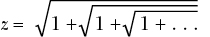
It turns out that x = 2 (an old anonymous result), y = 3 (as proved by Ramanujan), and z is none other than phi, the golden ratio! I encourage you to try to think of a method for generating nested radical representations in Python. Square roots are obviously interesting if we take them to infinite lengths, but it turns out that they’re interesting even if we just consider them alone.

Square Roots

We take handheld calculators for granted, but when we think about what they can do, they’re actually quite impressive. For example, you may remember learning in geometry class that the sine is defined in terms of triangle lengths: the length of the angle’s opposite side divided by the length of the hypotenuse. But if that is the definition of a sine, how can a calculator have a sin button that performs this calculation instantaneously? Does the calculator draw a right triangle in its innards, get out a ruler and measure the lengths of the sides, and then divide them? We might ask a similar question for square roots: the square root is the inverse of a square, and there’s no straightforward, closed-form arithmetic formula for it that a calculator could use. I imagine that you can already guess the answer: there is an algorithm for quick calculations of square roots.

The Babylonian Algorithm

Suppose that we need to find the square root of a number x. As with any math problem, we can try a guess-and-check strategy. Let’s say that our best guess for the square root of x is some number y. We can calculate y², and if it’s equal to x, we’re done (having achieved a rare completion of the one-step “lucky guess algorithm”).

If our guess y is not exactly the square root of x, then we’ll want to guess again, and we’ll want our next guess to take us closer to the true value of the square root of x. The Babylonian algorithm provides a way to systematically improve our guesses until we converge on the right answer. It’s a simple algorithm and requires only division and averaging:

1. Make a guess, y, for the value of the square root of x.
2. Calculate z = x/y.
3. Find the average of z and y. This average is your new value of y, or your new guess for the value of the square root of x.
4. Repeat steps 2 and 3 until y² – x is sufficiently small.

We described the Babylonian algorithm in four steps. A pure mathematician, by contrast, might express the entire thing in one equation:

In this case, the mathematician would be relying on the common mathematical practice of describing infinite sequences by continued subscripts, as in: (y₁, y₂, . . . y_n, . . .). If you know the nth term of this infinite sequence, you can get the n + 1th term from the equation above. This sequence will converge to , or in other words y_∞=. Whether you prefer the clarity of the four-step description, the elegant concision of an equation, or the practicality of the code we will write is a matter of taste, but it helps to be familiar with all the possible ways to describe an algorithm.

You can understand why the Babylonian algorithm works if you consider these two simple cases:

• So so .
  But notice that . So z² > x. This means that .
• So , so .
  But notice that . So z² < x. This means that .

We can write these cases more succintly by removing some text:

If y is an underestimate for the correct value of , then z is an overestimate. If y is an overestimate for the correct value of , then z is an underestimate. Step 3 of the Babylonian algorithm asks us to average an overestimate and an underestimate of the truth. The average of the underestimate and the overestimate will be higher than the underestimate and lower than the overestimate, so it will be closer to the truth than whichever of y or z was a worse guess. Eventually, after many rounds of gradual improvement of our guesses, we arrive at the true value of .

Square Roots in Python

The Babylonian algorithm is not hard to implement in Python. We can define a function that takes x, y, and an error_tolerance variable as its arguments. We create a while loop that runs repeatedly until our error is sufficiently small. At each iteration of the while loop, we calculate z, we update the value of y to be the average of y and z (just like steps 2 and 3 in the algorithm describe), and we update our error, which is y² – x. Listing 5-7 shows this function.

def square_root(x,y,error_tolerance):
    our_error = error_tolerance * 2
    while(our_error > error_tolerance):
        z = x/y
        y = (y + z)/2
        our_error = y**2 - x
    return y

Listing 5-7: A function to calculate square roots using the Babylonian algorithm

You may notice that the Babylonian algorithm shares some traits with gradient ascent and the outfielder algorithm. All consist of taking small, iterative steps until getting close enough to a final goal. This is a common structure for algorithms.

We can check our square root function as follows:

print(square_root(5,1,.000000000000001))

We can see that the number 2.23606797749979 is printed in the console. You can check whether this is the same number we get from the math.sqrt() method that’s standard in Python:

print(math.sqrt(5))

We get exactly the same output: 2.23606797749979. We’ve successfully written our own function that calculates square roots. If you’re ever stranded on a desert island with no ability to download Python modules like the math module, you can rest assured that you can write functions like math.sqrt() on your own, and you can thank the Babylonians for their help in giving us the algorithm for it.

Random Number Generators

So far we’ve taken chaos and found order within it. Mathematics is good at that, but in this section, we’ll consider a quite opposite goal: finding chaos in order. In other words, we’re going to look at how to algorithmically create randomness.

There’s a constant need for random numbers. Video games depend on randomly selected numbers to keep gamers surprised by game characters’ positions and movements. Several of the most powerful machine learning methods (including random forests and neural networks) rely heavily on random selections to function properly. The same goes for powerful statistical methods, like bootstrapping, that use randomness to make a static dataset better resemble the chaotic world. Corporations and research scientists perform A/B tests that rely on randomly assigning subjects to conditions so that the conditions’ effects can be properly compared. The list goes on; there’s a huge, constant demand for randomness in most technological fields.

The Possibility of Randomness

The only problem with the huge demand for random numbers is that we’re not quite certain that they actually exist. Some people believe that the universe is deterministic: that like colliding billiard balls, if something moves, its movement was caused by some other completely traceable movement, which was in turn caused by some other movement, and so on. If the universe behaved like billiard balls on a table, then by knowing the current state of every particle in the universe, we would be able to determine the complete past and future of the universe with certainty. If so, then any event—winning the lottery, running into a long-lost friend on the other side of the world, being hit by a meteor—is not actually random, as we might be tempted to think of it, but merely the fully predetermined consequence of the way the universe was set up around a dozen billion years ago. This would mean that there is no randomness, that we are stuck in a player piano’s melody and things appear random only because we don’t know enough about them.

The mathematical rules of physics as we understand them are consistent with a deterministic universe, but they are also consistent with a nondeterministic universe in which randomness really does exist and, as some have put it, God “plays dice.” They are also consistent with a “many worlds” scenario in which every possible version of an event occurs, but in different universes that are inaccessible from each other. All these interpretations of the laws of physics are further complicated if we try to find a place for free will in the cosmos. The interpretation of mathematical physics that we accept depends not on our mathematical understanding but rather on our philosophical inclinations—any position is acceptable mathematically.

Whether or not the universe itself contains randomness, your laptop doesn’t—or at least it isn’t supposed to. Computers are meant to be our perfectly obedient servants and do only what we explicitly command them to do, exactly when and how we command them to do it. To ask a computer to run a video game, perform machine learning via a random forest, or administer a randomized experiment is to ask a supposedly deterministic machine to generate something nondeterministic: a random number. This is an impossible request.

Since a computer cannot deliver true randomness, we’ve designed algorithms that can deliver the next-best thing: pseudorandomness. Pseudo­random number generation algorithms are important for all the reasons that random numbers are important. Since true randomness is impossible on a computer (and may be impossible in the universe at large), pseudorandom number generation algorithms must be designed with great care so that their outputs resemble true randomness as closely as possible. The way we judge whether a pseudorandom number generation algorithm truly resembles randomness depends on mathematical definitions and theory that we’ll explore soon.

Let’s start by looking at a simple pseudorandom number generation algorithm and examine how much its outputs appear to resemble randomness.

Linear Congruential Generators

One of the simplest examples of a pseudorandom number generator(PRNG) is the linear congruential generator(LCG). To implement this algorithm, you’ll have to choose three numbers, which we’ll call n₁, n₂, and n₃. The LCG starts with some natural number (like 1) and then simply applies the following equation to get the next number:

This is the whole algorithm, which you could say takes only one step. In Python, we’ll write % instead of mod, and we can write a full LCG function as in Listing 5-8.

def next_random(previous,n1,n2,n3):
    the_next = (previous * n1 + n2) % n3
    return(the_next)

Listing 5-8: A linear congruential generator

Note that the next_random() function is deterministic, meaning that if we put the same input in, we’ll always get the same output. Once again, our PRNG has to be this way because computers are always deterministic. LCGs do not generate truly random numbers, but rather numbers that look random, or are pseudorandom.

In order to judge this algorithm for its ability to generate pseudorandom numbers, it might help to look at many of its outputs together. Instead of getting one random number at a time, we could compile an entire list with a function that repeatedly calls the next_random() function we just created, as follows:

def list_random(n1,n2,n3):
    output = [1]
    while len(output) <=n3:
        output.append(next_random(output[len(output) - 1],n1,n2,n3))
    return(output)

Consider the list we get by running list_random(29,23,32):

[1, 20, 27, 6, 5, 8, 31, 26, 9, 28, 3, 14, 13, 16, 7, 2, 17, 4, 11, 22, 21, 24, 15, 10, 25, 12, 19, 30, 29, 0, 23, 18, 1]

It’s not easy to detect a simple pattern in this list, which is exactly what we wanted. One thing we can notice is that it contains only numbers between 0 and 32. We may also notice that this list’s last element is 1, the same as its first element. If we wanted more random numbers, we could extend this list by calling the next_random() function on its last element, 1. However, remember that the next_random() function is deterministic. If we extend our list, all we would get is repetition of the beginning of the list, since the next “random” number after 1 will always be 20, the next random number after 20 will always be 27, and so on. If we continued, we would eventually get to the number 1 again and repeat the whole list forever. The number of unique values that we obtain before they repeat is called the period of our PRNG. In this case, the period of our LCG is 32.

Judging a PRNG

The fact that this random number generation method will eventually start to repeat is a potential weakness because it allows people to predict what’s coming next, which is exactly what we don’t want to happen in situations where we’re seeking randomness. Suppose that we used our LCG to govern an online roulette application for a roulette wheel with 32 slots. A savvy gambler who observed the roulette wheel long enough might notice that the winning numbers were following a regular pattern that repeated every 32 spins, and they may win all our money by placing bets on the number they now know with certainty will win in each round.

The idea of a savvy gambler trying to win at roulette is useful for evaluating any PRNG. If we are governing a roulette wheel with true randomness, no gambler will ever be able to win reliably. But any slight weakness, or deviation from true randomness, in the PRNG governing our roulette wheel could be exploited by a sufficiently savvy gambler. Even if we are creating a PRNG for a purpose that has nothing to do with roulette, we can ask ourselves, “If I use this PRNG to govern a roulette application, would I lose all my money?” This intuitive “roulette test” is a reasonable criterion for judging how good any PRNG is. Our LCG might pass the roulette test if we never do more than 32 spins, but after that, a gambler could notice the repeating pattern of outputs and start to place bets with perfect accuracy. The short period of our LCG has caused it to fail the roulette test.

Because of this, it helps to ensure that a PRNG has a long period. But in a case like a roulette wheel with only 32 slots, no deterministic algorithm can have a period longer than 32. That’s why we often judge a PRNG by whether it has a full period rather than a long period. Consider the PRNG that we get by generating list_random(1,2,24):

[1, 3, 5, 7, 9, 11, 13, 15, 17, 19, 21, 23, 1, 3, 5, 7, 9, 11, 13, 15, 17, 19, 21, 23, 1]

In this case, the period is 12, which may be long enough for very simple purposes, but it is not a full period because it does not encompass every possible value in its range. Once again, a savvy gambler might notice that even numbers are never chosen by the roulette wheel (not to mention the simple pattern the chosen odd numbers follow) and thereby increase their winnings at our expense.

Related to the idea of a long, full period is the idea of uniform distribution, by which we mean that each number within the PRNG’s range has an equal likelihood of being output. If we run list_random(1,18,36), we get:

[1, 19, 1, 19, 1, 19, 1, 19, 1, 19, 1, 19, 1, 19, 1, 19, 1, 19, 1, 19, 1, 19, 1, 19, 1, 19, 1, 19, 1, 19, 1, 19, 1, 19, 1, 19, 1]

Here, 1 and 19 each have a 50 percent likelihood of being output by the PRNG, while each other number has a likelihood of 0 percent. A roulette player would have a very easy time with this non-uniform PRNG. By contrast, in the case of list_random(29,23,32), we find that every number has about a 3.1 percent likelihood of being output.

We can see that these mathematical criteria for judging PRNGs have some relation to each other: the lack of a long or full period can be the cause of a lack of uniform distribution. From a more practical perspective, these mathematical properties are important only because they cause our roulette app to lose money. To state it more generally, the only important test of a PRNG is whether a pattern can be detected in it.

Unfortunately, the ability to detect a pattern is hard to pin down concisely in mathematical or scientific language. So we look for long, full period and uniform distribution as markers that give us a hint about pattern detection. But of course, they’re not the only clues that enable us to detect a pattern. Consider the LCG denoted by list_random(1,1,37). This outputs the following list:

[1, 2, 3, 4, 5, 6, 7, 8, 9, 10, 11, 12, 13, 14, 15, 16, 17, 18, 19, 20, 21, 22, 23, 24, 25, 26, 27, 28, 29, 30, 31, 32, 33, 34, 35, 36, 0, 1]

This has a long period (37), a full period (37), and a uniform distribution (each number has likelihood 1/37 of being output). However, we can still detect a pattern in it (the number goes up by 1 every round until it gets to 36, and then it repeats from 0). It passes the mathematical tests we devised, but it definitely fails the roulette test.

The Diehard Tests for Randomness

There is no single silver-bullet test that indicates whether there’s an exploitable pattern in a PRNG. Researchers have devised many creative tests to evaluate the extent to which a collection of random numbers is resistant to pattern detection (or in other words can pass the roulette test). One collection of such tests is called the Diehard tests. There are 12 Diehard tests, each of which evaluates a collection of random numbers in a different way. Collections of numbers that pass every Diehard test are deemed to have a very strong resemblance to true randomness. One of the Diehard tests, called the overlapping sums test, takes the entire list of random numbers and finds sums of sections of consecutive numbers from the list. The collection of all these sums should follow the mathematical pattern colloquially called a bell curve. We can implement a function that generates a list of overlapping sums in Python as follows:

def overlapping_sums(the_list,sum_length):
    length_of_list = len(the_list)
    the_list.extend(the_list)
    output = []
    for n in range(0,length_of_list):
        output.append(sum(the_list[n:(n + sum_length)]))
    return(output)

We can run this test on a new random list like so:

import matplotlib.pyplot as plt
overlap = overlapping_sums(list_random(211111,111112,300007),12)
plt.hist(overlap, 20, facecolor = 'blue', alpha = 0.5)
plt.title('Results of the Overlapping Sums Test')
plt.xlabel('Sum of Elements of Overlapping Consecutive Sections of List')
plt.ylabel('Frequency of Sum')
plt.show()

We created a new random list by running list_random(211111,111112,300007). This new random list is long enough to make the overlapping sums test perform well. The output of this code is a histogram that records the frequency of the observed sums. If the list resembles a truly random collection, we expect some of the sums to be high and some to be low, but we expect most of them to be near the middle of the possible range of values. This is exactly what we see in the plot output (Figure 5-2).

If you squint, you can see that this plot resembles a bell. Remember that the Diehard overlapping sums test says that our list passes if it closely resembles a bell curve, which is a specific mathematically important curve (Figure 5-3).

The bell curve, like the golden ratio, appears in many sometimes surprising places in math and the universe. In this case, we interpret the close resemblance between our overlapping sums test results and the bell curve as evidence that our PRNG resembles true randomness.

Knowledge of the deep mathematics of randomness can help you as you design random number generators. However, you can do almost as well just by sticking with a commonsense idea of how to win at roulette.

Linear Feedback Shift Registers

LCGs are easy to implement but are not sophisticated enough for many applications of PRNGs; a savvy roulette player could crack an LCG in no time at all. Let’s look at a more advanced and reliable type of algorithm called linear feedback shift registers(LFSRs), which can serve as a jumping-off point for the advanced study of PRNG algorithms.

LFSRs were designed with computer architecture in mind. At the lowest level, data in computers is stored as a series of 0s and 1s called bits. We can illustrate a potential string of 10 bits as shown in Figure 5-4.

After starting with these bits, we can proceed through a simple LFSR algorithm. We start by calculating a simple sum of a subset of the bits—for example, the sum of the 4th bit, 6th bit, 8th bit, and 10th bit (we could also choose other subsets). In this case, that sum is 3. Our computer architecture can only store 0s and 1s, so we take our sum mod 2, and end up with 1 as our final sum. Then we remove our rightmost bit and shift every remaining bit one position to the right (Figure 5-5).

Since we removed a bit and shifted everything, we have an empty space where we should insert a new bit. The bit we insert here is the sum we calculated before. After that insertion, we have the new state of our bits (Figure 5-6).

We take the bit we removed from the right side as the output of the algorithm, the pseudorandom number that this algorithm is supposed to generate. And now that we have a new set of 10 ordered bits, we can run a new round of the algorithm and get a new pseudorandom bit just as before. We can repeat this process as long as we’d like.

In Python, we can implement a feedback shift register relatively simply. Instead of directly overwriting individual bits on the hard drive, we will just create a list of bits like the following:

bits = [1,1,1]

We can define the sum of the bits in the specified locations with one line. We store it in a variable called xor_result, because taking a sum mod 2 is also called the exclusive OR or XOR operation. If you have studied formal logic, you may have encountered XOR before—it has a logical definition and an equivalent mathematical definition; here we will use the mathematical definition. Since we are working with a short bit-string, we don’t sum the 4th, 6th, 8th, and 10th bits (since those don’t exist), but instead sum the 2nd and 3rd bits:

xor_result = (bits[1] + bits[2]) % 2

Then, we can take out the rightmost element of the bits easily with Python’s handy pop() function, storing the result in a variable called output:

output = bits.pop()

We can then insert our sum with the insert() function, specifying position 0 since we want it to be on the left side of our list:

bits.insert(0,xor_result)

Now let’s put it all together into one function that will return two outputs: a pseudorandom bit and a new state for the bits series (Listing 5-9).

def feedback_shift(bits):
    xor_result = (bits[1] + bits[2]) % 2
    output = bits.pop()
    bits.insert(0,xor_result)
    return(bits,output)

Listing 5-9: A function that implements an LFSR, completing our goal for this section

Just as we did with the LCG, we can create a function that will generate an entire list of our output bits:

def feedback_shift_list(bits_this):
    bits_output = [bits_this.copy()]
    random_output = []
    bits_next = bits_this.copy()
    while(len(bits_output) < 2**len(bits_this)):
        bits_next,next = feedback_shift(bits_next)
        bits_output.append(bits_next.copy())
        random_output.append(next)
    return(bits_output,random_output)

In this case, we run the while loop until we expect the series to repeat. Since there are 2³ = 8 possible states for our bits list, we can expect a period of at most 8. Actually, LFSRs typically cannot output a full set of zeros, so in practice we expect a period of at most 2³ – 1 = 7. We can run the following code to find all possible outputs and check the period:

bitslist = feedback_shift_list([1,1,1])[0]

Sure enough, the output that we stored in bitslist is

[[1, 1, 1], [0, 1, 1], [0, 0, 1], [1, 0, 0], [0, 1, 0], [1, 0, 1], [1, 1, 0], [1, 1, 1]]

We can see that our LFSR outputs all seven possible bit-strings that are not all 0s. We have a full-period LFSR, and also one that shows a uniform distribution of outputs. If we use more input bits, the maximum possible period grows exponentially: with 10 bits, the maximum possible period is 2¹⁰– 1 = 1023, and with only 20 bits, it is 2²⁰ – 1=1,048,575.

We can check the list of pseudorandom bits that our simple LFSR generates with the following:

pseudorandom_bits = feedback_shift_list([1,1,1])[1]

The output that we stored in pseudorandom_bits looks reasonably random given how simple our LFSR and its input are:

[1, 1, 1, 0, 0, 1, 0]

LFSRs are used to generate pseudorandom numbers in a variety of applications, including white noise. We present them here to give you a taste of advanced PRNGs. The most widely used PRNG in practice today is the Mersenne Twister, which is a modified, generalized feedback shift register—essentially a much more convoluted version of the LFSR presented here. If you continue to progress in your study of PRNGs, you will find a great deal of convolution and advanced mathematics, but all of it will build on the ideas presented here: deterministic, mathematical formulas that can resemble randomness as evaluated by stringent mathematical tests.

Summary

Mathematics and algorithms will always have a close relationship. The more deeply you dive into one field, the more ready you will be to take on advanced ideas in the other. Math may seem arcane and impractical, but it is a long game: theoretical advances in math sometimes lead to practical technologies only many centuries later. In this chapter we discussed continued fractions and an algorithm for generating continued fraction representations of any number. We also discussed square roots, and examined an algorithm that handheld calculators use to calculate them. Finally, we discussed randomness, including two algorithms for generating pseudorandom numbers, and mathematical principles that we can use to evaluate lists that claim to be random.

In the next chapter, we will discuss optimization, including a powerful method you can use to travel the world or forge a sword.