
7
Geometry
We humans have a deep, intuitive grasp of geometry. Every time we maneuver a couch through a hallway, draw a picture in Pictionary, or judge how far away another car on the highway is, we’re engaging in some kind of geometric reasoning, often depending on algorithms that we’ve unconsciously mastered. By now, you won’t be surprised to learn that advanced geometry is a natural fit for algorithmic reasoning.
In this chapter, we’ll use a geometric algorithm to solve the postmaster problem. We’ll begin with a description of the problem and see how we can solve it using Voronoi diagrams. The rest of the chapter explains how to algorithmically generate this solution.
The Postmaster Problem
Imagine that you are Benjamin Franklin, and you have been appointed the first postmaster general of a new nation. The existing independent post offices had been built haphazardly as the nation grew, and your job is to turn these chaotic parts into a well-functioning whole. Suppose that in one town, four post offices are placed among the homes, as in Figure 7-1.

Figure 7-1: A town and its post offices
Since there has never been a postmaster in your new nation, there has been no oversight to optimize the post offices’ deliveries. It could be that post office 4 is assigned to deliver to a home that’s closer to post offices 2 and 3, and at the same time post office 2 is assigned to deliver to a home that’s closer to post office 4, as in Figure 7-2.

Figure 7-2: Post offices 2 and 4 have inefficient assignments.
You can rearrange the delivery assignments so that each home receives deliveries from the ideal post office. The ideal post office for a delivery assignment could be the one with the most free staff, the one that possesses suitable equipment for traversing an area, or the one with the institutional knowledge to find all the addresses in an area. But probably, the ideal post office for a delivery assignment is simply the closest one. You may notice that this is similar to the traveling salesman problem (TSP), at least in the sense that we are moving objects around a map and want to decrease the distance we have to travel. However, the TSP is the problem of one traveler optimizing the order of a set route, while here you have the problem of many travelers (letter carriers) optimizing the assignment of many routes. In fact, this problem and the TSP can be solved consecutively for maximum gain: after you make the assignments of which post office should deliver to which homes, the individual letter carriers can use the TSP to decide the order in which to visit those homes.
The simplest approach to this problem, which we might call the postmaster problem, is to consider each house in turn, calculating the distance between the house and each of the four post offices, and assigning the closest post office to deliver to the house in question.
This approach has a few weaknesses. First, it does not provide an easy way to make assignments when new houses are built; every newly built house has to go through the same laborious process of comparison with every existing post office. Second, doing calculations at the individual house level does not allow us to learn about a region as a whole. For example, maybe an entire neighborhood lies within the shadow of one post office but lies many miles away from all other post offices. It would be best to conclude in one step that the whole neighborhood should be served by the same close post office. Unfortunately, our method requires us to repeat the calculation for every house in the neighborhood, only to get the same result each time.
By calculating distances for each house individually, we’re repeating work that we wouldn’t have to do if we could somehow make generalizations about entire neighborhoods or regions. And that work will add up. In megacities of tens of millions of inhabitants, with many post offices and quick construction rates like we see today around the world, this approach would be unnecessarily slow and computing-resource-heavy.
A more elegant approach would be to consider the map as a whole and separate it into distinct regions, each of which represents one post office’s assigned service area. By drawing just two straight lines, we can accomplish that with our hypothetical town (Figure 7-3).
The regions we have drawn indicate areas of closest proximity, meaning that for every single house, point, and pixel, the closest post office is the one that shares its region. Now that the entire map is subdivided, we can easily assign any new construction to its closest post office simply by checking which region it’s in.
A diagram that subdivides a map into regions of closest proximity, as ours does, is called a Voronoi diagram. Voronoi diagrams have a long history going all the way back to René Descartes. They were used to analyze water pump placement in London to provide evidence for how cholera was spread, and they’re still used in physics and materials science to represent crystal structures. This chapter will introduce an algorithm for generating a Voronoi diagram for any set of points, thereby solving the postmaster problem.

Figure 7-3: Voronoi diagram separating our town into optimal postal delivery regions
Triangles 101
Let’s back up and start with the simplest elements of the algorithms we’ll explore. We’re working in geometry, in which the simplest element of analysis is the point. We’ll represent points as lists with two elements: an x-coordinate and a y-coordinate, like the following example:
point = [0.2,0.8]At the next level of complexity, we combine points to form triangles. We’ll represent a triangle as a list of three points:
triangle = [[0.2,0.8],[0.5,0.2],[0.8,0.7]]Let’s also define a helper function that can convert a set of three disparate points into a triangle. All this little function does is collect three points into a list and return the list:
def points_to_triangle(point1,point2,point3):
    triangle = [list(point1),list(point2),list(point3)]
    return(triangle)
It will be helpful to be able to visualize the triangles we’re working with. Let’s create a simple function that will take any triangle and plot it. First, we’ll use the genlines() function that we defined in Chapter 6. Remember that this function takes a collection of points and converts them into lines. Again, it’s a very simple function, just appending points to a list called lines:
def genlines(listpoints,itinerary):
    lines = []
    for j in range(len(itinerary)-1):
        lines.append([listpoints[itinerary[j]],listpoints[itinerary[j+1]]])
    return(lines)
Next, we’ll create our simple plotting function. It will take a triangle we pass to it, split it into its x and y values, call genlines() to create a collection of lines based on those values, plot the points and lines, and finally save the figure to a .png file. It uses the pylab module for plotting and code from the matplotlib module to create the line collection. Listing 7-1 shows this function.
import pylab as pl
from matplotlib import collections as mc
def plot_triangle_simple(triangle,thename):
    fig, ax = pl.subplots()

    xs = [triangle[0][0],triangle[1][0],triangle[2][0]]
    ys = [triangle[0][1],triangle[1][1],triangle[2][1]]

    itin=[0,1,2,0]

    thelines = genlines(triangle,itin)

    lc = mc.LineCollection(genlines(triangle,itin), linewidths=2)

    ax.add_collection(lc)

    ax.margins(0.1)
    pl.scatter(xs, ys)
    pl.savefig(str(thename) + '.png')
    pl.close()
Listing 7-1: A function for plotting triangles
Now, we can select three points, convert them to a triangle, and plot the triangle, all in one line:
plot_triangle_simple(points_to_triangle((0.2,0.8),(0.5,0.2),(0.8,0.7)),'tri')Figure 7-4 shows the output.

Figure 7-4: A humble triangle
It will also come in handy to have a function that allows us to calculate the distance between any two points using the Pythagorean theorem:
def get_distance(point1,point2):
    distance = math.sqrt((point1[0] - point2[0])**2 + (point1[1] - point2[1])**2)
    return(distance)
Finally, a reminder of the meaning of some common terms in geometry:
- Bisect To divide a line into two equal segments. Bisecting a line finds its midpoint.
- Equilateral Meaning “equal sides.” We use this term to describe a shape in all which all sides have equal length.
- Perpendicular The way we describe two lines that form a 90-degree angle.
- Vertex The point at which two edges of a shape meet.
Advanced Graduate-Level Triangle Studies
The scientist and philosopher Gottfried Wilhelm Leibniz thought that our world was the best of all possible worlds because it was the “simplest in hypotheses and richest in phenomena.” He thought that the laws of science could be boiled down to a few simple rules but that those rules led to the complex variety and beauty of the world we observe. This may not be true for the universe, but it is certainly true for triangles. Starting with something that is extremely simple in hypothesis (the idea of a shape with three sides), we enter a world that is extremely rich in phenomena.
Finding the Circumcenter
To begin to see the richness of the phenomena of the world of triangles, consider the following simple algorithm, which you can try with any triangle:
- Find the midpoint of each side of the triangle.
- Draw a line from each vertex of the triangle to the midpoint of the vertex’s opposite side.
After you follow this algorithm, you will see something like Figure 7-5.

Figure 7-5: Triangle centroid (source Wikimedia Commons)
Remarkably, all the lines you drew meet in a single point that looks something like the “center” of the triangle. All three lines will meet at a single point no matter what triangle you start with. The point where they meet is commonly called the centroid of the triangle, and it’s always on the inside in a place that looks like it could be called the triangle’s center.
Some shapes, like circles, always have one point that can unambiguously be called the shape’s center. But triangles aren’t like this: the centroid is one center-ish point, but there are other points that could also be considered centers. Consider this new algorithm for any triangle:
- Bisect each side of the triangle.
- Draw a line perpendicular to each side through the side’s midpoint.
In this case, the lines do not typically go through the vertices like they did when we drew a centroid. Compare Figure 7-5 with Figure 7-6.

Figure 7-6: Triangle circumcenter (source: Wikimedia Commons)
Notice that the lines do all meet, again in a point that is not the centroid, but is often inside the triangle. This point has another interesting property: it’s the center of the unique circle that goes through all three vertices of our triangle. Here is another of the rich phenomena related to triangles: every triangle has one unique circle that goes through all three of its points. This circle is called the circumcircle because it is the circle that circumscribes the triangle. The algorithm we just outlined finds the center of that circumcircle. For this reason, the point where all three of these lines meet is called the circumcenter.
Like the centroid, the circumcenter is a point that could be called the center of a triangle, but they are not the only candidates—an encyclopedia at https://faculty.evansville.edu/ck6/encyclopedia/ETC.html contains a list of 40,000 (so far) points that could be called triangle centers for one reason or another. As the encyclopedia itself says, the definition of a triangle center is one that “is satisfied by infinitely many objects, of which only finitely many will ever be published.” Remarkably, starting with three simple points and three straight sides, we get a potentially infinite encyclopedia of unique centers—Leibniz would be so pleased.
We can write a function that finds the circumcenter and circumradius (the radius of the circumcircle) for any given triangle. This function relies on conversion to complex numbers. It takes a triangle as its input and returns a center and a radius as its output:
def triangle_to_circumcenter(triangle):
    x,y,z = complex(triangle[0][0],triangle[0][1]), complex(triangle[1][0],triangle[1][1]),     complex(triangle[2][0],triangle[2][1])
    w = z - x
    w /= y - x
    c = (x-y) * (w-abs(w)**2)/2j/w.imag - x
    radius = abs(c + x)
    return((0 - c.real,0 - c.imag),radius)
The specific details of how this function calculates the center and radius are complex. We won’t dwell on it here, but I encourage you to walk through the code on your own, if you’d like.
Increasing Our Plotting Capabilities
Now that we can find a circumcenter and a circumradius for every triangle, let’s improve our plot_triangle() function so it can plot everything. Listing 7-2 shows the new function.
def plot_triangle(triangles,centers,radii,thename):
    fig, ax = pl.subplots()
    ax.set_xlim([0,1])
    ax.set_ylim([0,1])
    for i in range(0,len(triangles)):
        triangle = triangles[i]
        center = centers[i]
        radius = radii[i]
        itin = [0,1,2,0]
        thelines = genlines(triangle,itin)
        xs = [triangle[0][0],triangle[1][0],triangle[2][0]]
        ys = [triangle[0][1],triangle[1][1],triangle[2][1]]

        lc = mc.LineCollection(genlines(triangle,itin), linewidths = 2)

        ax.add_collection(lc)
        ax.margins(0.1)
        pl.scatter(xs, ys)
        pl.scatter(center[0],center[1])

        circle = pl.Circle(center, radius, color = 'b', fill = False)

        ax.add_artist(circle)
    pl.savefig(str(thename) + '.png')
    pl.close()
Listing 7-2: Our improved plot_triangle() function, which plots the circumcenter and cicrumcircle
We start by adding two new arguments: a centers variable that’s a list of the respective circumcenters of all triangles, and a radii variable that’s a list of the radius of every triangle’s circumcircle. Note that we take arguments that consist of lists, since this function is meant to draw multiple triangles instead of just one triangle. We’ll use pylab’s circle-drawing capabilities to draw the circles. Later, we’ll be working with multiple triangles at the same time. It will be useful to have a plotting function that can plot multiple triangles instead of just one. We’ll put a loop in our plotting function that will loop through every triangle and center and plot each of them successively.
We can call this function with a list of triangles that we define:
triangle1 = points_to_triangle((0.1,0.1),(0.3,0.6),(0.5,0.2))
center1,radius1 = triangle_to_circumcenter(triangle1)
triangle2 = points_to_triangle((0.8,0.1),(0.7,0.5),(0.8,0.9))
center2,radius2 = triangle_to_circumcenter(triangle2)
plot_triangle([triangle1,triangle2],[center1,center2],[radius1,radius2],'two')
Our output is shown in Figure 7-7.

Figure 7-7: Two triangles with circumcenter and circumcircles
Notice that our first triangle is close to equilateral. Its circumcircle is small and its circumcenter lies within it. Our second triangle is a narrow, sliver triangle. Its circumcircle is large and its circumcenter is far outside the plot boundaries. Every triangle has a unique circumcircle, and different triangle shapes lead to different kinds of circumcircles. It could be worthwhile to explore different triangle shapes and the circumcircles they lead to on your own. Later, the differences between these triangles’ circumcircles will be important.
Delaunay Triangulation
We’re ready for the first major algorithm of this chapter. It takes a set of points as its input and returns a set of triangles as its output. In this context, turning a set of points into a set of triangles is called triangulation.
The points_to_triangle() function we defined near the beginning of the chapter is the simplest possible triangulation algorithm. However, it’s quite limited because it works only if we give it exactly three input points. If we want to triangulate three points, there’s only one possible way to do so: output a triangle consisting of exactly those three points. If we want to triangulate more than three points, there will inevitably be more than one way to triangulate. For example, consider the two distinct ways to triangulate the same seven points shown in Figure 7-8.

Figure 7-8: Two different ways to triangulate seven points (Wikimedia Commons)
In fact, there are 42 possible ways to triangulate this regular heptagon Figure 7-9).

Figure 7-9: All 42 possible ways to triangulate seven points (source: Wikipedia)
If you have more than seven points and they are irregularly placed, the number of possible triangulations can rise to staggering magnitudes.
We can accomplish triangulation manually by getting pen and paper and connecting dots. Unsurprisingly, we can do it better and faster by using an algorithm.
There are a several different triangulation algorithms. Some are meant to have a quick runtime, others are meant to be simple, and still others are meant to yield triangulations that have specific desirable properties. What we’ll cover here is called the Bowyer-Watson algorithm, and it’s designed to take a set of points as its input and output a Delaunay triangulation.
A Delaunay triangulation (DT) aims to avoid narrow, sliver triangles. It tends to output triangles that are somewhere close to equilateral. Remember that equilateral triangles have relatively small circumcircles and sliver triangles have relatively large circumcircles. With that in mind, consider the technical definition of a DT: for a set of points, it is the set of triangles connecting all the points in which no point is inside the circumcircle of any of the triangles. The large circumcircles of sliver triangles would be very likely to encompass one or more of the other points in the set, so a rule stating that no point can be inside any circumcircle leads to relatively few sliver triangles. If this is unclear, don’t fret—you’ll see it visualized in the next section.
Incrementally Generating Delaunay Triangulations
Our eventual goal is to write a function that will take any set of points and output a full Delaunay triangulation. But let’s start with something simple: we’ll write a function that takes an existing DT of n points and also one point that we want to add to it, and outputs a DT of n + 1 points. This “Delaunay expanding” function will get us very close to being able to write a full DT function.
First, suppose that we already have the DT of nine points shown in Figure 7-10.
Now suppose we want to add a 10th point to our DT (Figure 7-11).
A DT has only one rule: no point can lie within a circumcircle of any of its triangles. So we check the circumcircle of every circle in our existing DT, to determine whether point 10 lies within any of them. We find that point 10 lies within the circumcircles of three triangles (Figure 7-12).

Figure 7-10: A DT with nine points
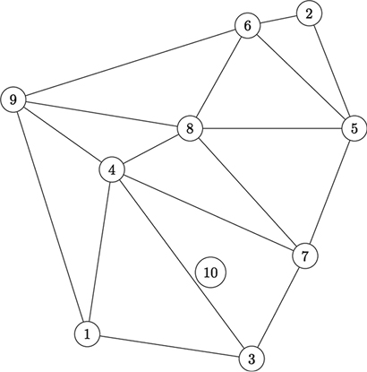
Figure 7-11: A 9-point DT with the 10th point we want to add

Figure 7-12: Three triangles in the DT have circumcircles containing point 10.
These triangles are no longer allowed to be in our DT, so we will remove them, yielding Figure 7-13.

Figure 7-13: We have removed the invalid triangles.
We haven’t finished yet. We need to fill in the hole that we’ve created and make sure that point 10 is properly connected to the other points. If we don’t, then we won’t have a collection of triangles, we’ll just have points and lines. The way we connect point 10 can be described simply: add an edge connecting point 10 to every vertex of the largest empty polygon that point 10 lies within (Figure 7-14).

Figure 7-14: Completing the 10-point DT by reconnecting valid triangles
Voilà! We started with a 9-point DT, added a new point, and now have a 10-point DT. This process may seem straightforward. Unfortunately, as is often the case with geometric algorithms, what seems clear and intuitive to the human eye can be tricky to write code for. But let’s not allow this to deter us, brave adventurers.
Implementing Delaunay Triangulations
Let’s start by assuming that we already have a DT, which we’ll call delaunay. It will be nothing more than a list of triangles. We can even start with one triangle alone:
delaunay = [points_to_triangle((0.2,0.8),(0.5,0.2),(0.8,0.7))]Next, we’ll define a point that we want to add to it, called point_to_add:
point_to_add = [0.5,0.5]We first need to determine which, if any, triangles in the existing DT are now invalid because their circumcircle contains the point_to_add. We’ll do the following:
- Use a loop to iterate over every triangle in the existing DT.
- For each triangle, find the circumcenter and radius of its circumcircle.
- Find the distance between the
point_to_addand this circumcenter. - If this distance is less than the circumradius, then the new point is inside the triangle’s circumcircle. We can then conclude this triangle is invalid and needs to be removed from the DT.
We can accomplish these steps with the following code snippet:
import math
invalid_triangles = []
delaunay_index = 0
while delaunay_index < len(delaunay):
    circumcenter,radius = triangle_to_circumcenter(delaunay[delaunay_index])
    new_distance = get_distance(circumcenter,point_to_add)
    if(new_distance < radius):
        invalid_triangles.append(delaunay[delaunay_index])
    delaunay_index += 1
This snippet creates an empty list called invalid_triangles, loops through every triangle in our existing DT, and checks whether a particular triangle is invalid. It does this by checking whether the distance between the point_to_add and the circumcenter is less than the circumcircle’s radius. If a triangle is invalid, we append it to the invalid_triangles list.
Now we have a list of invalid triangles. Since they are invalid, we want to remove them. Eventually, we’ll also need to add new triangles to our DT. To do that, it will help to have a list of every point that is in one of the invalid triangles, as those points will be in our new, valid triangles.
Our next code snippet removes all invalid triangles from our DT, and we also get a collection of the points that make them up.
points_in_invalid = []

for i in range(len(invalid_triangles)):
    delaunay.remove(invalid_triangles[i])
    for j in range(0,len(invalid_triangles[i])):
        points_in_invalid.append(invalid_triangles[i][j])

1 points_in_invalid = [list(x) for x in set(tuple(x) for x in points_in_invalid)]
We first create an empty list called points_in_invalid. Then, we loop through invalid_triangles, using Python’s remove() method to take each invalid triangle out of the existing DT. We then loop through every point in the triangle to add it to the points_in_invalid list. Finally, since we may have added some duplicate points to the points_in_invalid list, we’ll use a list comprehension 1 to re-create points_in_invalid with only unique values.
The final step in our algorithm is the trickiest one. We have to add new triangles to replace the invalid ones. Each new triangle will have the point_to_add as one of its points, and and two points from the existing DT as its other points. However, we can’t add every possible combination of point_to_add and two existing points.
In Figures 7-13 and 7-14, notice that the new triangles we needed to add were all triangles with point 10 as one of their points, and with edges selected from the empty polygon that contained point 10. This may seem simple enough after a visual check, but it’s not straightforward to write code for it.
We need to find a simple geometric rule that can be easily explained in Python’s hyper-literal style of interpretation. Think of the rules that could be used to generate the new triangles in Figure 7-14. As is common in mathematical situations, we could find multiple equivalent sets of rules. We could have rules related to points, since one definition of a triangle is a set of three points. We could have other rules related to lines, since another, equivalent definition of triangles is a set of three line segments. We could use any set of rules; we just want the one that will be the simplest to understand and implement in our code. One possible rule is that we should consider every possible combination of points in the invalid triangles with the point_to_add, but we should add one of those triangles only if the edge not containing the point_to_add occurs exactly once in the list of invalid triangles. This rule works because the edges that occur exactly once will be the edges of the outer polygon surrounding the new point (in Figure 7-13, the edges in question are the edges of the polygon connecting points 1, 4, 8, 7, and 3).
The following code implements this rule:
for i in range(len(points_in_invalid)):
    for j in range(i + 1,len(points_in_invalid)):
        #count the number of times both of these are in the bad triangles
        count_occurrences = 0
        for k in range(len(invalid_triangles)):
            count_occurrences += 1 * (points_in_invalid[i] in invalid_triangles[k]) *             (points_in_invalid[j] in invalid_triangles[k])
        if(count_occurrences == 1):
            delaunay.append(points_to_triangle(points_in_invalid[i], points_in_invalid[j], point_to_add))
Here we loop through every point in points_in_invalid. For each one, we loop through every following point in points_in_invalid. This double loop enables us to consider every combination of two points that was in an invalid triangle. For each combination, we loop through all the invalid triangles and count how many times those two points are together in an invalid triangle. If they are together in exactly one invalid triangle, then we conclude that they should be together in one of our new triangles, and we add a new triangle to our DT that consists of those two points together with our new point.
We have completed the steps that are required to add a new point to an existing DT. So we can take a DT that has n points, add a new point, and end up with a DT that has n + 1 points. Now, we need to learn to use this capability to take a set of n points and build a DT from scratch, from zero points all the way to n points. After we get the DT started, it’s really quite simple: we just need to loop through the process that goes from n points to n + 1 points over and over until we have added all of our points.
There is just one more complication. For reasons that we’ll discuss later, we want to add three more points to the collection of points whose DT we’re generating. These points will lie far outside our chosen points, which we can ensure by finding the uppermost and leftmost points, adding a new point that is higher and farther left than either of those, and doing similarly for the lowermost and rightmost points and the lowermost and leftmost points. We’ll se these points together as the first triangle of our DT. We’ll start with a DT that connects three points: the three points in the new triangle just mentioned. Then, we’ll follow the logic that we’ve already seen to turn a three-point DT into a four-point DT, then into a five-point DT, and so on until we’ve added all of our points.
In Listing 7-3, we can combine the code we wrote earlier to create a function called gen_delaunay(), which takes a set of points as its input and outputs a full DT.
def gen_delaunay(points):
    delaunay = [points_to_triangle([-5,-5],[-5,10],[10,-5])]
    number_of_points = 0


    while number_of_points < len(points): 1
        point_to_add = points[number_of_points]

        delaunay_index = 0

        invalid_triangles = [] 2
        while delaunay_index < len(delaunay):
            circumcenter,radius = triangle_to_circumcenter(delaunay[delaunay_index])
            new_distance = get_distance(circumcenter,point_to_add)
            if(new_distance < radius):
                invalid_triangles.append(delaunay[delaunay_index])
            delaunay_index += 1

        points_in_invalid = [] 3
        for i in range(0,len(invalid_triangles)):
            delaunay.remove(invalid_triangles[i])
            for j in range(0,len(invalid_triangles[i])):
                points_in_invalid.append(invalid_triangles[i][j])
        points_in_invalid = [list(x) for x in set(tuple(x) for x in points_in_invalid)]

        for i in range(0,len(points_in_invalid)): 4
            for j in range(i + 1,len(points_in_invalid)):
                #count the number of times both of these are in the bad triangles
                count_occurrences = 0
                for k in range(0,len(invalid_triangles)):
                    count_occurrences += 1 * (points_in_invalid[i] in invalid_triangles[k]) *                     (points_in_invalid[j] in invalid_triangles[k])
                if(count_occurrences == 1):
                    delaunay.append(points_to_triangle(points_in_invalid[i], points_in_invalid[j], point_to_add))

number_of_points += 1

    return(delaunay)
Listing 7-3: A function that takes a set of points and returns a Delaunay triangulation
The full DT generation function starts by adding the new outside triangle mentioned earlier. It then loops through every point in our collection of points 1. For every point, it creates a list of invalid triangles: every triangle that’s in the DT whose circumcircle includes the point we’re currently looking at 2. It removes those invalid triangles from the DT and creates a collection of points using each point that was in those invalid triangles 3. Then, using those points, it adds new triangles that follow the rules of Delaunay triangulations 4. It accomplishes this incrementally, using exactly the code that we have already introduced. Finally, it returns delaunay, a list containing the collection of triangles that constitutes our DT.
We can easily call this function to generate a DT for any collection of points. In the following code, we specify a number for N and generate N random points (x and y values). Then, we zip the x and y values, put them together into a list, pass them to our gen_delaunay() function, and get back a full, valid DT that we store in a variable called the_delaunay:
N=15
import numpy as np
np.random.seed(5201314)
xs = np.random.rand(N)
ys = np.random.rand(N)
points = zip(xs,ys)
listpoints = list(points)
the_delaunay = gen_delaunay(listpoints)
We’ll use the_delaunay in the next section to generate a Voronoi diagram.
From Delaunay to Voronoi
Now that we’ve completed our DT generation algorithm, the Voronoi diagram generation algorithm is within our grasp. We can turn a set of points into a Voronoi diagram by following this algorithm:
- Find the DT of a set of points.
- Take the circumcenter of every triangle in the DT.
- Draw lines connecting the circumcenters of all triangles in the DT that share an edge.
We already know how to do step 1 (we did it in the previous section), and we can accomplish step 2 withthe triangle_to_circumcenter() function. So the only thing we need is a code snippet that can accomplish step 3.
The code we write for step 3 will live in our plotting function. Remember that we pass a set of triangles and circumcenters to that function as its inputs. Our code will need to create a collection of lines connecting circumcenters. But it will not connect all of the circumcenters, only those from triangles that share an edge.
We’re storing our triangles as collections of points, not edges. But it’s still easy to check whether two of our triangles share an edge; we just check whether they share exactly two points. If they share only one point, then they have vertices that meet but no common edge. If they share three points, they are the same triangle and so will have the same circumcenter. Our code will loop through every triangle, and for each triangle, it will loop through every triangle again, and check the number of points that the two triangles share. If the number of common points is exactly two, then it will add a line between the circumcenters of the triangles in question. The lines between the circumcenters will be the boundaries of our Voronoi diagram. The following code snippet shows how we’ll loop through triangles, but it’s part of a larger plotting function, so don’t run it yet:
--snip--
for j in range(len(triangles)):
    commonpoints = 0
    for k in range(len(triangles[i])):
        for n in range(len(triangles[j])):
            if triangles[i][k] == triangles[j][n]:
               commonpoints += 1
    if commonpoints == 2:
        lines.append([list(centers[i][0]),list(centers[j][0])])
This code will be added to our plotting function, since our final goal is a plotted Voronoi diagram.
While we’re at it, we can make several other useful additions to our plotting function. The new plotting function is shown in Listing 7-4, with the changes in bold:
def plot_triangle_circum(triangles,centers,plotcircles,plotpoints, plottriangles,plotvoronoi,plotvpoints,thename):
    fig, ax = pl.subplots()
    ax.set_xlim([-0.1,1.1])
    ax.set_ylim([-0.1,1.1])

    lines=[]
    for i in range(0,len(triangles)):
        triangle = triangles[i]
        center = centers[i][0]
        radius = centers[i][1]
        itin = [0,1,2,0]
        thelines = genlines(triangle,itin)
        xs = [triangle[0][0],triangle[1][0],triangle[2][0]]
        ys = [triangle[0][1],triangle[1][1],triangle[2][1]]

        lc = mc.LineCollection(genlines(triangle,itin), linewidths=2)
        if(plottriangles):
            ax.add_collection(lc)
        if(plotpoints):
            pl.scatter(xs, ys)

        ax.margins(0.1)

     1 if(plotvpoints):
            pl.scatter(center[0],center[1])

        circle = pl.Circle(center, radius, color = 'b', fill = False)
        if(plotcircles):
            ax.add_artist(circle)

     2 if(plotvoronoi):
            for j in range(0,len(triangles)):
                commonpoints = 0
                for k in range(0,len(triangles[i])):
                    for n in range(0,len(triangles[j])):
                        if triangles[i][k] == triangles[j][n]:
                            commonpoints += 1
                if commonpoints == 2:
                    lines.append([list(centers[i][0]),list(centers[j][0])])

        lc = mc.LineCollection(lines, linewidths = 1)

        ax.add_collection(lc)

    pl.savefig(str(thename) + '.png')
    pl.close()
Listing 7-4: A function that plots triangles, circumcenters, circumcircles, Voronoi points, and Voronoi boundaries
First, we add new arguments that specify exactly what we want to plot. Remember that in this chapter we have worked with points, edges, triangles, circumcircles, circumcenters, DTs, and Voronoi boundaries. It could be overwhelming to the eye to plot all of these together, so we will add plotcircles to specify whether we want to plot our circumcircles, plotpoints to specify whether we want to plot our collection of points, plottriangles to specify whether we want to plot our DT, plotvoronoi to specify whether we want to plot our Voronoi diagram edges, and plotvpoints which to specify whether we want to plot our circumcenters (which are the vertices of the Voronoi diagram edges). The new additions are shown in bold. One addition plots the Voronoi vertices (circumcenters), if we have specified in our arguments that we want to plot them 1. The longer addition plots the Voronoi edges 2. We’ve also specified a few if statements that allow us to plot, or not plot, triangles, vertices, and circumcircles, as we prefer.
We’re almost ready to call this plotting function and see our final Voronoi diagram. However, first we need to get the circumcenters of every triangle in our DT. Luckily, this is very easy. We can create an empty list called circumcenters and append the circumcenter of every triangle in our DT to that list, as follows:
circumcenters = []
for i in range(0,len(the_delaunay)):
    circumcenters.append(triangle_to_circumcenter(the_delaunay[i]))
Finally, we’ll call our plotting function, specifying that we want it to draw the Voronoi boundaries:
plot_triangle_circum(the_delaunay,circumcenters,False,True,False,True,False,'final')Figure 7-15 shows our output.

Figure 7-15: A Voronoi diagram. Phew!
We’ve transformed a set of points into a Voronoi diagram in mere seconds. You can see that the boundaries in this Voronoi diagram run right up to the edge of the plot. If we increased the size of the plot, the Voronoi edges would continue even farther. Remember that Voronoi edges connect the centers of circumcircles of triangles in our DT. But our DT could be connecting very few points that are close together in the center of our plot, so all the circumcenters could lie within a small area in the middle of our plot. If that happened, the edges of our Voronoi diagram wouldn’t extend to the edges of the plot space. This is why we added the new outer triangle in the first line of our gen_delaunay() function; by having a triangle whose points are far outside our plot area, we can be confident that there will always be Voronoi edges that run to the edge of our map, so that (for example) we will know which post office to assign to deliver to new suburbs built on or outside the edge of the city.
Finally, you might enjoy playing with our plotting function. For example, if you set all of its input arguments to True, you can generate a messy but beautiful plot of all the elements we have discussed in this chapter:
plot_triangle_circum(the_delaunay,circumcenters,True,True,True,True,True,'everything')Our output is shown in Figure 7-16.
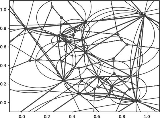
Figure 7-16: Magic eye
You can use this image to convince your roommates and family members that you are doing top-secret particle collision analysis work for CERN, or maybe you could use it to apply for an art fellowship as a spiritual successor to Piet Mondrian. As you look at this Voronoi diagram with its DT and circumcircles, you could imagine post offices, water pumps, crystal structures, or any other possible application of Voronoi diagrams. Or you could just imagine points, triangles, and lines and revel in the pure joys of geometry.
Summary
This chapter introduced methods for writing code to do geometric reasoning. We started by drawing simple points, lines, and triangles. We proceeded to discuss different ways to find the center of a triangle, and how this enables us to generate a Delaunay triangulation for any set of points. Finally, we went over simple steps for using a Delaunay triangulation to generate a Voronoi diagram, which can be used to solve the postmaster problem or to contribute to any of a variety of other applications. They are complex in some ways, but in the end they boil down to elementary manipulations of points, lines, and triangles.
In the next chapter, we discuss algorithms that can be used to work with languages. In particular, we’ll talk about how an algorithm can correct text that’s missing spaces and how to write a program that can predict what word should come next in a natural phrase.