
CHAPTER 6
Assessment of Model Adequacy
Model-based inferences depend completely on the fitted statistical model. For these inferences to be “valid” in any sense of the word, the fitted model must provide an adequate summary of the data upon which it is based. Hence a complete and thorough examination of model adequacy is just as important as careful model development.
The goal of statistical model development is to obtain the model that best describes the “middle” of the data. The specific definition of “middle” depends on the particular type of statistical model, but the idea is basically the same for all statistical models. In the normal errors linear regression model setting, we can describe the relationship between the observed outcome variable and one of the covariates with a scatterplot. This plot of points for two or more covariates is often described as the “cloud” of data. In model development, we find the regression surface (i.e., line, plane, or hyperplane) that best fits/splits the cloud. The notion of “best” in this setting means that we have equal distances from observed points to fitted points above and below the regression surface. A “generic” main effects model with some nominal covariates, which treats continuous covariates as linear, may not have enough tilts, bends, or turns to fit/split the cloud. Each step in the model development process is designed to tailor the regression surface to the observed cloud of data.
In most, if not all, applied settings, the results of the fitted model will be summarized for publication using point and interval estimates of clinically interpretable measures of the effect of covariates on the outcome. Examples of summary measures include the mean difference (for linear regression), the odds ratio (for logistic regression) and the hazard ratio (for proportional hazards regression). Because any summary measure is only as good as the model it is based on, it is vital that one evaluate how well the fitted regression surface describes the data cloud. This process is generally referred to as assessing the adequacy of the model’, like model development, it involves a number of steps. Performing these in a thorough and conscientious manner assures us that our inferential conclusions based on the fitted model are the best and most valid possible.
The methods for assessing the adequacy of a fitted proportional hazards model are essentially the same as for other regression models. We assume that the reader has had some experience with these methods, particularly with those for the logistic regression model [see Hosmer and Lemeshow (2000, Chapter 5)]. In the current setting, these include methods for: (1) examining and testing the proportional hazards assumption, (2) evaluating subject-specific diagnostic statistics that measure leverage and influence on the fit of the proportional hazards model and (3) computing summary measures of goodness-of-fit.
Central to the evaluation of model adequacy in any setting is an appropriate definition of a residual. As we discussed in Chapter 1, a regression analysis of survival time is set apart from other regression models, the fact that the outcome variable is time to an event and the observed values may be incomplete or censored. In earlier chapters, we suggested that the semiparametric proportional hazards model is a useful model for data of this type and we described why and how it may be fit using the partial likelihood. This combination of data, model and likelihood makes definition of a residual much more difficult than is the case in other settings.
Consider a logistic regression analysis of a binary outcome variable. In this setting, values of the outcome variable are “present” ( y = 1 ) or “absent” ( y = 0 ) for all subjects. The fitted model provides estimates of the probability that the outcome is present (i.e., the mean of Y). Thus, a natural definition of the residual is the difference between the observed value of the outcome variable and that predicted by the model. This form of the residual also follows as a natural consequence of characterizing the observed value of the outcome as the sum of a systematic component and an error component. The two key assumptions in this definition of a residual are: (1) the value of the outcome is known and (2) the fitted model provides an estimate of the “mean of the outcome variable.” Because assumption 2 and, more than likely, assumption 1 are not true when using the partial likelihood to fit the proportional hazards model to censored survival data, there is no obvious analog to the usual “observed minus predicted” residual used with other regression models.
The absence of an obvious residual has led to the development of several different residuals, each of which plays an important role in examining some aspect of a fitted proportional hazards model. Most software packages provide access to one or more of these residuals.
We assume, for the time being, that there are p covariates and that the n independent observations of time, covariates and censoring indicator are denoted by the triplet(ti, xi, ci), i = 1,2,...,n , where ci = 1 for uncensored observations and ci =0 otherwise. Schoenfeld (1982) proposed the first set of residuals for use with a fitted proportional hazards model and packages providing them refer to them as the “Schoenfeld residuals.” These are based on the individual contributions to the derivative of the log partial likelihood. This derivative for the kth co-variate is shown in (3.22) and is repeated here as
(6.1)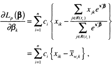
where
(6.2)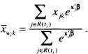
The estimator of the Schoenfeld residual for the ith subject on the kth covariate is obtained from (6.1) by substituting the partial likelihood estimator of the coefficient, ![]() , and is
, and is
(6.3)![]()
where
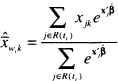
is the estimator of the risk set conditional mean of the covariate. Because the partial likelihood estimator of the coefficient, ![]() , is the solution to the equations obtained by setting (6.1) equal to zero, the sum of the Schoenfeld residuals is zero. The Schoenfeld residuals are equal to zero for all censored subjects and thus contain no information about the fit of the model. Hence, software packages set the value of the Schoenfeld residual to missing for subjects whose observed survival time is censored.
, is the solution to the equations obtained by setting (6.1) equal to zero, the sum of the Schoenfeld residuals is zero. The Schoenfeld residuals are equal to zero for all censored subjects and thus contain no information about the fit of the model. Hence, software packages set the value of the Schoenfeld residual to missing for subjects whose observed survival time is censored.
Grambsch and Therneau (1994) suggest that scaling the Schoenfeld residuals by an estimator of its variance yields a residual with greater diagnostic power than the unsealed residuals. Denote the vector of p Schoenfeld residuals for the ith subject as
![]()
where ![]() is the estimator in (6.3), with the convention that
is the estimator in (6.3), with the convention that ![]() = missing if ci0. Let the estimator of the p × p covariance matrix of the vector of residuals for the ith subject, as reported in Grambsch and Therneau (1994), be denoted by
= missing if ci0. Let the estimator of the p × p covariance matrix of the vector of residuals for the ith subject, as reported in Grambsch and Therneau (1994), be denoted by ![]() , and the estimator is missing if ci = 0. The vector of scaled Schoenfeld residuals is the product of the inverse of the covariance matrix times the vector of residuals, namely
, and the estimator is missing if ci = 0. The vector of scaled Schoenfeld residuals is the product of the inverse of the covariance matrix times the vector of residuals, namely
(6.4)![]()
The elements in the covariance matrix ![]() are, in the current setting, a weighted version of the usual sum-of-squares matrix computed using the data in the risk set. For the ith subject, the diagonal elements in this matrix are
are, in the current setting, a weighted version of the usual sum-of-squares matrix computed using the data in the risk set. For the ith subject, the diagonal elements in this matrix are
![]()
and the off-diagonal elements are
![]()
where

Grambsch and Therneau (1994) suggest using an easily computed approximation for the scaled Schoenfeld residuals. This suggestion is based on their experience that the matrix, ![]() , tends to be fairly constant over time. This occurs when the distribution of the covariate is similar in the various risk sets. Under this as-sumption, the inverse of
, tends to be fairly constant over time. This occurs when the distribution of the covariate is similar in the various risk sets. Under this as-sumption, the inverse of ![]() is easily approximated by multiplying the estimator of the covariance matrix of the estimated coefficients by the number of events (i.e., the observed number of uncensored survival times, m),
is easily approximated by multiplying the estimator of the covariance matrix of the estimated coefficients by the number of events (i.e., the observed number of uncensored survival times, m),
![]()
The approximate scaled Schoenfeld residuals are the ones computed by softvvar packages, namely
(6.5)![]()
Subsequent references to the scaled Schoenfeld residuals,![]() , will mean the approximation in (6.5), not the true scaled residuals in (6.4). We demonstrate the use of the scaled Schoenfeld residuals to assess the proportional hazards assumption in Section 6.3.
, will mean the approximation in (6.5), not the true scaled residuals in (6.4). We demonstrate the use of the scaled Schoenfeld residuals to assess the proportional hazards assumption in Section 6.3.
The next collection of residuals comes from the counting process formulation of a time-to-event regression model. This is an extremely useful and powerful mathematical tool for studying the proportional hazards model. However, most descriptions of it, including those in statistical software manuals, are difficult to understand without knowledge of calculus. In this section and those that follow, we try to present the counting process results in an intuitive and easily understood manner. An expanded introduction to the counting process approach is given in Appendix 2. A complete development of the theory as well as applications to other settings may be found in Fleming and Harrington (1991) and Andersen, Bor-gan, Gill and Keiding (1993).
Assume that we follow a single subject with covariates denoted by x from time “zero” and that the event of interest is death. We could use as the outcome any other event that can occur only once or the first occurrence of an event that can occur multiple times, such as cancer relapse. The counting process representation of the proportional hazards model is a linear-like model that “counts” whether the event occurs (e.g., the subject dies) at time t. The basic model is
(6.6)![]()
where the function N(t) is the “count” that represents the observed part of the model, the function ![]() (t,x,β) is the “systematic component” of the model, and the function M (t) is the “ error component. ”
(t,x,β) is the “systematic component” of the model, and the function M (t) is the “ error component. ”
The function N(t) is defined to be equal to zero until the exact time the event occurs and is equal to one thereafter. If the total length of follow-up is one year, and our subject dies on day 200, then
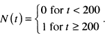
If the subject does not die during the one year of follow-up, then the count is always zero, N(t) - 0 . Hence, the maximum value of the count function occurs at the end of follow-up of the subject and is equal to the value of the censoring indicator variable.
The systematic component of the model is, as we show in Appendix 2, equal to the cumulative hazard at time t under the proportional hazards model,
![]()
until follow-up ends on the subject, and it is equal to zero thereafter. Thus, the value of the function for a subject who either dies or is censored on day 200 is
![]()
where H0(t) is the cumulative baseline hazard function. It follows that the maximum value for the systematic component also occurs at the end of follow-up, regardless of whether the event occurred. The function M(t) in (6.6) is, under suitable mathematical assumptions, a martingale and plays the role of the error component. It has many of the same properties that error components in other models have, in particular its mean is zero under the correct model. If we rearrange (6.6), M (t) may be expressed in the form of a “residual” as
(6.7)![]()
The quantity in (6.7) is called the martingale residual. In theory, it has a value at each time r, but the most useful choice of time at which to compute the residual is the end of follow-up, yielding a value for the ith subject of
(6.8)![]()
because ![]() (ti,x,β) = H(ti,x,β). For ease of notation, let Mi, = M(ti). The estimator, obtained by substituting the value of the partial likelihood estimator of the coefficients,
(ti,x,β) = H(ti,x,β). For ease of notation, let Mi, = M(ti). The estimator, obtained by substituting the value of the partial likelihood estimator of the coefficients, ![]() is
is
(6.9)![]()
since N(ti) = ci and the estimator ![]() is defined in (3.42). We mentioned in Chapter 5 that this residual, (6.9), can be used for a graphical method to assess the scale of a continuous covariate. We use the martingale residuals in Section 6.5 to provide a tabular display of model fit.
is defined in (3.42). We mentioned in Chapter 5 that this residual, (6.9), can be used for a graphical method to assess the scale of a continuous covariate. We use the martingale residuals in Section 6.5 to provide a tabular display of model fit.
The residual in (6.9) is also called the Cox–Snell or modified Cox–Snell residual (see Cox and Snell (1968) and Collett (2003)). This terminology is due to the work of Cox and Snell, who showed that the values of ![]() may be thought of as observations from a censored sample with an exponential distribution and parameter equal to 1.0. In our experience, this distribution theory is not as useful for model evaluation as the theory derived from the counting process approach.
may be thought of as observations from a censored sample with an exponential distribution and parameter equal to 1.0. In our experience, this distribution theory is not as useful for model evaluation as the theory derived from the counting process approach.
Using the counting process approach, the expressions in (6.7) and (6.8) are a completely natural way to define a residual. To see why it also makes sense to consider (6.8) as a residual in the proportional hazards regression model, assume for ease of notation, that there are no ties and that the value of the baseline hazard at time ti is
(6.10)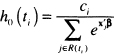
and that the cumulative baseline hazard is
(6.11)![]()
The Breslow estimator of the cumulative baseline hazard is obtained from (6.11) by substituting the value of the partial likelihood estimator of the coefficients, ![]() . Under these assumptions, the derivative in (6.11) may be expressed as
. Under these assumptions, the derivative in (6.11) may be expressed as
(6.12)![]()
The expression in (6.12) is similar to likelihood equations obtained for other models, such as linear and logistic regression, in that it expresses the partial derivative as a sum of the value of the covariate times an “observed minus expected” residual.
The next set of residuals are obtained by expressing the martingale residuals, (6.12), in a slightly different form. The score equation for the ith covariate may be expressed as
(6.13)![]()
The expression for Lik is somewhat complex. Readers who are willing to accept without further elaboration that the estimator of Lik is the score residual provided by software packages may skip the next paragraph where we describe Lik in greater detail.
The score residual for the ith subject on the kth covariate in (6.13) may be expressed as
(6.14)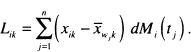
The mean in the expression, ![]() , is the value of (6.2) computed at tj. The quantity dMi(tj) is the change in the martingale residual for the ith subject at time tjand is
, is the value of (6.2) computed at tj. The quantity dMi(tj) is the change in the martingale residual for the ith subject at time tjand is
(6.15)![]()
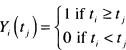
The first part of (6.15), dNi(tj), is the change in the count function for the ith subject at timer,. This will always be equal to zero for censored subjects. For uncensored subjects, it will be equal to zero except at the actual observed survival time, when it will be equal to one. That is, dNi(ti) = 1 for uncensored subjects, in the second part of (6.15), the function Yi(tj) is called the at risk process and is defined as follows:
and h0(tj) is the value of (6.10) evaluated at tj An expanded computational formula yields the estimator
(6.16)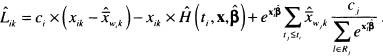
Let the vector of p score residuals for the ith subject be denoted as
(6.17)![]()
A scaled version of the score residuals in (6.17) is also used in model evaluation. These are defined as
(6.18)![]()
where ![]() is the estimator of the covariance matrix of the estimated coefficients. These are commonly referred to as the scaled score residuals and their values may be obtained from some software packages. We use the score and scaled score residuals to measure the leverage and influence, respectively, of particular subjects.
is the estimator of the covariance matrix of the estimated coefficients. These are commonly referred to as the scaled score residuals and their values may be obtained from some software packages. We use the score and scaled score residuals to measure the leverage and influence, respectively, of particular subjects.
Before moving on, we provide a brief summary of residuals. The martingale residual, ![]() , in (6.9) has the form typically expected of a residual in that it resembles the difference between an observed outcome and a predicted outcome. The other four residuals (Schoenfeld, scaled Schoenfeld, score, and scaled score) are covariate-specific. Every subject has a value of the score residual for the ith covariate,
, in (6.9) has the form typically expected of a residual in that it resembles the difference between an observed outcome and a predicted outcome. The other four residuals (Schoenfeld, scaled Schoenfeld, score, and scaled score) are covariate-specific. Every subject has a value of the score residual for the ith covariate, ![]() in (6.16) and for the scaled score residual,
in (6.16) and for the scaled score residual, ![]() from (6.18), but the Schoenfeld residual in (6.3) and the scaled Schoenfeld residual in (6.5) are defined only at the observed survival times. Thus, there are only m subjects with values for these residuals. Each of these residuals provides a useful tool for examining one or more aspects of model adequacy.
from (6.18), but the Schoenfeld residual in (6.3) and the scaled Schoenfeld residual in (6.5) are defined only at the observed survival times. Thus, there are only m subjects with values for these residuals. Each of these residuals provides a useful tool for examining one or more aspects of model adequacy.
Next we consider methods for assessing the proportional hazards assumption.
6.3 ASSESSING THE PROPORTIONAL HAZARDS ASSUMPTION
The proportional hazards assumption is vital to the interpretation and use of a fitted proportional hazards model. As discussed in detail in Chapter 4, the estimated hazard ratios do not depend on time. Specifically, the proportional hazards model has a log-hazard function of the form
(6.19)![]()
This function has two parts, the log of the baseline hazard function, ln[h0(t)], and the linear predictor, x′β . Methods for building the linear predictor part of the model are discussed in detail in Chapter 5. The proportional hazards assumption characterizes the model as a function of time, not of the covariates per se. Assume for the moment that the model contains a single dichotomous covariate. A plot of the log-hazard, (6.19), over time would produce two continuous curves, one forx = 0, ln[h0(t)], and the other for x = 1, ln[h0(t)] +β. It follows that the difference between these two curves at any point in time is β, regardless of how simple or complicated the baseline hazard function is. This is the reason the estimated hazard ratio, ![]() , has such a simple and useful interpretation.
, has such a simple and useful interpretation.
As a second example, suppose age is the only covariate in the model and that it is scaled linearly. Consider the plots over time of the log-hazard function for age a and age a + 10. If the coefficient, β, is positive, then the difference between the two plotted functions is 10β at every point in time. Assessing the proportional hazards assumption is an examination of the extent to which the two plotted hazard functions are equidistant from each other over time.
There are, effectively, an infinite number of ways the model in (6.19) can be changed to yield non-proportional hazard functions or log-hazard functions that are not equidistant over time. As a result, a large number of tests and procedures have been proposed. However, work by Grambsch and Therneau (1994) and simulations by Ng’andu (1997) show that one easily performed test and an associated graph yield an effective method for examining this critical assumption.
Grambsch and Therneau (1994) consider an alternative to the model in (6.19) originally proposed by Schoenfeld (1982), that allows the effect of the covariate to change over time as follows:
(6.20)![]()
where gj(t) specified function of time. The rationale for this model is that the effect of a covariate could change continuously or discretely over the period of follow-up. For example, the baseline value of a specific covariate may lose its relevance over time. The opposite could also occur, namely the baseline measure is more strongly associated with survival later in the follow-up. Under the model in (6.20), Grambsch and Therneau show that the scaled Schoenfeld residuals in (6.4), and their approximation in (6.5), have, for theyth covariate, a mean at time t of approximately
(6.21)![]()
The result in (6.21) suggests that a plot of the scaled Schoenfeld residuals over time may be used to assess visually whether the coefficient γj is equal to zero and, if not, what the nature of the time dependence, gj(t), may be. Grambsch and Therneau derive a generalized least-squares estimator of the coefficients and a score test of the hypothesis that they are equal to zero, given specific choices for the functions gj(t). In addition, they show that specific choices for the function yield previously proposed tests. For example, using g(t) = ln(t) yields a model first suggested by Cox (1972) and a test by Gill and Schumacher (1987) discussed by Chappell (1992). With this function, the model in (6.20) is
![]()
and the linear predictor portion of the model in (6.20) is
(6.22)![]()
The form of the linear predictor in (6.22) suggests that we can test the hypothesis that γj = 0 via the partial likelihood ratio test, score test, or Wald test obtained when the time varying interaction xj ln(t) is added to the proportional hazards model. The advantage of this approach over the generalized least-squares score test proposed by Grambsch and Therneau is that it may be done using the model fitting software in many statistical software packages. One should note that when the interaction term, xj In(t), is included in the model, the partial likelihood becomes much more complicated. The interaction is a function of follow up time, its value must be recomputed for each term in the risk set at each observed survival time. The interaction term is not simply the product of the covariate and the subject’s observed value of time, xj In(tj).
Other functions of time have been suggested, for example Quantin et al. (1996) suggest using g(t) = ln[H0(t)]. Based on simulations reported in their paper, this test appears to have good power, but it is not as easy to compute as the test based on g(t) = ln(t). Because the Breslow estimator of H0 (t) must be computed and must be accessible at each observed survival time. The STATA package allows us to use, in addition to g(t) = ln(t), the functions g(t) = t, g(t) = ![]() KM(t) and g(t) = rank(t). Simulations in Quantin et al. (1996) and Ng’andu (1997), show that the test based on g(t) = ln(t) has power nearly as high or higher than other commonly used functions to detect reasonable alternatives to proportional hazards. While this is generally true, our experience is that, in specific cases, the significance level of the tests may vary with the function from highly significant with one choice to marginal or non-significant with another choice. For this reason, we tend to perform the tests with a variety of functions. Using more than one test certainly increases the chance of making a Type I error for each covariate, but finding a “significant” time varying effect may lead to a more informative model. In any case, if the test for any covariate is significant, then its time varying effect must make clinical sense.
KM(t) and g(t) = rank(t). Simulations in Quantin et al. (1996) and Ng’andu (1997), show that the test based on g(t) = ln(t) has power nearly as high or higher than other commonly used functions to detect reasonable alternatives to proportional hazards. While this is generally true, our experience is that, in specific cases, the significance level of the tests may vary with the function from highly significant with one choice to marginal or non-significant with another choice. For this reason, we tend to perform the tests with a variety of functions. Using more than one test certainly increases the chance of making a Type I error for each covariate, but finding a “significant” time varying effect may lead to a more informative model. In any case, if the test for any covariate is significant, then its time varying effect must make clinical sense.
In most settings, we recommend the following two-step procedure for assessing the proportional hazards assumption: (1) calculate covariate specific tests and (2) plot the scaled and smoothed scaled Schoenfeld residuals obtained from the model. The results of the two steps should support each other. Methods for handling nonproportional hazards are discussed in Chapter 7, where we consider extensions of the proportional hazards model.
Table 6.1 Score Tests and p-values for Proportional Hazards for Each of the Covariates as Well as the Global Test for the Model in Table 5.13 Fit to the WHAS500 Data
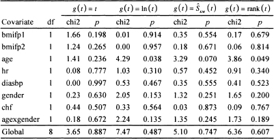
We now turn to evaluating the model developed in Chapter 5 for the WHAS500 data, shown in Table 5.13. This model is relatively complex in that it contains 8 terms: three main effects without interactions, an interaction and its main effects, and two terms that model nonlinear effects of a continuous covariate. Our first step is to evaluate the score test based on the scaled Schoenfeld residuals using each of the four functions of time available in STATA. The results are shown in Table 6.1.
The results in Table 6.1 indicate that there is some evidence, for three of the four functions of time, of the hazard being nonproportional in age. Nevertheless, the evidence for this is weak. Age is involved in an interaction with gender, which does not have a significant score test. If the evidence were stronger, this would have implied that the nonproportional hazard in age may be for males in the multi-variable model because the main effect for age corresponds to the age effect for males (gender = 0). The global 8 degrees-of-freedom tests are not significant. We also point out the importance of using the covariate specific tests because, if we do not, we might miss a possible non-proportionality in any of the individual covariates. There is no strong evidence of nonproportional hazards for any of the terms in the model. We obtained similar results when we added time varying interactions of the form g(t)*x to the model and assessed significance using Wald statistics for individual terms and the partial likelihood ratio test for the global test of proportional hazards. At this point, it makes sense to look at a scatterplot of the scaled Schoenfeld residuals to see whether they support the results of the score tests.
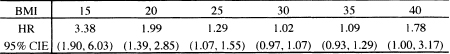
It is our experience that these plots are difficult to interpret, as any departure from proportional hazards may be subtle and difficult to see, even with a smooth added to the plot. Rather than begin with age, we illustrate the plot for heart rate (hr) in Figure 6.1 to provide an example of what the plot should look like for a continuous covariate when the score test fails to reject the null hypothesis of no time varying effect [i.e., H0:γj.= 0 in (6.21)|.
Figure 6.1 Scatterplot of scaled Schoenfeld residuals for heart rate and their lowess smooth versus the natural log of follow up time (years), follow up time, the Kaplan-Meier estimate, and the rank of follow up time.
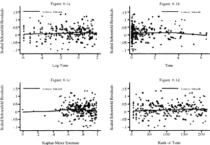
In Figure 6.1, we plot the scaled Schoenfeld residuals versus each of the four functions of time used in Table 6.1. In Figure 6.1a we plot versus log of time. This plot emphasizes the first year of follow up, as 75 percent of the plot is devoted to this time interval. This plot shows no discernable pattern, appearing to be “randomly” scattered about zero. The lowess smooth has a slight positive slope. The slight downturn at the far right is likely due to the effect of the two small values in the lower right of the plot. In Figure 6.1b, the scaled Schoenfeld residuals are plotted versus follow up time. About 75 percent of the plot is devoted to the time interval from one to six years. This plot places a high visual emphasis on a few subjects with follow up times that exceed three years. In particular, we see that the downturn in the far right of Figure 6.1b is much more visible and likely due to the effect on the lowess smooth of the subjects with the four longest follow up times. Overall the lowess smooth displays a slight rise and then fall, which by the score test is not a significant departure from a slope of zero. In Figure 6. lc, the scaled Schoenfeld residuals are plotted versus the Kaplan-Meier estimate of the survival function. The plot places undue emphasis on the four subjects with the longest follow up times (i.e., Kaplan-Meier estimates < .4). In the remainder of the plot, to the right of 0.4, the points appear to be randomly scattered about the lowess smooth, which appears to have a slope equal to zero. In this case, a better plot would be one over the interval [0.4, 1], which we leave as an exercise. The scaled Schoenfeld residuals are plotted in Figure 6.Id versus the rank of survival time in the sample of 500. The plot looks similar to Figure 6.1c, but with better resolution for shorter follow up times (i.e., ones with rank < 100). Like the other three plots, there is no obvious departure from the points being randomly distributed about the lowess smooth, which has a slight bend. In summary, the four plots support the proportional hazards assumption.
Figure 6.2 Scatterplot of scaled Schoenfeld residuals for congestive heart complications and their lowess smooth versus the natural log of follow up time (years), follow up time, the Kaplan-Meier estimate, and the rank of follow up time.
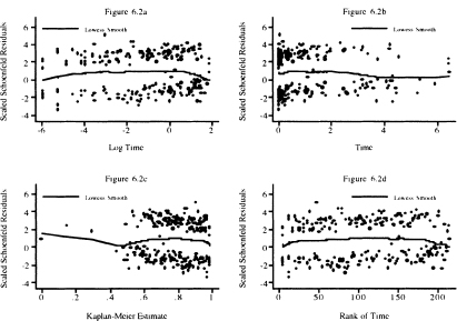
Next we examine the same four scatterplots of the scaled Schoenfeld residuals for congestive heart complications (chf) in Figure 6.2. Congestive heart complications is a dichotomous covariate and each of the four score tests fails to reject the hypothesis of proportional hazards. We first note the two bands of points. The upper band corresponds to the 110 subjects who had complications and subsequently died. The points in the lower band correspond to the 105 subjects with no complications who died. This band-like behavior is typical of the scaled score residuals for dichotomous covariates that appear in the model as a main effect only. When dichotomous covariates are involved in an interaction with a continuous covariate, the scatterplot of the scaled score residuals for the main effect and its interaction tend to look more like those of a fully continuous covariate.
The lowess smooth in Figure 6.2a has a vaguely parabolic shape in that it rises, levels, and then drops. The rise occurs during the first seven days, 6.69 = 365 × exp(–4). The lowess smooth has slope about zero from 7 days to one year, 0 = ln(1), and then drops. The overall effect is that a straight line would have slope zero. It is not clear at this point if the early and late departures from zero slope are meaningful so, for the time being, we proceed as if the plot supports the score tests. The other three plots display these trends, but, as noted above in the discussion of Figure 6.1, with a focus on different intervals of follow up time. However, we return to this point and explore the possibility of a time varying effect in more detail in Chapter 7 where we discuss time varying covariates.
The scatterplots and lowess smooths of the scaled Schoenfeld residuals for the two fractional polynomial transformations of body mass index (bmifpl and bmifp2), diastolic blood pressure (diasbp), gender, and the gender by age interaction support the score test results. Hence we proceed, treating the hazard in these covariates as being proportional.
Figure 6.3 Scatterplot of scaled Schoenfeld residuals for age and their lowess smooth versus the natural log of follow up time (years), follow up time, the Kaplan-Meier estimate, and the rank of follow up time.
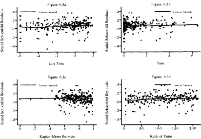
Next we show, in Figure 6.3, four scatterplots of the scaled Schoenfeld residuals and their lowess smooth for age. In Figure 6.3a, we see that the lowess smooth has slope zero for the first week of follow up; from this point on, the trend is slightly upward. The upward trend is easier to see in Figure 6.1b and Figure 6.Id. As we noted above, due to the inclusion of the age-by-gender interaction, we believe that non-proportionality may be among males only. As with the case of congestive heart complications, we are going to proceed with further model evaluation assuming that the main effect age has a proportional hazard, returning to reexamine the issue in Chapter 7.
In closing, we note two points: (1) The score tests and scatterplots based on the scaled Schoenfeld residuals with various functions of follow up time are the primary diagnostic test and descriptive statistics for assessing whether the hazard is proportional in each covariate separately as well as overall, and (2) Application of the tests and plots, in general, supports treating the model in Table 5.13 as adhering to the proportional hazards assumption.
6.4 IDENTIFICATION OF INFLUENTIAL AND POORLY FIT SUBJECTS
Another important aspect of model evaluation is a thorough examination of regression diagnostic statistics to identify which, if any, subjects: (1) have an unusual configuration of covariates, (2) exert an undue influence on the estimates of the parameters, and/or (3) have an undue influence on the fit of the model. Statistics similar to those used in linear and logistic regression are available to perform these tasks with a fitted proportional hazards model. There are some differences in the types of statistics used in linear and logistic regression and proportional hazards regression, but the essential ideas are the same in all three settings.
Leverage is a diagnostic statistic that measures how “unusual” the values of the covariates are for an individual. In some sense it is a residual in the covariates. In linear and logistic regression, leverage is calculated as the distance of the value of the covariates for a subject to the overall mean of the covariates [see Hosmer and Lemeshow (2000), Kleinbaum, Kupper, Muller and Nizam (1998), and Ryan (1997)). It is proportional to ![]() . The leverage values in these settings have nice properties in that they are always positive and sum over the sample to the number of parameters in the model. While it is technically possible to break the leverage into values for each covariate, this is rarely done in linear and logistic regression. Leverage is not quite so easily defined nor does it have the same nice properties in proportional hazards regression. This is due to the fact that subjects may appear in multiple risk sets and thus may be present in multiple terms in the partial likelihood.
. The leverage values in these settings have nice properties in that they are always positive and sum over the sample to the number of parameters in the model. While it is technically possible to break the leverage into values for each covariate, this is rarely done in linear and logistic regression. Leverage is not quite so easily defined nor does it have the same nice properties in proportional hazards regression. This is due to the fact that subjects may appear in multiple risk sets and thus may be present in multiple terms in the partial likelihood.
The score residuals defined in (6.16) and (6.17) form the nucleus of the proportional hazards diagnostics. The score residual for the ith subject on the kth covariate, see (6.14), is a weighted average of the distance of the value, xjk, to the risk set means, ![]() , where the weights are the change in the martingale residual, dMi (tj). The net effect is that, for continuous covariates, the score residuals have the linear regression leverage property that the further the value is from the mean, the larger the score residual is, but “large” may be either positive or negative. Thus, the score residuals are sometimes referred to as the leverage or partial leverage residuals.
, where the weights are the change in the martingale residual, dMi (tj). The net effect is that, for continuous covariates, the score residuals have the linear regression leverage property that the further the value is from the mean, the larger the score residual is, but “large” may be either positive or negative. Thus, the score residuals are sometimes referred to as the leverage or partial leverage residuals.
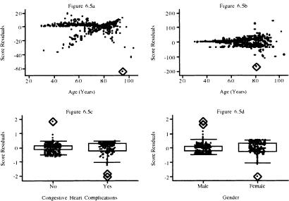
The graphs of the score residuals for the covariates bmifpl, bmifp2, heart rate, and diastolic blood pressure obtained from the fitted model in Table 5.13 are shown in Figure 6.4a to Figure 6.4d. These four terms were chosen because they are continuous variables and not involved in an interaction in the fitted model. The graphs for remaining model terms are in Figure 6.5a to Figure 6.5d.
To aid in the interpretation of the plots in this section, we have used the diamond to highlight the points that we feel lie further from the remainder of the data than we would expect. These represent subjects whose data we will want to investigate further.
In Figure 6.4, we observe three extreme points for body mass index, one for heart rate and two for diastolic blood pressure. In Figure 6.5, we see one extreme point for age and one for the age-by-gender interaction. For dichotomous covariates, it is more informative to use a box plot at each level of the covariate. In the plot for congestive heart complications, we see one for chf = 0 and two for chf = 1. In the plot for gender, there are two values for male and one for female that warrant further attention.
In linear and logistic regression, high leverage is not necessarily about a concern. However, a subject with a high value for leverage may contribute undue influence to the estimate of a coefficient. The same is true in proportional hazards regression. To examine influence in the proportional hazards setting, we need statistics analogous to Cook’s distance in linear and logistic regression. The purpose of Cook’s distance is to obtain an easily computed statistic that approximates the change in the value of the estimated coefficients if a subject is deleted from the data. This is denoted as
(6.23)![]()
where ![]() k denotes the partial likelihood estimator of the coefficient computed using the entire sample of size n and
k denotes the partial likelihood estimator of the coefficient computed using the entire sample of size n and ![]() denotes the value of the estimator if the ith subject is removed. Cain and Lange (1984) show that an approximate estimator of (6.23) is the kth element of the vector of coefficient changes
denotes the value of the estimator if the ith subject is removed. Cain and Lange (1984) show that an approximate estimator of (6.23) is the kth element of the vector of coefficient changes
(6.24)![]()
Figure 6.4 Graphs of the score residuals computed from the model in Table 5.13 for (a) bmifpl, (b) bmifp2, (c) heart rate, and (d) diastolic blood pressure.
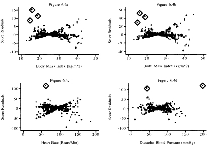
Figure 6.5 Graphs of the score residuals computed from the model in Table 5.13 for (a) age, (b) age by gender interaction, (c) congestive heart complications, and (d) gender.
where ![]() , is the vector of score residuals, (6.17), and
, is the vector of score residuals, (6.17), and ![]() is the estimator of the covariance matrix of the estimated coefficients. These are commonly referred to as the scaled score residuals and their values may be obtained from some software packages, for example, SAS, and easily computed in STATA.
is the estimator of the covariance matrix of the estimated coefficients. These are commonly referred to as the scaled score residuals and their values may be obtained from some software packages, for example, SAS, and easily computed in STATA.
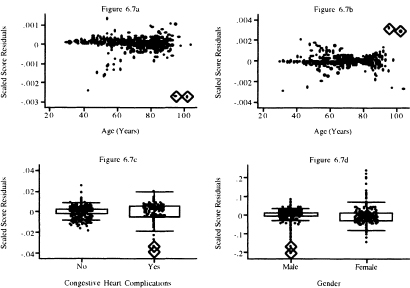
Graphs of the scaled score residuals, (6.24), are presented in Figure 6.6 for the covariates whose score residuals are graphed in Figure 6.4. and in Figure 6.7 for the variables whose score residuals are plotted in Figure 6.5. The plots in Figures 6.4 and 6.6 look different. Nevertheless, the same three points are identified as being influential for bmifpl in Figures 6.4a and Figure 6.6a. However, it appears that three different points are identified as being influential for bmifp2. Similarly, we see a single influential point in the plots for heart rate and diastolic blood pressure.
In Figure 6.7 we see two points that may have influence on the coefficient for age and two points for the interaction of age and gender. The box plot for congestive heart complications shows two possibly influential subjects with chf = 1. The plot for gender identifies perhaps three male subjects with influence. Note that two male subjects with very small influence values that are so close together they are indistinguishable on the graph.
Cook’s distance in linear and logistic regression may be used to provide a single overall summary statistic of the influence a subject has on the estimators of
Figure 6.6 Graphs of the scaled score residuals computed from the model in Table 5.13 for (a) bmifpl, (b) bmifp2, (c) heart rate, and (d) diastolic blood pressure.
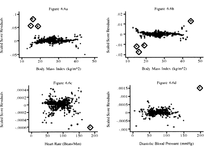
Figure 6.7 Graphs of the scaled score residuals computed from the model in Table 5.13 for (a) age, (b) age-by-gender interaction, (c) congestive heart complications, and (d) gender.
all the coefficients. The overall measure of influence is
![]()
and using (6.24) it may be approximated using
so
(6.25)![]()
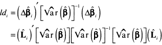
The statistic in (6.25) has been shown by Pettitt and Bin Daud (1989) to be an approximation to the amount of change in the log partial likelihood when the ith subject is deleted. In this context, the statistic is called the likelihood displacement statistic, hence the rationale for labeling it ld in (6.25), thus
(6.26)![]()
We feel it makes the most sense to plot ldi in (6.25) versus the martingale residuals.
The plots of the values of the likelihood displacement statistic versus the martingale residuals are shown in Figure 6.8. The plot has an asymmetric “cup” shape with the bottom of the cup at zero. In linear and logistic regression, the influence diagnostic, Cook’s distance, is a product of a residual measure and leverage. While the same concise representation does not hold in proportional hazards regression, it is approximately true in the sense that an influential subject will have a large residual and/or leverage. Thus, the largest values of the likelihood displacement form the sides of the cup and correspond to poorly fit subjects (ones with either large negative or large positive martingale residuals).
The next step in the modeling process is to identify explicitly the subjects with the extreme values, refit the model deleting these subjects, and calculate the change in the individual coefficients. The final decision on the continued use of a subject’s data to fit the model will depend on the observed percentage change in the coefficients that results from deleting the subject’s data and, more importantly, the clinical plausibility of that subject’s data.
By examining the values of the covariates and diagnostic statistics, we find 10 subjects with high leverage, high influence or large Cook’s distance. These subjects are listed, with their data, in Table 6.2. The subjects are generally older, with low body mass index. At this stage of the analysis, we do nothing, delaying further action until we examine influence on parameter estimates.
Table 6.2 Nine Subjects with High Leverage, High Influence or Large Cook’s Distance from the Fitted Model in Table 5.13
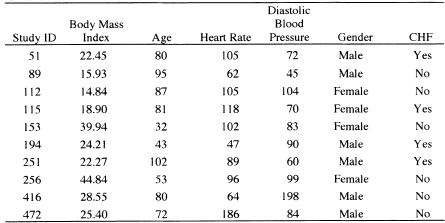
We leave it as an exercise to verify that, when we fit the model in Table 5.13, deleting the 10 subjects listed in Table 6.2, the percentage change in the eight estimated coefficients is 33.7, 31.2, 14.9, 17.7, 19.9, 11.2, 2.8, and 14.7, respectively. The greatest effect of the deletion is on the coefficients for the two fractional polynomial variables for body mass index. The change is largely due to deletion of subjects 89, 112, 115, and 256. This is not unexpected because these four subjects are among those with the lowest and highest values of bmi. The changes in the other coefficients are less than 20 percent, though the change in the estimate of the coefficient for diastolic blood pressure is 19.9 percent.
We consulted with the Worcester Heart Attack Study team on the plausibility of the data for subjects 89, 11, 115, 256, and 416. The bmi values for subjects influential for the estimates of the coefficients (89, 112, 115 and 256) for the two fractional polynomial variables were judged to be reasonable and should be kept in the analysis. However, they felt that a diastolic blood pressure of 198, while clinically possible, was so unusual relative to the other subjects in the study that this subject should be removed from the analysis.
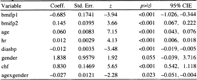
As a result of the deletion, we fit the model in Table 5.13 after deleting subject 416, and the results are displayed in Table 6.3. Other than a change in the estimated coefficient for diastolic blood pressure by about 15 percent, all other model summary statistics are essentially unchanged. The results of model evaluation were also essentially unchanged.
Figure 6.8 Graphs of the likelihood displacement or Cook’s distance statistic computed from the model in Table 5.13 versus the martingale residual.
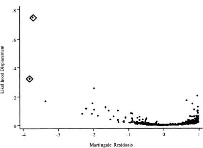
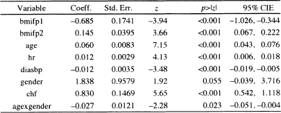
Table 6.3 Estimated Coefficients, Standard Errors, z-Scores, Two-Tailed p-values, and 95% Confidence Interval Estimates for the Preliminary Final Proportional Hazards Model for the WHAS500 data, n = 499
In summary, we feel it is important to examine plots of the score residuals, scaled score residuals, and the likelihood displacement statistic. The first two statistics are useful for identifying subjects with high leverage or who influence the value of a single coefficient. The latter provides useful information for assessing influence on the vector of coefficients. Each statistic portrays an important aspect of the effect a particular subject has on the fitted model. One always hopes that major problems are not uncovered. However, if the model does display abnormal sensitivity to the subjects deleted, this is a clear indication of fundamental problems in the model and we recommend going back to “square-one” and repeating each step in the modeling process, perhaps with these subjects deleted. The next step in the modeling process is to compute an overall goodness-of-fit test.
6.5 ASSESSING OVERALL GOODNESS-OF-FIT
Until quite recently, all the proposed tests for the overall goodness-of-fit of a proportional hazards model were difficult to compute in most software packages. For example, the test proposed by Schoenfeld (1980) compares the observed number of events with a proportional hazards regression model-based estimate of the expected number of events in each of G groups formed by partitioning the time axis and covariate space. Unfortunately, the covariance matrix required to form a test statistic comparing the observed to expected number of events is quite complex to compute. The test proposed by Lin, Wei and Ying (1993) is based on the maximum absolute value of partial sums of martingale residuals. This test requires complex and time-consuming simulations to obtain a significance level. Other tests [e.g., O’Quigley and Pessione (1989) and Pettitt and Bin Daud (1990)| require that the time axis be partitioned and interactions between covariates and interval-specific, time-dependent covariates be added to the model. Overall goodness-of-fit is based on a significance test of the coefficients for the added variables.
Grønnesby and Borgan (1996) propose a test similar to the Hosmer-Lemeshovv test |Hosmer and Lemeshow (2000) | used in logistic regression. They suggest partitioning the data into G groups based on the ranked values of the estimated risk score, x′![]() . The test is based on the sum of the martingale residuals within each group, and it compares the observed number of events in each group to the model-based estimate of the expected number of events. Using the counting process approach, they derive an expression for the covariance matrix of the vector of G sums. They show that their quadratic form test statistic has a chi-square distribution with G –1 degrees of freedom when the fitted model is the correct model and the sample is large enough that the estimated expected number of events in each group is large. As presented in their paper, the calculations of Gr0nnesby and Borgan (1996) are not a trivial matter.
. The test is based on the sum of the martingale residuals within each group, and it compares the observed number of events in each group to the model-based estimate of the expected number of events. Using the counting process approach, they derive an expression for the covariance matrix of the vector of G sums. They show that their quadratic form test statistic has a chi-square distribution with G –1 degrees of freedom when the fitted model is the correct model and the sample is large enough that the estimated expected number of events in each group is large. As presented in their paper, the calculations of Gr0nnesby and Borgan (1996) are not a trivial matter.
May and Hosmer (1998), following the method used by Tsiatis (1980) to derive a goodness-of-fit test in logistic regression, prove that Gr0nnesby and Borgan’s test is the score test for the addition of G–1 design variables, based on the G groups, to the fitted proportional hazards model. Thus, the test statistic may be calculated in any package that performs score tests. Using the asymptotic equivalence of score tests and likelihood ratio tests, one may approximate the score test with the partial likelihood ratio test, which may be done in any package.
One may be tempted to define groups based on the subject-specific estimated survival probabilities,
![]()
This should not be done because the values of time differ for each subject. If groups are to be based on the survival probability scale, they should be computed using the risk score and a fixed value of time for each subject. For example, in the WHAS500 we could use the estimated one-year survival probability
![]()
Because the choice of a time is arbitrary, one cannot interpret the probability as a prediction of the number of events in each risk group. It merely provides another way to express the risk score.
May and Hosmer’s (1998) result greatly simplifies the calculation of the test, and also suggests that a two-by-G table presenting the observed and expected numbers of events in each group is a useful way to summarize the model fit. The individual observed and expected values in the table may be compared by appealing to counting process theory. Under this theory, the counting function is approximately a Poisson variate with mean equal to the cumulative hazard function. Sums of independent count functions will be approximately Poisson distributed, with mean equal to the sum of the cumulative hazard function. This suggests considering the observed counts within each risk group to be distributed approximately Poisson, with mean equal to the estimated expected number of counts. Furthermore, the fact that the Poisson distribution may be approximated by the normal for large values of the mean suggests that an easy way to compare the observed and expected counts is to form a z-score by dividing their difference by the square root of the expected. The two-tailed p-value is obtained from the standard normal distribution. There are obvious dependencies in the counts due to the fact that the same estimated parameter vector is used to calculate the individual expected values and some dependency due to grouping of subjects into risk groups. The effect of these dependencies has not been studied, but it is likely to smooth the counts toward the expected counts. Thus, the proposed cell-wise z-score comparisons should, if anything, be a bit conservative.
Due to the similarity of the Grønnesby and Borgan and the Hosmer and Le-meshow test for logistic regression, May and Hosmer as well as Parzen and Lip-sitz (1999) suggest using 10 risk score groups. Nevertheless, based on simulation results, May and Hosmer (2004) show that, for small samples or samples with a large percentage of censored observations, the test rejects too often. They suggest the number of groups be chosen such that G = integer of {maximum of [2 and minimum of (10 and the number of events divided by 40)|}. With this grouping strategy, the test is shown to have acceptable size and power. There are 214 deaths observed for the model in Table 6.3. Thus, the number of events divided by 40 is 5.35 and G would be chosen as five groups. When we perform the overall goodness-of-fit test with five groups, the value of the partial likelihood ratio test for the inclusion of four quintile-of-risk design variables is 9.42 which, with 4 degrees of freedom, has a p-value of 0.0514; this is borderline statistically significant.
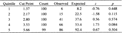
Table 6.4 presents the observed and estimated expected numbers of events, the z-score and two-tailed p-value within each quintile of risk for the fitted model in Table 6.3. The results in the observed and expected columns of Table 6.4 are obtained as follows: (1) Following the fit of the model in Table 6.3, we saved the martingale residuals and risk score; (2) We sorted the risk score and created a grouping variable with values 1 – 5 based on the quintiles of the risk score; (3) We calculated the observed number of events in each quintile by summing the censoring variable over the subjects in each quintile. For example, the sum of the follow up status (censoring) variable over the 100 subjects in the first quintile is 6; (4) We created the model cumulative hazard by subtracting the martingale residual from the follow up status (censoring) variable; and (5) We calculated the expected number of events in each quintile by summing the cumulative hazard over the subjects in each quintile. For example, the sum of the cumulative hazard over the 100 subjects in the first quintile is 8.2. We note that, unlike the goodness of fit test in logistic regression, the value of the test statistic is cannot be obtained by summing over the five rows in Table 6.4. It must be calculated using either the score or likelihood ratio test for the inclusion of four reference cell design variables formed from the quintile grouping variable. Any one of the five groups may be used as the reference value.
The numbers in Table 6.4 are large enough for all the five quintiles of risk and we feel comfortable using the normal approximation to the Poisson distribution. With a p-value equal to 0.084, only the fourth quintile has a borderline significant difference between the observed and model-based expected count. We conclude that there is sufficient agreement between observed and expected number of events within each of the five quintiles of risk. The model displayed in Table 6.3 has passed the test for a good fitting model.
As in all regression analyses, some measure analogous to R2 may be of interest as a measure of model performance. As shown in a detailed study by Schemper and Stare (1996), there is not a single, simple, useful, easy to calculate and easy to interpret measure for a proportional hazards regression model. In particular, most measures depend on the proportion of censored values. A perfectly adequate model may have what, at face value, seems a low R2 due to a high percentage of censored data. In our opinion, further work needs to be done before we can recommend one measure over another. However, if one must compute such a measure, then
![]()
Table 6.4 Observed Number of Events, Estimated Number of Events, z-Scores, and Two-Tailed p-values within Each Quintile of Risk Based on the Model in Table 6.3
is perhaps the easiest and best one to use, where Lp is the log partial likelihood for the fitted model with p covariates, and L0 is the log partial likelihood for model zero, the model with no covariates. For the fitted model in Table 6.3, the value is
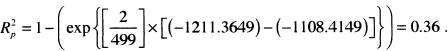
![]() has been suggested by Nagelkerke (1991). Two other measures that extend
has been suggested by Nagelkerke (1991). Two other measures that extend ![]() and are easy to calculate have been suggested by O’Quigley, Xu and Stare (2005) and Royston (2006). The measure suggested by O’Quigley et al. replaces n in
and are easy to calculate have been suggested by O’Quigley, Xu and Stare (2005) and Royston (2006). The measure suggested by O’Quigley et al. replaces n in ![]() by the number of events and is thus less dependent on the percentage of censored observations. This measure is termed “measure of explained randomness”
by the number of events and is thus less dependent on the percentage of censored observations. This measure is termed “measure of explained randomness”
![]()
where m is the number of events observed. To obtain a measure that more closely resembles the measure of explained variation for linear regression, Royston (2006) suggests using
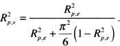
For the fitted model in Table 6.3, these two measures yield ![]() = 0.65 and
= 0.65 and ![]() = 0.53 . This illustrates that different measures of explained variation or randomness can yield quite different values for the same model.
= 0.53 . This illustrates that different measures of explained variation or randomness can yield quite different values for the same model.
We are now in a position to discuss the interpretation of this model and how best to present the results to the audience of interest.
6.6 INTERPRETING AND PRESENTING RESULTS FROM THE FINAL MODEL
The model fit to the WHAS500 data, shown in Table 6.3, is reported again in Table 6.5. It is an excellent model for teaching purposes, as it contains examples of many of the complications that we are likely to encounter in practice. The model contains a simple dichotomous covariate (chf), two continuous linear covariates (hr and diasbp), a continuous non-linear covariate (bmi) and an interaction between a continuous and a dichotomous covariate (age and gender). In this section, when we refer to “the model”, it is the one in Table 6.5.
We begin by discussing how to prepare point and interval estimates of hazard ratios for the covariates. Note that we have avoided including any exponentiated coefficients in tables of estimated coefficients in Chapters 5 and 6. While most software packages automatically provide these quantities, they are likely to be useful summary statistics for only a few model covariates. We feel it is best not to attempt estimating any hazard ratios until one has completed all steps in both model development and model checking (i.e., we want to be sure that the model fits, that it satisfies the proportional hazards assumption, and that any and all highly influential subjects have been dealt with in a scientifically appropriate manner).
Only the covariates for heart rate and diastolic blood pressure appear as linear main effects, and congestive heart problems is the only categorical covariate not involved in an interaction. As a result, these have hazard ratios that may be estimated by exponentiating their estimated coefficients. It is convenient to display these estimated hazard ratios and their confidence intervals in a table similar to Table 6.6.
The estimated hazard ratio for a 10-beat/min increase in heart rate is 1.13 = exp(l0x0.012). This means that subjects with a 10-beat/min higher heart rate are dying at a 13 percent higher rate than are subjects at the lower heart rate. The 95 percent confidence interval in Table 6.6 suggests that an increased rate of dying as high as 20 percent or as little as a 7 percent is consistent with the data.
Table 6.5 Estimated Coefficients, Standard Errors, z-Scores, Two-Tailed p-values, and 95% Confidence Interval Estimates for the Final Proportional Hazards Model for the WHAS500 data, n = 499
Because the model is linear in heart rate, this interpretation holds over the observed range of heart rate.
The estimated hazard ratio for a 10-mm/Hg increase in diastolic blood pressure is 0.89 = exp(10 ×–0.012). Thus, subjects with a 10-mm/Hg higher blood pressure are dying at a rate 11 percent lower than are subjects with lower blood pressure. The 95 percent confidence interval in Table 6.6 suggests that a decrease in the rate of dying could be as much as 17 percent or as little as 5 percent with 95 percent confidence. Because the model is linear in diastolic blood pressure, this interpretation holds over the observed range of diastolic blood pressure.
The estimated hazard ratio for congestive heart complications is 2.29 = exp(0.830). Subjects who have congestive heart complications at study entry are dying at a rate 2.29 times higher than those subjects who do not have congestive heart complications. The 95 percent confidence interval in Table 6.6 indicates that the rate could actually be as much as a 3.06-fold or as little as a 1.72-fold increase in the rate of dying.
When a study is aimed at the effect of a single treatment or risk factor of interest, the hazard ratio is often presented for only this covariate, with the other covariates in the model relegated to footnote status. We feel that this is not good statistical or scientific practice. With such an oversimplified summary, the reader has no way of evaluating whether an appropriate model building and model checking paradigm has been followed or what the actual fitted model contains. We feel that the full model should be presented in a tablesimilar to Table 6.5 at some point in the results section.
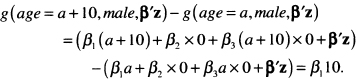
Age and gender are present in the model, with both main effects and their interaction. Because gender is dichotomous, we present hazard ratios for gender at various ages and then the hazard ratio for increasing age for each gender. The process is essentially the same for both. We first write the equation for the log hazard as a function of the variables of interest, holding all the others fixed,
![]()
Table 6.6 Estimated Hazard Ratios and 95% Confidence Interval Estimates for Heart Rate and Congestive Heart Complications for the WHAS500 Study,n =499
| Variable | Hazard Ratio | 95% CIE |
| Heart Rate | 1.13* | 1.07, 1.20 |
| Diastolic Blood Pressure | 0.89* | 0.83, 0.95 |
| Congestive Heart Complications | 2.29 | 1.72, 3.06 |
* Hazard ratio for a 10 beat/min increase.
# Hazard ratio for a 10 mm/Hg increase.
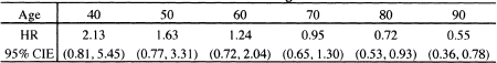
Table 6.7 Estimated Hazard Ratios and 95% Confidence Interval Estimates for the Effect of Female Gender at the Stated Values of Age
where β′z denotes the contribution to the log hazard of the other five model covariates.
We then write the expression for the difference of interest, in this case, female versus male with age fixed:
(6.27)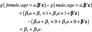
Next, choose a value for age, say 50, and estimate the hazard ratio using the exponentiated value of (6.27) with the estimated coefficient of gender from Table 6.5, ![]() 2 = 1.838 , and the estimated coefficient of the interaction of age and gender,
2 = 1.838 , and the estimated coefficient of the interaction of age and gender, ![]() 3 = –0.027 . The estimated hazard ratio at age 50 is
3 = –0.027 . The estimated hazard ratio at age 50 is
![]()
The endpoints of the 100(1 –α) percent confidence interval estimator of the hazard ratio are computed by exponentiating the endpoints of the confidence interval of the estimator of (6.27), which are
(6.28)![]()
where
(6.29)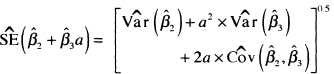
The values of the variances and covariance needed to compute the standard error are available from software packages. In this example, these are
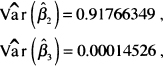
and
![]()
We present many decimal places for the variances and covariance as a reminder that rounding should be done at the final step if values are calculated manually. Using these values, the 95 percent confidence interval at age 50 is (0.77,3.31). Confidence interval estimates at the other values of age in Table 6.7 are computed in a similar manner. Because the value 1.0 is contained in the confidence interval, the estimated increase in the rate of dying is not significant. The value 1.0 is also contained in all the confidence intervals for ages 40, 60, and 70. At age 80, the model estimates that females are dying at a rate 28 percent lower than males. The estimated decrease is significant, as 1.0 is not in the confidence interval and could be much as 47 percent or as little as 7 percent, with 95 percent confidence. By age 90, females are estimated to be dying at a rate 45 percent less than males. However, only 29 of the 499 subjects are 90 or older.
The results in Table 6.7 show that, by including the significant age by gender interaction in the model, we are able to refine the estimate of the gender effect to be significant only for age 80 or older. Had we not included this interaction, we would have incorrectly concluded that females have a significantly decreased rate at all ages (e.g., fit the main effect model in Table 5.9 excluding the subject with id number 416).
The estimated gender-specific hazard ratios for a 10-year increase in age are computed following the same procedure. For males the difference in the log hazards is
For females the difference in the log hazard is
The estimated hazard ratios using the fitted model in Table 6.5 are 1.82 = exp(0.060 × l0) for males and 1.39 = exp[(0.060-0.027)× 10] for females. Because the hazard ratio for males only involves the main effect coefficient, the end points of its 95 percent confidence interval are easily obtained by multiplying the end points in Table 6.5 for the coefficient by 10 and then exponentiating, yielding the interval (1.54,2.14). The required standard error of the log hazard ratio for females is
![]()
The estimate of ![]() is shown above and other estimates are
is shown above and other estimates are ![]() = 0.00006937 and
= 0.00006937 and ![]() = –0.00006033. Using these values, the 95 percent confidence intervals are (1.54,2.14) for males and (1.14,1.67) for females.
= –0.00006033. Using these values, the 95 percent confidence intervals are (1.54,2.14) for males and (1.14,1.67) for females.
This means, that for each 10-year increase in age, the rate of dying among males increases 1. 82 fold; this increase could be as little as 1.54 fold or as much as 2.14 fold with 95 percent confidence. For females the effect of increasing age is less, 1.39 fold, but is still significant. In practice, the estimates and their confidence intervals could be included in a table similar to Table 6.6, in a separate table, or simply described in the results section. Whichever format is used, one must be sure to include the age increment in the presentation.
Body mass index is modeled with two non-linear terms, so any hazard ratio will depend on the values of body mass index being compared. The graph in Figure 5.3 of the log hazard using the two non-linear terms shows a decrease in the log hazard until the minimum is reached at about 31.5 kg/nr followed by an asymmetric increase. The most logical and informative presentation in this case would compare the hazard ratio relative to the minimum value. These hazard ratios could either be tabulated or presented graphically, along with their confidence limits. Both are illustrated here.
One must proceed carefully when calculating hazard ratios for nonlinear functions of a covariate. First, write down the expression for the log-hazard function, keeping all other covariates constant. For ease of presentation, let the log-hazard function computed at a particular value of body mass index, bmi, holding all other covariates fixed and denoted as z, be
![]()
where
![]()
and
![]()
The next step is to write down the equation for the difference of interest in the log hazard function. For any fixed value of bmi (bmi = bmic ) it is
![]()
where
![]()
and
![]()
The estimator of the hazard ratio is
(6.30)![]()
The estimator of the endpoints of the 100(1-α) percent confidence interval for the difference in the log-hazard functions is
(6.31)![]()
where
![]()
The estimators of the variances and covariance in (6.32) are obtained from output of the covariance matrix of the estimated coefficients from software packages. In the current example these values are ![]() = 0.0303041,
= 0.0303041, ![]() = 0.00156365 , and
= 0.00156365 , and ![]() = –0.0068076 . The endpoints of the confidence interval estimator for the hazard ratio are obtained by exponentiating the estimators in (6.31).
= –0.0068076 . The endpoints of the confidence interval estimator for the hazard ratio are obtained by exponentiating the estimators in (6.31).
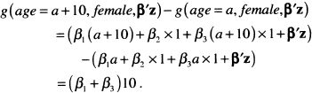
We calculated the value of the hazard ratio in (6.30) for the entire range of bmi and have graphed it, along with its 95 percent confidence bands, in Figure 6.9. One subject with bmi = 44.84 is excluded from the plot, as the upper confidence limit is 16.3, which when included, greatly distorts the appearance of the plot and hinders interpretation.
The plot in Figure 6.9 clearly demonstrates that, in the WHAS500 data, the rate of dying relative to the model-based minimum at 31.5 decreases and then in creases in an asymmetric manner. While difficult to see in Figure 6.9 a listing of the values shows that 1.0 is contained in the confidence limits for body mass index between the values of 26.9 and 39.9. Thus, there is a significant increase in the rate of dying for body mass index less than 26.9 and greater than 39.9.
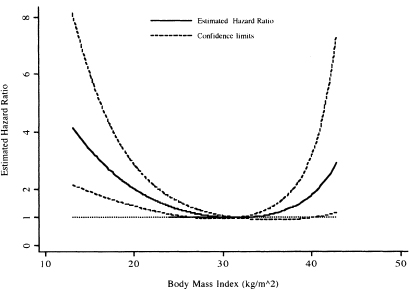
The plot in Figure 6.9 provides an easily understood description of the overall change in the estimated hazard ratios. However, it is not possible to read details at specific values of body mass index; for this we need a table. As an example, we show in Table 6.8 the estimated hazard ratios and 95 percent confidence limits for selected values of body mass index. The results in Table 6.8 show that a body mass index of 20 or less increases by more than two-fold the estimated rate of dying compared with a body mass index of 31.5. Results similar to those in Figure 6.9 and Table 6.8 can easily be obtained using a different referent value, for example 25.0, by replacing 31.5 in all expressions with the new value.
Figure 6.9 Estimated hazard ratio and 95 percent confidence bands comparing each value of body mass index to the model-based minimum-risk value of 31.5 with a referent line at 1.0 added for interpretation.
Before moving on, we want to emphasize the fact that, in this section, we have had to describe both the calculation and interpretation of the estimated hazard ratios. In practice, the estimated hazard ratios and their confidence intervals would likely be tabulated or graphed with no computational details presented and thus lend themselves to a discussion with more continuity than was possible here. However, for a complicated nonlinear variable like the body mass index, inclusion of an appendix providing an outline of how the graphed (or tabulated) hazard ratios and their confidence intervals have been computed can be a helpful addition to a paper.
We also note that we were somewhat surprised that the lowest hazard ratio was estimated to occur for a body mass index of 31.5. Individuals with a body mass index of 30 or larger are considered obese (underweight if bmi < 18.5, normal weight if 18.5 ≤ bmi < 25, overweight if 25 ≤ bmi < 30) and would typically not be at reduced risk for most health outcomes. This particular sample might be biased because body mass index was not recorded on all patients and thus a selection bias could have occurred. Nevertheless, the non-linearity in the log hazard of bmi provides a good example of how to detect and model non-linearity.
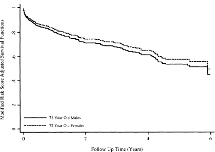
We conclude our presentation of the fitted model in Table 6.5 with graphs of the covariate-adjusted survival functions. In the WHAS500 data, no one variable can be regarded as the most important risk factor. Thus, with these data, we might choose to provide covariate adjusted survival functions at various quantiles of the risk score, as illustrated in Figure 4.7. However, for demonstration purposes we consider an example of plotting that is a bit more complicated than that of a dichotomous covariate. Suppose that we would like the covariate adjusted survival functions for 72-year-old males and 72-year-old females. Because the model is complicated and includes the gender-by-age interaction, it is not clear what we could use for a mean or median subject, so we use the modified risk score method discussed in Section 4.3 and illustrated in (4.28) and (4.29). The modified risk score is calculated for each subject as
![]()
and the median is ![]() = –1.75464. The plotted points for the covariate-adj usted survival function for 72-year-old males are
= –1.75464. The plotted points for the covariate-adj usted survival function for 72-year-old males are
Table 6.8 Estimated Hazard Ratios and 95% Confidence Interval Estimates for the Effect of Body Mass Index (BMI) Compared with Body Mass Index = 31.5
![]()
and for 72-year-old-females they are
![]()
Graphs of these two functions are shown in Figure 6.10 over the first 6 years of follow up. The survival functions in Figure 6.10 are consistent with the estimated hazard ratios in Table 6.7, which indicate a slightly reduced and not significant rate of dying at age 72. Actual calculation shows that the estimated hazard ratio at 72 years is 0.87, or a 13 percent reduction in the rate of dying. The curves are each plotted over the same subjects and are constrained to have this hazard ratio at all plotted values.
The modified risk score adjusted 75th percentiles may be estimated, albeit crudely, from the plots in Figure 6.10 or from a time-sorted list of the functions. The values are 1.92 years for 72-year-old females and 1.5 years for 72-year-old males. As noted in Section 4.5, there is no easily computed confidence interval for the estimator of the percentiles time from a modified risk-score-adjusted survival function.
Figure 6.10 Graphs of the modified risk score adjusted survival functions for 72-year-old males and 72-year-old females using the fitted model in Table 6.5.
In conclusion, the fitted model, shown in Table 6.5, has allowed description of a number of interesting relationships between time to death following an admission to the hospital after an MI and patient characteristics on admission. The notable results include significant effects due to heart rate, diastolic blood pressure, and congestive heart complications, differential effects of age within each gender, differential effect of gender for age, and the nonlinear effect of the body mass index.
In the next chapter, we consider alternative methods for modeling study co-variates. These methods are of interest in themselves, but they also provide alternatives to models that are inadequate due to poor fit or violations of the proportional hazards assumption.
1. Using WHAS100 data, assess the fit of the proportional hazards model containing age, body mass index, gender, and the age-by-gender interaction. This assessment of fit should include the following steps: evaluation of the proportional hazards assumption for each covariate, examination of diagnostic statistics, and an overall test of fit. If the model does not fit or adhere to the proportional hazards assumption what would you do next? Note: the goal is to obtain a model to estimate the effect of each covariate.
2. Using the model obtained at the conclusion of Problem 1, present a table of estimated hazard ratios, with confidence intervals. Present graphs of the modified risk score adjusted survival functions at the three quartiles (25th, 50th, and 75th) of body mass index. Use the estimated survival functions to estimate the median survival time for each of the three risk groups
3. In Section 6.4 diagnostic statistics were plotted and 10 subjects, shown in Table 6.2, were identified as being possibly influential. Fit the model shown in Table 6.5, deleting these subjects one at a time and then, collectively, calculate the percentage change in all coefficients with each deletion. Do you agree or disagree with the conclusion to delete subject 416? Explain the rationale for your decision.
4. An alternative model considered but not used in Section 5.2 is one that contains an age-by-congestive heart problem interaction in place of the age-by-gender interaction. Perform all the model evaluation and fit steps performed in problem 1 on the alternative model.
5. Repeat problem 2 using the model from problem 5.
6. Repeat problems 1 and 2 for the ACTG320 model from Problem 2 in Chapter 5. Plot modified risk score adjusted survival functions for the two levels of treatment.