
CHAPTER 7
Extensions of the Proportional Hazards Model
Up to this point, we have made several simplifying assumptions in developing and interpreting proportional hazards models. We have used a model with a common unspecified baseline hazard function where all the study covariates had values that remained fixed over the follow-up period. Additionally, we have assumed that the observations of the time variable were continuous and subject only to right censoring. In some settings, one or more of these assumptions may not be appropriate.
We may have data from a study in which subjects were randomized within study sites. If we account for site by including it as a covariate, the model forces the baseline hazards to be proportional across study sites. This may not be justified and, if it is not, a careful analysis of the proportional hazards assumption (as discussed in Chapter 6) for site may reveal the problem. One possible solution is to use site as a stratification variable, whereby each site would have a separate baseline hazard function. This same line of thought might apply to cohort year in the Worcester Heart Attack Study. Also, stratification can sometimes be employed with fixed covariates that, on testing, show evidence of non-proportional hazards.
When study subjects are observed on a regular basis during the follow-up period, the course of some covariates over time may be more predictive of survival experience than were the original baseline values. For example, continued survival of intensive care unit patients may depend more on changes in covariates that measure their physiologic condition since admission than on their values at admission. Covariates whose values change over time are commonly called time-varying or time-dependent covariates. These may include measurements on individual subjects or measurements that record study conditions and apply to a number of study subjects.
Suppose that, in the process of model checking, we determine that the hazard function is non-proportional in one or more of the covariates. We may include in the model an explicit function of the covariate and time, which is essentially the test for non-proportional hazards described in Chapter 6. In some settings, this may provide a useful solution to the problem. A similar approach is to partition the time axis and to fit different functional forms for the covariate within time intervals. We could use the smoothed plots of the scaled Schoenfeld residuals to identify the intervals where the “slope” was the same. In general, we would not attempt such an analysis unless there was strong evidence for it from subject matter considerations, statistical tests, and plots of the type discussed in Chapter 6.
While right censoring is by far the most frequently encountered censoring mechanism, there may be settings in which incomplete observations arise from other types of censoring. Thus, it may be necessary to model the data taking into account a variety of different censoring patterns.
In settings in which subjects are not under continual observation, but rather their follow-up status is determined at “fixed” intervals, another problem may arise. For example, if we are studying survival of patients admitted to a coronary intensive care unit who were discharged alive, we may contact subjects at 3-month intervals. All that may be known on the subjects is their vital status at these interval points, and the recorded values of time would be 3, 6, 12, and so on. Such data are highly discrete and, in this setting, we should consider using an extension of the proportional hazards model designed to handle interval censored data.
These and other topics that extend the basic proportional hazards model are discussed in some detail in this chapter. We begin with the stratified proportional hazards model.
7.2 THE STRATIFIED PROPORTIONAL HAZARDS MODEL
The rationale for creating a stratified proportional hazards model is the same as that for other stratified analyses. We assume there are variables known to affect the outcome, but we consider obtaining estimates of their effects to be of secondary importance to those of other covariates. These covariates might be fixed by the design of the study or they might have been identified in earlier analyses. For example, in the Worcester Heart Attack Study, patients are identified by the calendar year of their admission. In previous chapters, we ignored cohort year. The stratified proportional hazards model is also sometimes used to accommodate non-proportional hazards in a covariate.1
The stratified proportional hazards model is, in spirit, quite similar to the one used in a matched logistic regression analysis [see Hosmer and Lemeshow (2000, Chapter 7)]. The effect of all covariates whose values are constant within each stratum is incorporated into a stratum-specific baseline hazard function. The effects of other covariates may be modeled either with a constant slope across strata or with different slopes. For example, in the model developed for the WHAS500 data in Chapters 5, we assumed that covariate effects were constant over cohort years. Because cohort year is not of interest by itself, we could stratify on it and then include cohort year by covariate interactions to determine whether there is evidence of a change in effect over calendar years. In general, this modeling decision, based on the slopes being equal or unequal, may be made based on subject matter considerations or by using the methods for selecting interactions discussed in Chapter 5.
We now describe the stratified proportional hazards model using constant slopes. We note that the non-constant slopes model may be handled simply by specifying an interaction between one of the covariates and the stratification variable. The proportional hazard function for stratum as is
(7.1)![]()
where we assume there are s = 1,2,...,S strata. In the WHAS500 data, there are s =3 strata denoting the three years data were collected.
Hazard ratios are computed using the estimated coefficients and apply to each stratum. For example, in a stratified model, suppose that the estimated coefficient for a dichotomous covariate is In(2), hence the stratum-specific estimated hazard ratio is 2. The interpretation of this hazard ratio is the same as in the unstratified model, that is, the hazard rate in the x = 1 group is twice the hazard rate in the x = 0 group, and this interpretation applies to each stratum.
The form of the partial likelihood for the sth stratum is identical to the partial likelihood used in earlier chapters, see (3.19), but it includes an additional subscript, s, indicating the stratum. The contribution to the partial likelihood for the sth stratum is
(7.2)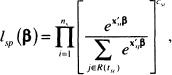
where ns denotes the number of observations in the sth stratum, tsi denotes the ith observed value of time in the sth stratum, csi is the value of the 0/1 censoring variable associated with tsi , R(tsi) denotes the subjects in stratum s in the risk set at time tsi , and Xsi is the vector of p covariates. The full stratified partial likelihood, is obtained by multiplying the contributions to the likelihood, namely
(7.3)![]()
The subscript s is used in (7.3) to differentiate the stratified partial likelihood from the unstratified partial likelihood, lp (β), used in previous chapters. The maximum stratified partial likelihood estimator of the parameter vector, β, is obtained by solving the p equations obtained by differentiating the log of (7.3) with respect to the p unknown parameters and setting the derivatives equal to zero. We do not provide these equations because they are quite similar in form to those in (3.31). The only difference is that the weighted risk set covariate means are based on the data within each stratum. The estimator of the covariance matrix of the estimated coefficients is obtained from the inverse of the observed information matrix in a manner similar to the unstratified setting, see (3.32)–(3.34).
The general steps in model building and assessment are the same for the stratified model as for the unstratified model, the only difference is that the stratified analysis is based on the partial likelihood in (7.3). The stratified analysis of the WHAS500 data using year as a stratification variable would require that we repeat all the steps in Chapters 5 and 6 relevant to model building and assessment. Repeating these steps would not demonstrate anything new. While providing a convenient conceptual example, a fit of the model in Table 6.3 stratifying on year yields estimated coefficients that differ by less than 10 percent from the estimates in Table 6.3. Hence, little would be gained by further consideration of the WHAS500 data. Instead we turn to the ACTG320 study.
Using the purposeful selection paradigm in Chapter 5, we obtain a model containing the following covariates in Table 1.5: treatment indicator (tx), IV drug history dichotomized (ivdrug_d: 0 = never, 1 = ever), two design variables for Karn-ofsky performance scale using the value of 100 as the reference and pooling the subjects in the two categories karnof = 70 and karnof = 80 as only 32 subjects have a value of 70, age, and CD4 count. There is no evidence of non-linearity in the log hazard for age and CD4 count. Also, there are no significant interactions among the model covariates. Checking the assumption of a proportional hazard for each model covariate shows that there is some evidence of a non-proportional hazard in CD4 with p-values ranging from 0.07 to 0.12 for the four tests discussed in Section 6.3. The effect of CD4 count on survival among AIDS patients is well known. In these data, we do not have continuing measures of CD4 count, only its value at baseline. Thus we create a categorical variable, based on the observed CD4 quartiles, and stratify on it. While the categorical variable is constant within strata, the measured values are not. Thus, we could include CD4 in the stratified model as well. When it is included, its estimated coefficient is not significant with a Wald test p = 0.22. The results of the fitted stratified model are shown in Table 7.1.
Table 7.1 Estimated Coefficients, Standard Errors, z-Scores, Two-Tailed p values, and 95% Confidence Intervals for the Proportional Hazards Model Stratified by CD4 Quartile for the ACTG320 data (n = 1151)
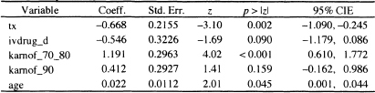
Log-likelihood = -506.7552
After a stratified model has been fit, the methods described in Section 3.5 may be used to estimate stratum-specific baseline survival functions. These functions may then be used to estimate covariate-adjusted, stratum-specific, survival functions using the methods described in Section 4.5.
In the current example, we denote the estimators of the stratum-specific baseline survival function as ![]() because CD4 was coded into quarti les. The fitted model in Table 7.1 is modestly complicated; we choose to use the modified risk score approach to obtain graphs to describe the effect of treatment within each stratum [see (4.30)-(4.31)|. Because this estimate is to be made within strata, and because the distribution of the risk score could be different across strata, we favor using stratum-specific median modified risk scores. The median values, based on the fitted model in Table 7.1, are
because CD4 was coded into quarti les. The fitted model in Table 7.1 is modestly complicated; we choose to use the modified risk score approach to obtain graphs to describe the effect of treatment within each stratum [see (4.30)-(4.31)|. Because this estimate is to be made within strata, and because the distribution of the risk score could be different across strata, we favor using stratum-specific median modified risk scores. The median values, based on the fitted model in Table 7.1, are ![]() for quartile 1,
for quartile 1, ![]() for quartile 2,
for quartile 2, ![]() for quartile 3, and
for quartile 3, and ![]() for quartile 4.
for quartile 4.
It follows that the estimators for the stratum-specific modified risk-score-adjusted survival functions for the two treatments within each stratum are described by the equations
(7.4)![]()
and
(7.5)![]()
where ![]() is the value of the median modified risk score within stratum s and -0.668 is the estimated coefficient of treatment from Table 7.1.
is the value of the median modified risk score within stratum s and -0.668 is the estimated coefficient of treatment from Table 7.1.
Figure 7.1 Graphs of the stratum-specific modified risk-score-adjusted survival functions for control (---) and treatment (—). Note the differences in scales.

In Figure 7.1 we present the graphs of the treatment by stratum-modified risk-score-adjusted survival functions. The range of the estimated survival functions is different for each stratum and the scales have been adjusted accordingly. In each of the four figures, the lower function corresponds to the modified risk-score-adjusted survival function for the control treatment while the upper curve is that of the “treatment,” which is the same as the control plus IDV (see Section 1.6). The distance between the two curves for each stratum is such that the estimated hazard ratio for treatment versus control is
![]()
with a 95 percent confidence interval estimate of (0.336,0.782). Thus the that inclusion of IDV reduces the rate of death and/or time to AIDS diagnosis by almost 50 percent; the reduction could be as little as 22 percent or as much as 66 percent with 95 percent confidence.
The modified risk-adjusted survival functions may be used in the same manner illustrated in Section 6.6 to obtain estimates of adjusted quantiles of time to death or AIDS diagnosis. Because the ranges are different within each stratum and none include even the 75th percentile, one would question the value of this application in this example.
As we have noted, the stratified proportional hazards model may be the best model to use in a setting in which covariates have values fixed by the design of the study. As we illustrate with the ACTG320 data, using a stratified analysis can provide the possibility for a simple solution to non-proportional hazards in a co-variate. In all cases, one must pay attention to the number of observations and survival times within each stratum. Small numbers within any stratum will result in an estimated baseline survival function with greater variance than the estimates from strata with more data. However, the variance of the estimates of the coefficients in a stratified model is, as before, a function of the total sample size and total number of survival times.
Until now we have assumed that the values of all covariates were determined at the point when follow-up began on each subject (time zero) and that these values did not change over the period of observation. There may be situations where one or more of the covariates are measured during the period of follow up and their values change. In these settings, it may be the case that the value of the hazard for the event depends more on the current values of these covariates than on their values at time zero.
It is not difficult to generalize the proportional hazards regression model and its partial likelihood to include time-varying covariates. However, from a conceptual point of view, the model becomes much more complicated, and one should give serious consideration to the nature of any time-vary ing covariate before including it in the model. Specifically, one must pay close attention to the definition of when the analysis time is zero (i.e., when the “clock starts”), because the start of analysis time may occur at different calendar times for different subjects. However, the value of any time-varying covariate must depend only on study time, not on calendar time. Another concern is the potential to overfit a model when using time-varying covariates. In all instances, inclusion of time-varying covariates should be based on strong clinical evidence. One of the earliest applications of the use of time-varying covariates in a biomodical setting may be found in Crowley and Hu’s (1977) analysis of the Stanford heart transplant data. In a summary paper, Andersen (1992) illustrates the use of time-varying covariates in several examples and discusses some of the problems we may encounter when including them in a model. Fisher and Lin (1999) also provide illustrations of the use of time-varying covariates and discuss related conceptual issues and potential problems and biases. Collett (2002) and Marubini and Valsecchi (1995) discuss time-varying covariates at a level comparable to this text, while Fleming and Harrington (1991), Andersen, Borgan, Gill and Keiding (1993) and Kalbfleisch and Prentice (2002) present the topic from the counting process point of view.
Time-varying (or time-dependent) covariates are usually classified as being either internal or external. An internal time-varying covariate is one whose value is subject-specific and requires that the subject be under periodic observation. For example, consider a clinical trial for a new cancer treatment in which the endpoint is death from the cancer. Suppose that we have a covariate measured at baseline, but whose value can change over time. It may be the case that the hazard depends on a more recent value than on the baseline value. For values of this covariate to be measured during the follow up period, the subjects in this study must be under direct observation. In contrast, an external time-varying covariate is one whose value at a particular time does not require subjects to be under direct observation. Typically, these covariates are study or environmental factors that apply to all subjects under observation. For example, consider a study of a new medication for relief from symptoms of hay fever in which the time variable for the outcome records the number of hours until self-perceived relief from symptoms. In this study, an example of an external covariate is the average hourly pollen count. A subject-specific external covariate is the subject’s age. If we follow subjects for a long enough period of time, their current age may have more of an effect on survival than thei"r age when the study began. However, once we know a subject’s birth date, age may be computed at any point in time, regardless of whether the subject is still under observation. Another important external time-varying covariate is time itself. We made extensive use of this time-varying covariate in Chapter 6, where it was used to test the assumption of proportional hazards in fixed covariates via the inclusion of the interactions of the form x × g(t) in the model. In the remainder of this section, we will not differentiate between internal and external time-varying covariates.
The reader might wonder why neither age nor analysis time were modeled as a time-varying covariate in previous chapters. Age and analysis time advance in parallel if linear functions of age (or analysis time) are considered. If we were to include age as a time-vary ing covariate, the estimate of its effect would not change because any effects relating to the advancement of age would be “absorbed” into the baseline hazard function.
We need to generalize the notation to include time-varying covariates in the model. Let x(t) denote the value of the covariate x measured at time t. Assume, as we have up to this point, that we have adjusted each subject’s follow-up time to begin at zero as opposed to using real or calendar time. Thus, we assume that t determines the value of x(t) even though the same t may arise from different calendar times. For example, suppose we define a time-varying covariate as the length of stay in a hospital. Subject 1 may be admitted to a hospital on May 1 and stay in the hospital for 60 days. Subject 2 may be admitted to a hospital on July 1 and also stay in the hospital for 60 days. It is important that both subjects were in the hospital for 60 days, not that they were admitted at different times. To include such a covariate in the partial likelihood |(3.19) or (3.20)| and their multivariable equivalents, we need to account for the subject as well as for the specific time. Let xi(ti) denote the value of the covariate for subject l at time ti . To allow for multiple covariates, we let xik(ti), k = 1,2,..., p denote the value of the kth covariate for subject l at time ti and denote the vector of covariates as
(7.6)![]()
The notation in (7.6) is completely general in the sense that, if a particular covariate, xk, is fixed (i.e., not time-varying) then
![]()
and this has led some authors, for example, Andersen, Borgan, Gill and Keiding (1993), to use the time-dependent notation in (7.6) exclusively. The generalization of the proportional hazards regression function (3.7) to include possibly multiple time-vary ing covariates is
(7.7)![]()
Because the hazard function in (7.7) may depend on time in ways other than through the baseline hazard function, it is no longer proportional in the same way as when only baseline covariates are used. In most settings where time-varying covariates are included, the model will also contain fixed covariates (e.g., gender). Suppose we have a model containing the subject’s blood pressure at time t, denoted x1 (t) and gender denoted x2 . The hazard function for this model is, from (7.7),
![]()
The hazard ratio for gender is
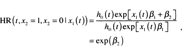
which does not depend on time. So in a sense, the hazard has a proportionality property, but the component relating to time is h0(t)exp[x1(t)β1]. This differ ence has led some authors (e.g., Collett (2003)] to drop the term “proportional” when using the model in (7.7). However, we think this might confuse the reader and, as a result, we will continue to call it the proportional hazards model because it is still proportional to a function of time, albeit one potentially much more complicated than the baseline hazard function.
A serious bias can occur when we include a time-varying covariate in the model, and the effect of a treatment on the outcome is mediated by this time-varying covariate. For example, blood pressure varies over time and could be a mediator of the effect of the treatment on outcome. In this case, inclusion of blood pressure as a time-varying covariate might bias our estimate of treatment effect because we may fail to identify a treatment effect, even if it were present. This potential problem also illustrates why modeling of time-varying covariates can be conceptually complicated.
An important assumption of the model in (7.7) is that the time-varying covariate effect, as measured by its coefficient, does not depend on time. Models with time-varying coefficients are discussed in the context of additive models in Chapter 9.
The generalization of the partial likelihood function in (3.19) is
(7.8)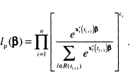
The estimators of the coefficients and their associated standard errors are obtained in a manner identical to the one described in Chapter 3, using (7.8) in place of (3.19) and (3.20). Often the biggest problem in practice is the data management necessary to describe to the software the values of the time-varying covariates. We strongly suggest that, before data collection actually begins, one consult with experts in data management for whatever software package is going to be used for model development. There is considerable variability among software packages with respect to the ease with which time-varying covariates are handled.
We illustrate modeling a time-varying covariate with two examples. The first comes from the UMARU Impact Study (UIS) described in Section 1.3 and Table 1.3. These data were used extensively in the first edition of this text. In this study, subjects were randomized to one of two residential treatment programs of different durations that were designed to prevent return to drug use. Subjects were free to leave the program at any time, and the time to event was self-reported return to drug use. We discovered that treatment appeared to have a time dependent effect. We hypothesized that the treatment effect may simply be housing a subject where he/she has no access to drugs. Here, for purposes of illustrating a time varying covariate, we begin with a univariable model containing treatment. Although we don’t present the detailed results here, the estimated hazard ratio from a fit of this model for the longer versus the shorter duration of treatment is 0.79 (95 percent confidence limits are 0.67, 0.94). Based on this model, we would conclude that longer duration of treatment significantly reduces the rate of returning to drug use. To examine the “under treatment” hypothesis, we create a time-varying dichoto-mous subject specific time varying covariate OFF_TRT(t), where
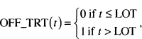
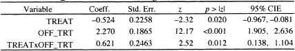
where LOT stands for the number of days the subject was on treatment. For example, consider one of the terms in (7.8) and suppose the survival time indexing the risk set is 30 days. Subjects in the risk set would have OFF_TRT(30) = 0 if their value of LOT is greater than 30, meaning that after 30 days of follow-up they were still in a treatment facility. Once the length of follow-up, t, exceeds the duration of treatment, LOT, a subject is “off treatment” and the value of OFF_TRT changes to one and remains at one as long as they are being followed. There is a considerable amount of computation involved when fitting a model with time-varying covariates. Not only must the composition of each risk set be determined, the actual values of the time-varying covariates also need to be computed. In the first edition of this text, we fit a model containing treatment and OFF_TRT(t). To provide a different example using these data, we fit a model containing TREAT, OFF_TRT (t) and their interaction. The results of this fit are shown in Table 7.2.
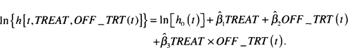
The results in Table 7.2 demonstrate a dramatic effect due to the time-varying covariate, OFF_TRT(t). We note that all three coefficients are significant. With the inclusion of the time-varying covariate and its interaction with treatment assignment, we must proceed carefully when estimating a hazard ratio. The log-hazard for the fitted model is
Table 7.2 Estimated Coefficients, Standard Errors, z-Scores, Two-Tailed p- values, and 95% Confidence Intervals for the Model Adding the Time-Varying Covariate OFF.TRT to Model Containing Treatment (n = 628)
Using this model, we can estimate four different hazards ratios: the effect of treatment assignment for subjects who are still under treatment and those off treatment and the effect of going off treatment within treatment assignment.
The log hazard ratio at time t for the effect of treatment assignment, TREAT = 1 vs, TREAT = 0, among those still on the treatment program, OFF_TRT(t) = 0, is

We obtain expressions for the other three log hazard ratios by evaluating the respective differences in the log hazards. The log hazard at time t comparing treatment assignment, long versus short, for subjects off treatment is
![]()
The log hazard at time t comparing subjects on and off treatment within the shorter treatment, TREAT = 0, is
![]()
The log hazard at time t for subjects on the longer treatment, TREAT = 1, is
![]()
The four estimated hazard ratios and their 95 percent confidence limits are shown in Table 7.3.
Table 7.3 Estimated Hazard Ratios and 95% Confidence Limit Estimates (CIE) for the Effect of Treatment and Being Off or On Treatment
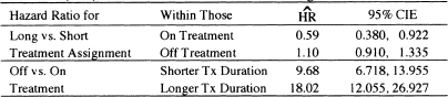
The results in Table 7.3 show that, among subjects still on treatment, those randomized to the longer of the two treatments are returning to drug use 41 percent less than subjects randomized to the shorter treatment, and this decrease is significant. Once subjects leave active treatment, there is no significant difference between the rate of returning to drug use for the longer and shorter durations of treatment. The effect of leaving treatment significantly increases the rate of returning to drug use within both levels of treatment assignment. Because the interaction effect in Table 7.2 is significant, we know that the estimated hazard ratios of 9.68 and 18.02 are significantly different.
In summary, by using a time-varying covariate that measures whether a subject has left the treatment program, we are able to obtain a much clearer picture of when the longer duration treatment is effective in reducing the rate of return to drug use as well as how the rate of return to drug use increases once subjects leave active treatment. We see clearly that this increase depends on treatment assignment. Interpretations and conclusions comparing TREAT = 1 versus TREAT = 0 do not depend on a particular value of follow up time. Instead, the value presented (i.e., the hazard ratio) is appropriate for the stated comparison (i.e., at a value of follow up time where subjects in the two programs are actively in treatment).
The stated interpretations and conclusions comparing OFF _TRT (t) = 1 versus OFF_TRT(t) = 0 require that the comparison is made for the same time t. If all patients were on treatment for exactly the same length of time and thus would go off treatment at exactly the same time, there would be no time point for which OFF_ TRT (t) = 1 for some patients and OFF_ TRT {t) = 0 for other patients. In such a case, it would not make sense to estimate and interpret the hazard ratios presented in the last two rows of Table 7.3. Nevertheless, for the UMARU Impact Study, the time points at which patients go off treatment vary greatly and the stated hazard ratios are valid for those time points where some patients are on and others are off treatment.
An alternative to the time-varying covariate analysis presented here is to fit a model with a time-dependent effect for treatment. There are four possible param-eterizations: the standard PH model with fixed covariates,
![]()
the PH model with time-varying covariates (this is the model described above using OFF_TRT(t))
![]()
the PH model where the effect depends on time but x does not change, (i.e., the setting where patients are randomized to treatment but its effect changes over time),
![]()
and the PH model where both, effect and covariate values, change over time,
![]()
We illustrate the use of the third model in Chapter 9 where we discuss a linear additive model for time to event data. We do not consider the fourth model in this book.
Data for our second example of time-varying covariates have been provided to us by Dr. Frederick Anderson, Jr, Director of the Center for Outcomes Research (COR) at the University of Massachusetts / Worcester and come from the Global Registry of Acute Coronary Events (GRACE). Data for the registry have been collected for 7.5 years from 113 Coronary Care Units (or equivalent) in 14 Countries. The registry now contains data on nearly 60,000 subjects with an acute coronary syndrome. Data from GRACE have been analyzed and reported in over 50 publications. For a paper relevant to the current example see Granger et al (2003). A complete list of GRACE publications may be found at the Center for Outcomes Research web site, www.outcomes-umassmed.org/grace.
The data we use are a blinded, specially selected sample of 1000 subjects. We thank Dr. Gordon FitzGerald of COR for his help in obtaining the sample and for discussing the use of time-varying covariates in this data set with us. A key variable for some subjects is whether they underwent a revascularization procedure such as coronary artery bypass surgery and when during their hospital i zation this procedure took place. Some subjects do not have a procedure performed; some have it performed on admission, while others have it performed some days after their admission. Of interest here is whether revascularization is associated with survival after admission. To be able to demonstrate effects, our sample of data contains proportionally more deaths (32 versus about 8 percent) and revascular-ized subjects (52 versus 38 percent) than in the full GRACE database. Hence, results presented here may not be indicative of what would be obtained if we fit the same models on the full GRACE data. The variables in our data set, called GRACE1000 are described in Table 7.4. The data set contains three baseline co-variates: age, systolic blood pressure, and an indicator of whether the baseline electrocardiogram (ECG) showed evidence of a deviation from normal in the ST segment.
Table 7.4 Description of Variables in the GRACE Data, 1000 Subjects
| Variable | Description | Values |
| id | Patient Identification Number | 1-1000 |
| days | Follow Up Time | 0.5*- 180 |
| death | Death During Follow Up | 1= Death, 0 = Censored |
| rev ase | Revascularization Performed | 1 = Yes, 0 = No |
| revascdays | Days to Revascularization After Admission | 0 – 14 if revasc = 1 and equals the value of days if revasc = 0 |
| los | Length of Hospital Stay | Days |
| age | Age at Admission | Years |
| sysbp | Systolic Blood Pressure on Admission | mm Hg |
| stehange | ST-segment deviation on index ECG | l=Yes,0 = No |
* Subjects who died or were discharged on the day they were admitted have been assigned a value of 0.5.
The naive approach to fitting a model is to treat revascularization status, revasc, as a fixed or baseline covariate. The results of fitting this model are shown in Table 7.5. Fractional polynomial analysis showed that, for these data, the log hazard is linear in the inverse of age and the square root of systolic blood pressure. Thus, in Table 7.4, we have age_inv = (1/age)× 1000 and sysbp_sqrt = ![]() . The estimated hazard ratio for revascularization is 0.59 with 95 percent confidence limits (0.468,0.741). Controlling for age, systolic blood pressure, and ST segment change, the model estimates that subjects who undergo a revascularization procedure have a rate of death during the follow up period that is 41 percent less than subjects who do not under go such a procedure.
. The estimated hazard ratio for revascularization is 0.59 with 95 percent confidence limits (0.468,0.741). Controlling for age, systolic blood pressure, and ST segment change, the model estimates that subjects who undergo a revascularization procedure have a rate of death during the follow up period that is 41 percent less than subjects who do not under go such a procedure.
Table 7.5 Estimated Coefficients, Standard Errors, z-Scores, Two-Tailed p-values, and 95% Confidence Interval Estimates for the Fitted Proportional Hazards Model Treating Revascu- larization as a Baseline Covariate (n = 1000)

The problem with the naive approach is that revascularization status is not known at admission for all subjects. For subjects who have revasc = 1 and revascdays = 0, we could argue its value is known at admission. For subjects who have revasc = 0, the fact that they did not undergo this procedure is only known at discharge from the hospital or at the time of death, if death occurs during hospitalizaron.
The correct way to model revascularization is through a time-vary ing covariate. As a first step, we treat revascularization as a dichotomous time-varying covariate similar to OFF_TRT(t) in the previous example, namely
![]()
The results of fitting this model are shown in Table 7.6. We see that the estimated coefficient for the time-varying effect of revascularization is significant with p = 0.035. The estimated hazard ratio at time t for revasc _t(t) = 1 versus revasc_t(t) = 0 is 0.77 = exp(–0.261) with 95 percent confidence limits of (0.604,0.982). The interpretation is that the rate of death among subjects who had undergone a revascularization procedure some time prior to t are dying at a rate that is 23 percent less than subjects who had not undergone a revascularization procedure prior to t, a reduction much smaller than the 41 percent from the naÏve model. It is important to note that the comparison group of subjects with revasc_t(t) = 0 includes subjects who never had the procedure, revasc = 0, as well as those who had the procedure performed after t. Because we used a dichotomous time-varying covariate, the estimate holds over all t for which comparing revasc _t(t)= 1 to revasc _t(t) = 0 is valid, i.e., t ≥l.
We see that the time varying estimate in Table 7.6 is approximately 50 percent smaller than the naÏve estimate in Table 7.5. In the naive analysis, days of follow up are incorrectly attributed to survival after revascularization from time zero to the end of follow up. For example, suppose a subject underwent revascularization on day 4 and died on day 10. In the naive analysis, all 10 days of follow up are attributed to survival after revascularization. In the correct time-varying approach, days 0 to 4 are counted toward survival without revascularization and 5 to 10 days are counted toward survival with revascularization (i.e., revasc(t) = 0 for t ≤ 4and revasc(t) = 1 for t > 4). The naïve analysis, in a sense, over-counts the days of survival due to revascularization.
Table 7.6 Estimated Coefficients, Standard Errors, z-Seores, Two-Tailed p-values, and 95% Confidence Intervals for the Fitted Proportional Hazards Model Treating Revascularization as a Time-Varying Covariate (n = 1000)
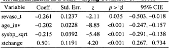
Table 7.7 Frequency Distribution of Days to Revascularization
| Days | Freq. | Percent |
| 0 | 151 | 28.9 |
| 1 | 81 | 15.5 |
| 2 | 38 | 7.3 |
| 3 | 30 | 5.8 |
| 4 | 17 | 3.3 |
| 5 | 13 | 2.5 |
| 6 | 11 | 2.1 |
| 7 | 14 | 2.7 |
| 8 | 37 | 7.1 |
| 9 | 33 | 6.3 |
| 10 | 31 | 5.9 |
| 11 | 22 | 4.2 |
| 12 | 17 | 3.3 |
| 13 | 21 | 4.0 |
| 14 | 6 | 1.2 |
| Total | 522 | 100 |
As a follow up question, suppose the clinicians on the GRACE study wanted to determine whether the effect depended on the number of days from admission to revascularization. To answer this question, we begin by examining the frequency distribution of days to revascularization (revascdays) among those who had a revascularization procedure performed. This is shown in Table 7.7. Based on these frequencies and clinical considerations, we choose to create six time-varying covariates based on having a revascularization performed on days 0, 1,2-3,4-7, 8-10, or 11-14. The time-varying covariates are defined as follows:
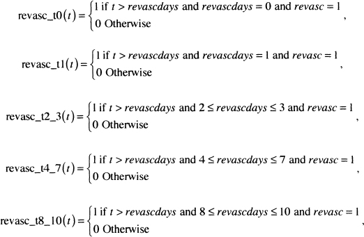
and
![]()
where t stands for days of follow up.
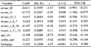
The results of fitting the model containing the six time-varying covariates are shown in Table 7.8; we see that only the time-varying covariates denoting revascularization on days 0 and 1 are significant. Using Wald tests (analyses not explicitly shown here), we find that the estimated coefficients for days 0 and 1 are not significantly different from each other, nor are the estimated coefficients for the other four time-varying covariates different from each other. The Wald tests suggest that a much more parsimonious model would be one with two time-varying covariates: One denoting days 0 and 1 and the other for days 2-14. The results of fitting the reduced model are shown in Table 7.9.
Table 7.8 Estimated Coefficients, Standard Errors, z-Scores, Two- Tailed p-values, and 95% Confidence Interval Estimates for the Fit ted Proportional Hazards Model Treating Revascularization as a Time-Varying Covariate at Six Levels (n = 1000)
Using the results in Table 7.9, we would be tempted to exponentiate the estimated coefficients for the two time-varying covariates and interpret them as estimating a hazard ratio in a manner similar to using the results in Table 7.6. However, the definition of the two time-varying covariates are linked because both cannot have a value of 1 simultaneously. Hence, we have to consider carefully which subjects have a value of zero. Suppose we let t = 5 days. At this value of time, we effectively have a categorical covariate at three levels with two design variables as described in Table 7.10. Similar coding would apply at other values of follow up time.
Based on the coding in Table 7.10 and the discussions in Section 4.2 about modeling nominal scaled covariates using reference cell coding, the reference group for the two design variables includes subjects who never had a revascularization performed and subjects who had a revascularization performed after day 4. This latter group decreases in number up to day 14, after which all revasculariza-tions had been performed. Hence, the least complicated interpretation of the estimated hazard ratios applies to days ≥ 15 when the reference group includes only those subjects who did not have a revascularization procedure preformed, revasc = 0 . These estimated hazard ratios are presented in Table 7.11.
Table 7.9 Estimated Coefficients, Standard Errors, z-Scores, Two-Tailed p-values, and 95% Confidence Interval Estimates for the Fitted Proportional Hazards Model Treating Revascularization as a Time-Varying Covariate at Two Levels (n = 1000)
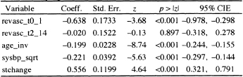
Table 7.10 Coding the Two Time-Varvinc Covariates at t = 5
| Status | revasc_t0_1(5) | revasc _t2_ 14(5) |
| { revasc = 0 } or { revasc = 1 and revascdays > 15 } | 0 | 0 |
| revasc = 1 and revasdays = 0 or | 1 | 0 |
| revasc = 1 and 2 π revascdays π 14 | 0 | 1 |
The interpretations at any time after 15 days of follow up are as follows: Subjects who had a revascularization performed on admission or one day after admission are dying at a rate that is 47 percent less than subjects who did not undergo revascularization. This difference is significant and could be as much as 62 percent less or as little as 26 percent less with 95 percent confidence. Subjects who had revascularization performed between 2 and 14 days after hospital admission are dying at a rate that is not significantly different from subjects who did not have revascularization performed. Estimates of hazard ratios at follow up times less than 15 days are the same as those in Table 7.11, but are complicated by the fact the reference group contains subjects who have not yet had a revascularization procedure, but will sometime before day 15.
In summary, by using time-varying covariates that designate revascularization status and the day on which it took place, we are able to provide correct estimates of its effect on long-term survival.
Table 7.11 Estimated Hazard Ratios and 95 Percent Con fidence Limit Estimates for the Time-Varying Effect of Revascularization at 15 or More Days of Follow Up
| Revascularization Performed On | HR | 95% CIE |
| Days 0 or 1 | 0.53 | 0.376,0.742 |
| Days 2 - 14 | 0.98 | 0.728, 1.321 |
Before leaving the example using the GRACE data, we want to remind the reader that we have used a select subset of only 1000 subjects. Thus, the results presented here do not apply to the larger GRACE database.
In each of the two examples, we used dichotomous time-vary ing covariates. We did not illustrate a setting in which the covariate varies continuously over time, as would be the case with a measured physiologic variable such as blood pressure. Inclusion of such a covariate in the partial likelihood in (7.8) is rather straightforward. The data management task of keeping track of the value(s) presents a bigger challenge. In particular, with multiple measurements, we have several choices for assigning covariate values at event times where actual values are not observed (e.g., the last measured value, the maximum of the previously measured values etc.). Hence, it is clear that, in these settings, clinical considerations of relevance to the event are vital.
Another approach to allowing the hazard function in (7.7) to change over time is to modify the baseline hazard so that it changes over time. For example, if follow up was for two years, measured in days, one might use two time-interval-specific baseline hazards defined as
![]()
It is not easy to fit such a model with coefficients that do not depend on the time interval. One way around the problem is to model the baseline hazard completely parametrically or through cubic spline functions as suggested by Royston (2001).
In Chapter 4, we discussed presentation and interpretation of covariate-adjusted survival curves. These methods were used in Section 6.6 and in the previous section. For models containing time-varying covariates, it is possible to estimate the baseline survivorship function because it does not depend on the covariates. However, it is not feasible to present individual covariate-adjusted survivorship functions; these are explicit functions of time, which is changing.
In closing, we note that time-varying covariates can provide a useful and powerful adjunct to the covariate composition of a survival time regression model. However, one should carefully consider all the implications of adding them to the model before doing so.
7.4 TRUNCATED, LEFT CENSORED, AND INTERVAL CENSORED DATA
Another simplifying assumption we have made up to this point is that the data are subject only to right censoring. That is, each observation of time begins at a well-defined and known zero value, and follow-up continues until the event of interest occurs or until observation terminates for a reason unrelated to the event of interest (e.g., the subject moves away or the study ends). In practice, this is the most frequently encountered type of survival data; however, other reasons for incomplete observation of survival time do occur. In this section, we consider some of these reasons, as well as methods for extending the proportional hazards model to address them.
Imagine the time scale for a study as a horizontal line. Incomplete observation of time can occur anywhere, but it is most common at either the beginning (i.e., on the left) or at the end (i.e., on the right) of the time scale. Censoring and truncation are the two most common causes of incomplete observation. Thus, when we consider an observation of time, we must evaluate whether the observation is subject to left censoring or left truncation and/or right censoring or right truncation. In practice, it is unlikely that an observation will be both censored and truncated on the same end of the time scale; however, an event time can be subject to incomplete observation on both sides (e.g., left truncated and right censored).
We begin with left truncation as it is, after right censoring, the next most common source of incomplete observation of survival time. To illustrate, suppose that, in the WHAS500 data, we were only interested in the survival time of patients who were discharged alive from the hospital. We define the beginning of survival time as the time the subject was admitted to the hospital. In this study, a selection process will take place in the sense that only those subjects who are discharged alive are eligible to be included in the analysis. As a result, their minimum survival time would be the length of their particular hospital stay. Observations of time that do not exceed the minimum survival time are left truncated. In this setting, all follow up times considered for the analysis must exceed some fixed value (which can be different for each individual); those subjects whose follow up times do not exceed this value are excluded from the analysis. In other words, observations subject to left truncation are not considered for the analysis.
Delayed entry is a closely related concept. Recall that the hazard rate at any time is, in the Nelson-Aalen sense, estimated by the ratio of the number of events to the number at risk. The survival experiences of subjects with delayed entry do not contribute to the analysis until time exceeds an intermediate event (being discharged alive from the hospital in the above example). Their entry into the risk sets is delayed until this intermediate event occurs. Once entered into the analysis, subjects remain at risk until they die or are right censored. The intermediate event is not reached for left-truncated values.
From a model fitting point of view, left truncation or delayed entry is difficult to handle unless the statistical software package allows counting process type data. In this data structure, each subject’s follow-up time is described by a beginning time (which need not be zero), an end time, and a right-censoring indicator variable. Currently, most of the major statistical software packages have this capability. In practice, a particular study may contain follow up times that represent all four possible combinations of left truncation and right censoring, and these are handled by the counting process style of data description. Once accounted for in the data setup, the analysis proceeds exactly as described in the previous chapters.
We use the WHAS500 data to provide an example of analysis with left truncation and delayed entry. In this sample, 461 subjects were discharged alive from the hospital. One subject is recorded as having been discharged alive but has length of follow-up equal to length of hospital stay. Thus, when delayed entry is considered, this subject does not contribute to the analysis. To illustrate the effect of delayed entry, we fit the model obtained in Chapter 5 and evaluated in Chapter 6 (see Table 6.3). The results of fitting this model are presented in Table 7.13 using delayed entry as length of hospital stay. The results in the two tables are not identical, but the interpretations and conclusions we would reach are the same.
It is not our intention to reanalyze the WHAS500 data, but rather to illustrate how to use the proportional hazards model with left-truncated or delayed entry data that is also subject to right censoring. Once delayed entry is accounted for, there are no substantive changes in the methods used for model development, assessment, and interpretation.
In summary, the key elements defining a survival time with delayed entry are: (1) the observation must, by design of the study, exceed some minimum value, that may be the same or different for all subjects, and (2) the beginning or zero value of time must be known for each observation. Andersen, Borgan, Gill and Keiding (1993) present, in Chapter III, the mathematical details as well as insightful examples involving left truncation of survival time.
Table 7.13 Estimated Coefficients, Standard Errors, z-Scores, Two-Tailed p-Values, and 95% Confidence Interval Estimates for the Final Proportional Hazards Model for the WHAS500 Data with Delayed Entry of Subjects, n = 459.

Left censoring of survival time is different from left truncation in that it occurs randomly at the individual subject level, while left truncation involves a selection process that applies to all subjects. A follow up time is left censored if we know that the event of interest took place at an unknown time prior to when the individual is first observed. Examples of left-censored data often involve age as the time variable and a life-course event. For example, in a study modeling the age at which “regular” smoking starts, the data may come from interviews of 12-year olds. A 12-year-old subject may report that he is a regular smoker but that he does not remember when he started smoking regularly. In this case, we know the observed time, 12, is larger than the time to event (i.e., the age when the subject became a regular smoker).
The defining characteristic of left-censored data is that the event is known to have occurred and the observed time is larger than the survival time. In a sense, left censoring is the opposite of right censoring, where we know that the event of interest has not occurred and that the observed time is less than the survival time.
Ware and DeMets (1976) proposed one solution for the analysis of left-censored data. They suggested turning the time scale around and treating the data as if they were right censored. This method works if the data are only subject to left censoring. In practice, however, if left censoring can occur, then right censoring is also likely to occur. In the example of age at first regular smoking, many study subjects will not be regular smokers at the time they are interviewed, and these observations of time are right censored. Alioum and Commenges (1996) present a method for fitting the proportional hazards model to arbitrarily censored and truncated data. We will not discuss their method because it is quite complex and requires computational skills greater than those assumed in the rest of this text. Klein and Moeschberger (2003) discuss general mechanisms for incomplete observation of survival time and necessary modifications in estimation methods. A somewhat simpler but less flexible approach is presented later in this section within the context of interval-censored data.
Right truncation occurs when, by study design, there is a selection process such that data are available only on subjects who have experienced the event. This typically occurs in settings where data come from a registry containing information on confirmed cases of a disease. For example, all subjects in a cancer registry, by definition, have cancer. Thus, any analysis of a time variable that uses confirmed diagnosis of cancer as the event of interest will involve right truncation. Extensions of the methods for left-truncated data or right-censored data for the analysis of right-truncated data are not especially straightforward. We will not consider analysis of right-truncated data further in this text. Instead we refer the reader to Klein and Moeschberger (2003) for a general discussion of likelihood construction and to Alioum and Commenges (1996) for methods using the proportional hazards model.
Another type of incomplete observation of time can occur if we do not know the zero value when we begin observing a subject. The observation may also be subject to right censoring. For example, in a study of survival time of patients with AIDS, suppose some subjects enter the study with active, confirmed disease, but no precise information can be obtained as to when they converted from HIV+ to AIDS. Thus, for these patients, the zero value of time, (when they actually developed AIDS) is unknown. Statistical methods have been developed to handle this setting (see DeGruttola and Lagakos (1989), Kim, DeGruttola and Lagakos (1993), Jewell (1994) and Klein and Moeschberger (2003) who describe this type of data as being doubly censored).
Interval-censored data is another form of incomplete observation of survival time that can involve left and right censoring as well as truncation. Interval censoring is used to describe a situation where a subject’s survival time is known only to lie between two values. Data of this type typically arise in studies where follow up is done at fixed intervals. For example, in the WHAS, the aim is to model the survival time among patients admitted to a hospital for a myocardial infarction. Suppose that patients who were discharged alive from the hospital were contacted every 3 months to ascertain their vital status. Patients who die before the first contact at 3 months have survival times that are left censored at 3 months. We know the event took place prior to 3 months, yet we are unsure of the exact time. All that is known is that these survival times are at most 3 months. For subjects who die between two contacts, all that is known is that survival time is at least as long as the time of the earlier contact and is no longer than the time of the most recent contact (e.g., between 9 and 12 months). For subjects still alive at their last follow up, all we know is that their survival time is at least as long as the time associated with their last contact (e.g., alive at 18 months and then lost to follow up). These observations are right censored.
Lindsey and Ryan (1998), Carstensen (1996), and Farrington (1996) have considered regression models for arbitrarily interval-censored survival time that extend methods developed by Finkelstein (1986) specifically for the proportional hazards model as well as earlier developmental work by Prentice and Gloecker (1978). Carstensen and Farrington show how arbitrarily interval-censored data may be fit by considering the problem as a binary outcome regression problem. We illustrate this approach by modifying follow-up time in the GBCS data. Collett (2003) and Klein and Moeschberger (2003) present methods for interval-censored data similar to those presented here. Sun (2006) provides a more detailed and technical discussion of interval-censored failure time data.
Assume that all we know about the observed time for the ith subject is that it is bounded between two known values, denoted ai <T ≤ bi . In addition, we know whether the event of interest occurred. The outcome is indicated by the usual censoring variable, ci = 1 if the event occurred and ci = 0 otherwise. Observations that are left censored have ai = 0 and ci = 1. Observations that are right censored have bi = ∞ and ci = 0.
Let the survival function at time t for a subject with covariate vector x, and associated parameter vector β be denoted S(t,xi,β). The probability of the observed interval for the ith subject is
(7.9)![]()
The expression in (7.9) yields [1–S(bi ,xi,β) for left-censored observations, S(ai,xi,β)–S(bi,xi,β)] for non-censored observations, and S(ai,xi,β) for right-censored observations.
The first steps in obtaining estimators of parameters in a regression model are to construct the likelihood function and then to evaluate it with the chosen model. We will use the proportional hazards model, but the method is general enough that other models could be used, including the parametric models discussed in Chapter 8. The likelihood is the product of the terms obtained by evaluating (7.9) for each subject, namely
(7.10)![]()
The computations and model fitting procedure are simplified if only a few values are possible for a and b. In this case, it is easier to refer to the interval-censored values by intervals on the time scale common to all subjects. Assume that we have J + 1 such intervals denoted (tj-1,tj] for j = 1,2,...,J + 1 with t0 = 0 and tJ+1 = ∞, and these intervals are the same for all subjects.
For ease of presentation, we let Ij denote theyth time interval (tj-1,tj]. The binary variable indicating the specific time interval observed for the jth subject is defined as
![]()
In addition, we re-express the probability for the jth interval as
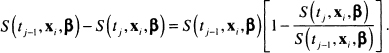
The right-most term in the square brackets in (7.11) is the conditional probability that the event occurs in theyth interval, given that the subject was alive at the end of interval ![]() . Under the proportional hazards model, the ratio of the survival function at successive interval endpoints can be simplified (algebraic steps not shown) to:
. Under the proportional hazards model, the ratio of the survival function at successive interval endpoints can be simplified (algebraic steps not shown) to:
(7.12)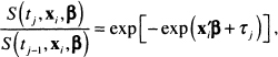
where

To further simplify the notation, let us denote the conditional probability in (7.11) as
(7.13)![]()
Using the result in (7.13), it follows that the likelihood function in (7.10) may be expressed as follows:
(7.14)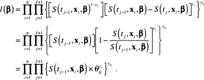
The next step involves expressing the survival function at an interval endpoint as a product of successive conditional survival probabilities, a process similar to the one used to develop the Kaplan-Meier estimator in Chapter 2, but using the expression in (7.13). The algebraic details are not shown, but the result is
(7![]()
Substituting the expression in (7.15) into the function in (7.14) results in the following likelihood function:
(7.16)![]()
Let the observed interval for the ith subject be denotedki that is, Ik, =(ai,bi,]. The first thing to note in (7.16) is that the only time the terms in the product over y differ from 1 is when j = ki . Thus the expression (7.16) simplifies to
(7.17)![]()
The likelihood function in (7.17) can be made to look like the likelihood function for a binary regression model. We define a pseudo binary outcome variable as zij = yij × ci and use it to re-express (7.17) as
(7.18)![]()
For each subject, i, (7.18) is the likelihood for ki -1+c, independent binary observations with probabilities θij and outcomes zij . This observation allows us to use standard statistical software to fit the interval-censored proportional hazards regression model.
Suppose that, in the GBCS, time to recurrence or censoring was not observed exactly, but instead only to within 12 month intervals. That is, the status of subjects was determined annually. To obtain data of this type, we form intervals by grouping follow up time in months (12 × days /365.25) into seven intervals. The first six are of length 12 months and the last interval is for follow-up time exceeding 72 months:
![]()
The results of cross tabulating the follow up times into seven intervals by the censoring indicator is shown in Table 7.13.
The first step in the model-fitting process is to expand the data for each subject ki; –1 + Ci times and create the values of y and zij . For example, in the GBCS, if a subject’s recurrence time was in the third interval, between 24 and 36 months, then ki = 3 and c, = 1. This subject would contribute 3 lines to the expanded data file. The covariates would be the same in each line; the interval indicator, y, would take on the values 1, 2, and 3; and the binary outcome variable, z, would be zero for the first 2 lines and 1 for the third line of data. If the follow up on the subject ended during the fifth interval, between 48 and 60 months without recurrence, then ki = 5 and ci = 0. This subject would contribute 5 lines of data, and the value of the binary outcome variable would be zero in all 5 lines. Similarly, if a subject’s follow-up time exceeded 72 months without cancer recurrence, then ki = 7 and ci = 0. The subject would be represented with 7 lines of data, and the binary outcome variable would be zero for each line.
Table 7.13 Frequency Distribution of the Created Interval Censored Data in the GBCS by Censoring Status (n = 686)

The binary regression model defined in (7.13) has as its link function, or linearizing transformation, the complementary log-log function, that is, lnl![]() . The design variable, represented by τj . in the model, is a 0/1 indicator variable for each time interval. All J of these variables are included in the model, which requires that we force the usual constant term to be zero.
. The design variable, represented by τj . in the model, is a 0/1 indicator variable for each time interval. All J of these variables are included in the model, which requires that we force the usual constant term to be zero.
An important point to keep firmly in mind is that the manipulations of the likelihood in (7.10)–(7.18) are designed to cast the interval-censored data problem in a form that would allow likelihood analysis by existing software. The problem is not a binary regression problem in the usual sense of the primary outcome variable being a 0/1 variable; however, we manipulated the problem to make it look like one.
The likelihood in (7.18) is identical to one that would be obtained using the general methods in Carstensen (1996) and Farrington (1996) under the restriction of a few intervals common to all subjects. If this assumption does not hold, then the more general method must be used. This method also yields a likelihood that may be analyzed using a binary regression model, but it requires a two-step fitting procedure. In addition, a second set of calculations is required to obtain standard errors of estimated model coefficients. For these reasons, we have chosen not to present the general regression method.
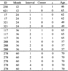
The creation of the expanded data set is more easily demonstrated using a few example subjects, shown in Table 7.14. The first line of data in this table is for a 46-year old subject who was followed for between 0 and 12 months and whose cancer had recurred some time during this interval. The second line of data is for a 65-year old subject who was followed for between 0 and 12 months and whose cancer had not recurred during this interval. These data are indicted by month = 12, interval = 1, censor = 1 or 0, and the binary outcome variable z = 1 or 0. The covariate chosen, for demonstration purposes only, is AGE.
The second block of four lines represents two subjects whose follow up time fell in the second interval. This is noted by month = 24. Subject 17’s cancer recurred in this interval, while subject 321’s did not recur. The first and third lines correspond to the fact that neither subject had a recurrence in the first year of follow up. For these lines the interval = 1 and z = 0. The second and fourth lines are for the second year of follow up, denoted by interval = 2. The recurrence for subject 17 is denoted by z = 1. The value of age is the same in both lines. Non-recurrence of the cancer for subject 321 is indicated by z = 0.
The third block of six lines represents two subjects (117 and 288): one whose cancer recurred in the third year of follow-up and one whose cancer did not recur. Both of these subjects contribute three lines of data, one for each of the three intervals. During the first two intervals of follow up, neither subject’s cancer had recurred so, for each subject, z = 0. The value is changed to z = 1 in the third line for the subject whose cancer recurred and is kept at z = 0 for the one whose cancer did not recur while being followed.
The fourth block of five lines represents a subject (278) whose cancer recurred during the fifth year of follow up. Because the subject’s cancer had not recurred during the first four intervals, z = 0 for these four lines and z = 1 for the fifth line. As in the previous examples, age remains constant at 70 in all five lines.
Data for subjects with their follow up time falling in other intervals would be expanded in a similar manner.
The technical details of expanding the data set will vary by software package, but most can perform the expansion without too much trouble. Analyses presented here were performed in STA TA, where the data expansion is especially easy to perform.
To illustrate the model fitting, we fit a model containing age, hormone use, and tumor size. Table 7.15 presents the results of fitting the interval-censored proportional hazards model containing age, hormone use, and tumor size using the likelihood in (7.18) with the expanded data set. Even though age it is not significant, we have kept it in the model because it was useful in illustrating the expanded data and is clinically important.
Table 7.14 Examples of the Expanded Data Set Re quired to Fit the Binary Regression Model in Equation (7.18) for the GBCS
The presentation and interpretation of the estimated coefficients for study co-variates in Table 7.15 would proceed in exactly the same manner as illustrated in Chapter 6 for a fitted, non-interval-censored, proportional hazards model. In this regard, it is important to remember that, even though a binary regression program was used to obtain coefficient estimates, the model generating the likelihood is the proportional hazards model.
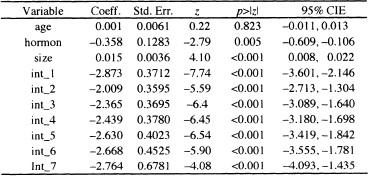
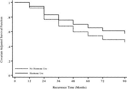
Table 7.15 Estimated Coefficients, Standard Errors, z-Scores, Two- Tailed p-values, and 95% Confidence Intervals Estimates Based on the Interval Censored Proportional Hazards Model for the GBCS Data (p = 686)
We can use the results of the fitted model and (7.15) to obtain estimates of the covariate-adjusted survival function. Because there are only seven time intervals, the survival function is not likely to be of great practical value. However, it might be of value in other settings with more intervals, so we present and illustrate the method. As in the non-interval censored setting, we begin by obtaining an estimator of the baseline survival function. In this case, the values are obtained at end-points of each interval, using the interval-specific parameter estimates. It follows from the definition of τj , and the fact that S0 (t0 = O) = 1 that the estimator of the baseline survival function at the end of the first interval is
![]()
The estimator of the baseline survival function at the end of the second interval is
![]()
In general, the estimator at the end of the jth interval, tj, is
(7.19) ![]()
for j = 1,2,...,J . As in the continuous time setting, the actual values of these estimators will not be particularly useful unless the data have been centered in such a way that having covariates equal to zero corresponds to a clinically plausible subject. We obtain the covariate-adjusted estimator of the survival function from the estimator of the baseline survival function in the same way as in the non interval-censored case, namely
(7.20) ![]()
The covariate-adjusted survival function can also be used to provide a graphical, but model-based, comparison of survival experience in groups, such as those defined by hormone use. Because the model is not complicated, we do not need to use the modified risk score approach but, instead, compare the survival curves for the two hormone use groups at the median value of age, 53 years, and tumor size, 25 mm. In doing so, we must not perform the calculations in the expanded data set because it has more than one observation or data line per subject for those whose follow up goes beyond the first interval. We must either delete the extra lines from the expanded data set or return to the original data set to perform the calculations.
The first step is to calculate the two values of the risk score. This calculation uses the coefficients for age, hormone use, and tumor size from the model in Table 7.15. The covariate adjusted risk score for no hormone use is
![]()
and the risk score for the hormone use group is
![]()
The estimated survival function for no hormone use is obtained by evaluating
![]()
for j = 0,1,...,7 . The estimated survival function for hormone use is obtained by evaluating
![]()
for y = 0,l,...,7.
Figure 7.2 presents the graphs of the two estimated survival functions. The plotted points are connected by steps to emphasize that, in the interval-censored data setting, we have no information about the baseline survival function between interval endpoints and one must assume it is constant.
The graph itself is not particularly interesting in this example because only seven intervals were used. However, in an analysis with more intervals, it could be used to provide estimates of quanti les of survival time using the methods discussed in Chapter 4 and illustrated in Chapter 6.
In summary, the modeling paradigm for interval-censored survival data is essentially the same as for non-interval-censored data. Interpretation and presentation of the results of a fitted proportional hazards model is identical for the two types of data. However, model building with interval-censored data uses the binary regression likelihood in (7.18) if intervals are the same for all subjects. This implies that model building details, such as variable selection, identification of the scale of continuous covariates, and inclusion of interactions, use techniques based on binary regression modeling. These are discussed in detail for the logistic regression model in Hosmer and Lemeshow (2001) and may be used without modification for the complimentary log-log model. However, the methods for assess ing model adequacy and fit discussed in Hosmer and Lemeshow (2001) are for use with the logistic regression model only. McCullagh and Nelder (1989, Chapter 12) discuss these methods for generalized linear models. We have not described details of how to obtain measures of leverage, residual, and influence, as well as overall goodness-of-fit from existing software packages for the complementary log-log link function.
Figure 7.2 Graphs of the covariate adjusted risk-score-adjusted survival functions for the two hormone use groups based on the fitted model in Table 7.15 for the GBCS Data (n = 686).
It is possible that survival time could be thought of as being a discrete random variable. Kalbfleisch and Prentice (2002) discuss the discrete-time proportional hazards model and show that it may be obtained as a grouped-time version of the continuous-time proportional hazards model. The grouped-time model discussed by Kalbfleisch and Prentice is identical to the interval-censored model presented in this section, so analysis of a discrete-time proportional hazards model would use the methods described in this section.
1. The model building example in Chapter 5 involved finding the best model in the WHAS500 data for lenfol (in years) as survival time and fstat as the censoring variable. The fit and adherence to model assumptions was assessed in Problem 5 in Chapter 6. In this problem and section, we call this model the “WHAS500 model.”
(a) Treating cohort year (variable: year) as a stratification variable, fit the WHAS500 model. Compare the estimated coefficients with those from the fit of the WHAS500 in Table 6.5. Are there any important differences (i.e., changes greater than 15 percent)?
(b) Are there any significant interactions between the two-design variables for cohort year (use 1997 as the reference value) and the main effects in the WHAS500 model? In these models only interaction terms are included - not the main effects for the two design variables for cohort year. If there are any significant interactions, what are they and do they make clinical sense such that they should be kept in the model?
2. An alternative approach to the analysis of long-term survival in the WHAS500 data is to study the survival experience of patients post-hospital discharge using lenfol as survival time. Restrict the analysis to patients discharged alive (dstat = 0), but account for differing lengths of stay by defining los as the delayed entry time. Note that subjects with los = lenfol should be excluded, as 0 is not an allowable value for survival time in most software packages. Examine the effect on the WHAS500 model (see Table 6.5) of this alternative method of assessing long-term survival in the WHAS. Do any of the estimated coefficients change by more than 15 percent?
3. In the GBCS data, does hormone use improve survival after cancer recurrence, controlling for tumor grade and size?
4. Does revascularization improve survival experience when the analysis of the GRACE1000 data is restricted to the 695 patients who survived hospital i zation (i.e., those patients with los π days)?
5. The survival time variable in the WHAS500 data, lenfol, is calculated as the days between the hospital admission date, admitdate, and the date of the last follow up, fdate. Follow up of patients is not done continuously but at various intervals. Thus, it is possible that a reported number of days of follow up could be inaccurate. To explore this, create a new variable monthfol = (12*lenfol/365.25). Use mnthfol to create discrete times, in multiples of 24 months (i.e., two-year intervals). For purposes of this problem, restrict analysis to the 496 subjects with, at most, 72 months of follow up.
(a) Use the method for fitting interval-censored data presented in Section 7.4, fit the WHAS500 model in Table 6.5. Compare the results of the two fitted models. Is this comparison helpful in evaluating the described grouping strategy as a method for dealing with imprecisely measured survival times?
(b) Use the fitted model in problem 3(a) and present covariate-adjusted survivorship functions comparing the survival experience of patients with and without congestive heart complications (chf).
(c) Describe a strategy for including cohort year (variable: year) as a stratification variable in the interval censored data analysis in problem 4(b). If possible, implement this strategy.
6. Data from the French Three Cities Study has been graciously provided to us by the 3C study investigators at Inserm Unit 708 in Paris, France. Data are available on approximately 8,500 subjects [see The 3C Study Group (2003)). For the purposes of this problem we eliminated subjects with missing data and sampled censored subjects yielding a data set with 697 subjects and an event rate of 10 percent. Hence results from analyses in this problem do not apply to the main study. The data are available on the web sites as FRTCS.dat and are described in FRTCS.txt.
In this study the subject’s age gender, systolic blood pressure, diastolic blood pressure and use of antihypertensive drugs are recorded at baseline. At two follow up visits the date of the visit and the measurements of systolic blood pressure, diastolic blood pressure and use of antihypertensive drugs are recorded. Hence these three covariates are examples of measured time varying covariates. The date of the event or end of follow up is recorded
(a) The first step in the analyses requires that the data for each subject be expanded from a single record to three records per subject, using the dates to create an entry time, exit time and covariate values for follow up from baseline to first follow up visit, from first follow up visit to second follow up visit and from second follow up visit to event or censoring. The single record data for the first subject are shown below: {id, age, sex (1= male, 2 = female), age, date of baseline (ddmmmyy), systolic blood pressure (mmHg) at baseline, diastolic blood pressure (mmHg) at baseline, use of antihypertensive drugs (0 = no, 1 = yes) at baseline, similar data at follow up exams one and two, date of event or end of follow up and censor (1 = event, 0 = censor)}.
![]()
The expanded data for subject 1 are shown below. The time intervals (enter and exit) are defined as the number of days from baseline. For example, 1558 is the number of days from the baseline date of 25feb99 to the second exam date of 02Jul03. Because this subject did not experience an event, censor is equal to zero at the end of all three intervals. Subjects who have an event have a value of 1 at the end of the last interval.

(b) Following the creation of the expanded data set fit a proportional hazards model, using the counting process description of follow up, containing age, sex, systolic blood pressure, diastolic blood pressure and use of antihyperten-sive drugs.
(c) Estimate and interpret hazard ratios for each model covariate.
1 Note that, if the hazard function for a continuous covariate has been identified as being nonproportional using the methods in Chapter 6, one could create a grouped or categorized version of the covariate, treat it as if it were a nominal scale covariate, and stratify on it.