Chapter 5

Procurement

We explore procurement processes in this chapter. This subject area has obvious cross-industry appeal because it is applicable to any organization that acquires products or services for either use or resale.

In addition to developing several purchasing models, this chapter provides in-depth coverage of the techniques for handling dimension table attribute value changes. Although descriptive attributes in dimension tables are relatively static, they are subject to change over time. Product lines are restructured, causing product hierarchies to change. Customers move, causing their geographic information to change. We'll describe several approaches to deal with these inevitable dimension table changes. Followers of the Kimball methods will recognize the type 1, 2, and 3 techniques. Continuing in this tradition, we've expanded the slowly changing dimension technique line-up with types 0, 4, 5, 6, and 7.

Chapter 5 discusses the following concepts:

• Bus matrix snippet for procurement processes
• Blended versus separate transaction schemas
• Slowly changing dimension technique types 0 through 7, covering both basic and advanced hybrid scenarios

Procurement Case Study

Thus far we have studied downstream sales and inventory processes in the retailer's value chain. We explained the importance of mapping out the enterprise data warehouse bus architecture where conformed dimensions are used across process-centric fact tables. In this chapter we'll extend these concepts as we work our way further up the value chain to the procurement processes.

For many companies, procurement is a critical business activity. Effective procurement of products at the right price for resale is obviously important to retailers and distributors. Procurement also has strong bottom line implications for any organization that buys products as raw materials for manufacturing. Significant cost savings opportunities are associated with reducing the number of suppliers and negotiating agreements with preferred suppliers.

Demand planning drives efficient materials management. After demand is forecasted, procurement's goal is to source the appropriate materials or products in the most economical manner. Procurement involves a wide range of activities from negotiating contracts to issuing purchase requisitions and purchase orders (POs) to tracking receipts and authorizing payments. The following list gives you a better sense of a procurement organization's common analytic requirements:

• Which materials or products are most frequently purchased? How many vendors supply these products? At what prices? Looking at demand across the enterprise (rather than at a single physical location), are there opportunities to negotiate favorable pricing by consolidating suppliers, single sourcing, or making guaranteed buys?
• Are your employees purchasing from the preferred vendors or skirting the negotiated vendor agreements with maverick spending?
• Are you receiving the negotiated pricing from your vendors or is there vendor contract purchase price variance?
• How are your vendors performing? What is the vendor's fill rate? On-time delivery performance? Late deliveries outstanding? Percent back ordered? Rejection rate based on receipt inspection?

Procurement Transactions and Bus Matrix

As you begin working through the four-step dimensional design process, you determine that procurement is the business process to be modeled. In studying the process, you observe a flurry of procurement transactions, such as purchase requisitions, purchase orders, shipping notifications, receipts, and payments. Similar to the approach taken in Chapter 4: Inventory, you could initially design a fact table with the grain of one row per procurement transaction with transaction date, product, vendor, contract terms, and procurement transaction type as key dimensions. The procurement transaction quantity and dollar amount are the facts. The resulting design is shown in Figure 5.1.

Figure 5.1 Procurement fact table with multiple transaction types.

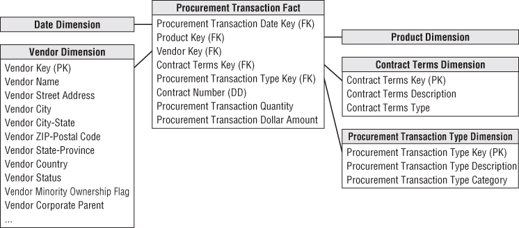
If you work for the same grocery retailer from the earlier case studies, the transaction date and product dimensions are the same conformed dimensions developed originally in Chapter 3: Retail Sales. If you work with manufacturing procurement, the raw materials products likely are located in a separate raw materials dimension table rather than included in the product dimension for salable products. The vendor, contract terms, and procurement transaction type dimensions are new to this schema. The vendor dimension contains one row for each vendor, along with interesting descriptive attributes to support a variety of vendor analyses. The contract terms dimension contains one row for each generalized set of negotiated terms, similar to the promotion dimension in Chapter 3. The procurement transaction type dimension enables grouping or filtering on transaction types, such as purchase orders. The contract number is a degenerate dimension; it could be used to determine the volume of business conducted under each negotiated contract.

Single Versus Multiple Transaction Fact Tables

As you review the initial procurement schema design with business users, you learn several new details. First, the business users describe the various procurement transactions differently. To the business, purchase orders, shipping notices, warehouse receipts, and vendor payments are all viewed as separate and unique processes.

Several of the procurement transactions come from different source systems. There is a purchasing system that provides purchase requisitions and purchase orders, a warehousing system that provides shipping notices and warehouse receipts, and an accounts payable system that deals with vendor payments.

You further discover that several transaction types have different dimensionality. For example, discounts taken are applicable to vendor payments but not to the other transaction types. Similarly, the name of the employee who received the goods at the warehouse applies to receipts but doesn't make sense elsewhere.

There are also a variety of interesting control numbers, such as purchase order and payment check numbers, created at various steps in the procurement pipeline. These control numbers are perfect candidates for degenerate dimensions. For certain transaction types, more than one control number may apply.

As you sort through these new details, you are faced with a design decision. Should you build a blended transaction fact table with a transaction type dimension to view all procurement transactions together, or do you build separate fact tables for each transaction type? This is a common design quandary that surfaces in many transactional situations, not just procurement.

As dimensional modelers, you need to make design decisions based on a thorough understanding of the business requirements weighed against the realities of the underlying source data. There is no simple formula to make the definite determination of whether to use a single fact table or multiple fact tables. A single fact table may be the most appropriate solution in some situations, whereas multiple fact tables are most appropriate in others. When faced with this design decision, the following considerations help sort out the options:

• What are the users' analytic requirements? The goal is to reduce complexity by presenting the data in the most effective form for business users. How will the business users most commonly analyze this data? Which approach most naturally aligns with their business-centric perspective?
• Are there really multiple unique business processes? In the procurement example, it seems buying products (purchase orders) is distinctly different from receiving products (receipts). The existence of separate control numbers for each step in the process is a clue that you are dealing with separate processes. Given this situation, you would lean toward separate fact tables. By contrast, in Chapter 4's inventory example, the varied inventory transactions were part of a single inventory process resulting in a single fact table design.
• Are multiple source systems capturing metrics with unique granularities? There are three separate source systems in this case study: purchasing, warehousing, and accounts payable. This would suggest separate fact tables.
• What is the dimensionality of the facts? In this procurement example, several dimensions are applicable to some transaction types but not to others. This would again lead you to separate fact tables.

A simple way to consider these trade-offs is to draft a bus matrix. As illustrated in Figure 5.2, you can include two additional columns identifying the atomic granularity and metrics for each row. These matrix embellishments cause it to more closely resemble the detailed implementation bus matrix, which we'll more thoroughly discuss in Chapter 16: Insurance.

Figure 5.2 Sample bus matrix rows for procurement processes.

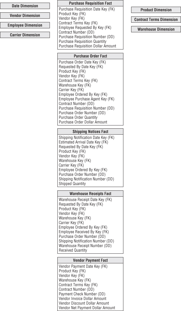
Based on the bus matrix for this hypothetical case study, multiple transaction fact tables would be implemented, as illustrated in Figure 5.3. In this example, there are separate fact tables for purchase requisitions, purchase orders, shipping notices, warehouse receipts, and vendor payments. This decision was reached because users view these activities as separate and distinct business processes, the data comes from different source systems, and there is unique dimensionality for the various transaction types. Multiple fact tables enable richer, more descriptive dimensions and attributes. The single fact table approach would have required generalized labeling for some dimensions. For example, purchase order date and receipt date would likely have been generalized to simply transaction date. Likewise, purchasing agent and receiving clerk would become employee. This generalization reduces the legibility of the resulting dimensional model. Also, with separate fact tables as you progress from purchase requisitions to payments, the fact tables inherit dimensions from the previous steps.

Figure 5.3 Multiple fact tables for procurement processes.

Multiple fact tables may require more time to manage and administer because there are more tables to load, index, and aggregate. Some would argue this approach increases the complexity of the ETL processes. Actually, it may simplify the ETL activities. Loading the operational data from separate source systems into separate fact tables likely requires less complex ETL processing than attempting to integrate data from the multiple sources into a single fact table.

Complementary Procurement Snapshot

Apart from the decision regarding multiple procurement transaction fact tables, you may also need to develop a snapshot fact table to fully address the business's needs. As suggested in Chapter 4, an accumulating snapshot such as Figure 5.4 that crosses processes would be extremely useful if the business is interested in monitoring product movement as it proceeds through the procurement pipeline (including the duration of each stage). Remember that an accumulating snapshot is meant to model processes with well-defined milestones. If the process is a continuous flow that never really ends, it is not a good candidate for an accumulating snapshot.

Figure 5.4 Procurement pipeline accumulating snapshot schema.

Slowly Changing Dimension Basics

To this point, we have pretended dimensions are independent of time. Unfortunately, this is not the case in the real world. Although dimension table attributes are relatively static, they aren't fixed forever; attribute values change, albeit rather slowly, over time. Dimensional designers must proactively work with the business's data governance representatives to determine the appropriate change-handling strategy. You shouldn't simply jump to the conclusion that the business doesn't care about dimension changes just because they weren't mentioned during the requirements gathering. Although IT may assume accurate change tracking is unnecessary, business users may assume the DW/BI system will allow them to see the impact of every attribute value change. It is obviously better to get on the same page sooner rather than later.

When change tracking is needed, it might be tempting to put every changing attribute into the fact table on the assumption that dimension tables are static. This is unacceptable and unrealistic. Instead you need strategies to deal with slowly changing attributes within dimension tables. Since Ralph Kimball first introduced the notion of slowly changing dimensions in 1995, some IT professionals in a never-ending quest to speak in acronym-ese termed them SCDs. The acronym stuck.

For each dimension table attribute, you must specify a strategy to handle change. In other words, when an attribute value changes in the operational world, how will you respond to the change in the dimensional model? In the following sections, we describe several basic techniques for dealing with attribute changes, followed by more advanced options. You may need to employ a combination of these techniques within a single dimension table.

Kimball method followers are likely already familiar with SCD types 1, 2, and 3. Because legibility is part of our mantra, we sometimes wish we had given these techniques more descriptive names in the first place, such as “overwrite.” But after nearly two decades, the “type numbers” are squarely part of the DW/BI vernacular. As you'll see in the following sections, we've decided to expand the theme by assigning new SCD type numbers to techniques that have been described, but less precisely labeled, in the past; our hope is that assigning specific numbers facilitates clearer communication among team members.

Type 0: Retain Original

This technique hasn't been given a type number in the past, but it's been around since the beginning of SCDs. With type 0, the dimension attribute value never changes, so facts are always grouped by this original value. Type 0 is appropriate for any attribute labeled “original,” such as customer original credit score. It also applies to most attributes in a date dimension.

As we staunchly advocated in Chapter 3, the dimension table's primary key is a surrogate key rather than relying on the natural operational key. Although we demoted the natural key to being an ordinary dimension attribute, it still has special significance. Presuming it's durable, it would remain inviolate. Persistent durable keys are always type 0 attributes. Unless otherwise noted, throughout this chapter's SCD discussion, the durable supernatural key is assumed to remain constant, as described in Chapter 3.

Type 1: Overwrite

With the slowly changing dimension type 1 response, you overwrite the old attribute value in the dimension row, replacing it with the current value; the attribute always reflects the most recent assignment.

Assume you work for an electronics retailer where products roll up into the retail store's departments. One of the products is IntelliKidz software. The existing row in the product dimension table for IntelliKidz looks like the top half of Figure 5.5. Of course, there would be additional descriptive attributes in the product dimension, but we've abbreviated the attribute listing for clarity.

Figure 5.5 SCD type 1 sample rows.

Suppose a new merchandising person decides IntelliKidz software should be moved from the Education department to the Strategy department on February 1, 2013 to boost sales. With a type 1 response, you'd simply update the existing row in the dimension table with the new department description, as illustrated in the updated row of Figure 5.5.

In this case, no dimension or fact table keys were modified when IntelliKidz's department changed. The fact table rows still reference product key 12345, regardless of IntelliKidz's departmental location. When sales take off following the move to the Strategy department, you have no information to explain the performance improvement because the historical and more recent facts both appear as if IntelliKidz always rolled up into Strategy.

The type 1 response is the simplest approach for dimension attribute changes. In the dimension table, you merely overwrite the preexisting value with the current assignment. The fact table is untouched. The problem with a type 1 response is that you lose all history of attribute changes. Because overwriting obliterates historical attribute values, you're left solely with the attribute values as they exist today. A type 1 response is appropriate if the attribute change is an insignificant correction. It also may be appropriate if there is no value in keeping the old description. However, too often DW/BI teams use a type 1 response as the default for dealing with slowly changing dimensions and end up totally missing the mark if the business needs to track historical changes accurately. After you implement a type 1, it's difficult to change course in the future.

Before we leave the topic of type 1 changes, be forewarned that the same BI applications can produce different results before versus after the type 1 attribute change. When the dimension attribute's type 1 overwrite occurs, the fact rows are associated with the new descriptive context. Business users who rolled up sales by department on January 31 will get different department totals when they run the same report on February 1 following the type 1 overwrite.

There's another easily overlooked catch to be aware of. With a type 1 response to deal with the relocation of IntelliKidz, any preexisting aggregations based on the department value need to be rebuilt. The aggregated summary data must continue to tie to the detailed atomic data, where it now appears that IntelliKidz has always rolled up into the Strategy department.

Finally, if a dimensional model is deployed via an OLAP cube and the type 1 attribute is a hierarchical rollup attribute, like the product's department in our example, the cube likely needs to be reprocessed when the type 1 attribute changes. At a minimum, similar to the relational environment, the cube's performance aggregations need to be recalculated.

Type 2: Add New Row

In Chapter 1: Data Warehousing, Business Intelligence, and Dimensional Modeling Primer, we stated one of the DW/BI system's goals was to correctly represent history. A type 2 response is the predominant technique for supporting this requirement when it comes to slowly changing dimension attributes.

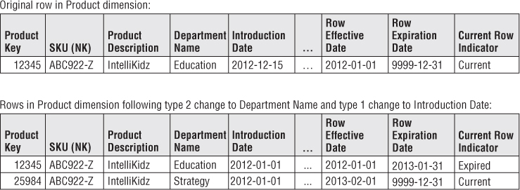
Using the type 2 approach, when IntelliKidz's department changed on February 1, 2013, a new product dimension row for IntelliKidz is inserted to reflect the new department attribute value. There are two product dimension rows for IntelliKidz, as illustrated in Figure 5.6. Each row contains a version of IntelliKidz's attribute profile that was true for a span of time.

Figure 5.6 SCD type 2 sample rows.

With type 2 changes, the fact table is again untouched; you don't go back to the historical fact table rows to modify the product key. In the fact table, rows for IntelliKidz prior to February 1, 2013, would reference product key 12345 when the product rolled up to the Education department. After February 1, new IntelliKidz fact rows would have product key 25984 to reflect the move to the Strategy department. This is why we say type 2 responses perfectly partition or segment history to account for the change. Reports summarizing pre-February 1 facts look identical whether the report is generated before or after the type 2 change.

We want to reinforce that reported results may differ depending on whether attribute changes are handled as a type 1 or type 2. Let's presume the electronic retailer sells $500 of IntelliKidz software during January 2013, followed by a $100 sale in February 2013. If the department attribute is a type 1, the results from a query reporting January and February sales would indicate $600 under Strategy. Conversely, if the department name attribute is a type 2, the sales would be reported as $500 for the Education department and $100 for the Strategy department.

Unlike the type 1 approach, there is no need to revisit preexisting aggregation tables when using the type 2 technique. Likewise, OLAP cubes do not need to be reprocessed if hierarchical attributes are handled as type 2.

If you constrain on the department attribute, the two product profiles are differentiated. If you constrain on the product description, the query automatically fetches both IntelliKidz product dimension rows and automatically joins to the fact table for the complete product history. If you need to count the number of products correctly, then you would just use the SKU natural key attribute as the basis of the distinct count rather than the surrogate key; the natural key column becomes the glue that holds the separate type 2 rows for a single product together.

Type 2 is the safest response if the business is not absolutely certain about the SCD business rules for an attribute. As we'll discuss in the “Type 6: Add Type 1 Attributes to Type 2 Dimension” and “Type 7: Dual Type 1 and Type 2 Dimensions” sections later in the chapter, you can provide the illusion of a type 1 overwrite when an attribute has been handled with the type 2 response. The converse is not true. If you treat an attribute as type 1, reverting to type 2 retroactively requires significant effort to create new dimension rows and then appropriately rekey the fact table.

Type 2 Effective and Expiration Dates

When a dimension table includes type 2 attributes, you should include several administrative columns on each row, as shown in Figure 5.6. The effective and expiration dates refer to the moment when the row's attribute values become valid or invalid. Effective and expiration dates or date/time stamps are necessary in the ETL system because it needs to know which surrogate key is valid when loading historical fact rows. The effective and expiration dates support precise time slicing of the dimension; however, there is no need to constrain on these dates in the dimension table to get the right answer from the fact table. The row effective date is the first date the descriptive profile is valid. When a new product is first loaded in the dimension table, the expiration date is set to December 31, 9999. By avoiding a null in the expiration date, you can reliably use a BETWEEN command to find the dimension rows that were in effect on a certain date.

When a new profile row is added to the dimension to capture a type 2 attribute change, the previous row is expired. We typically suggest the end date on the old row should be just prior to the effective date of the new row leaving no gaps between these effective and expiration dates. The definition of “just prior” depends on the grain of the changes being tracked. Typically, the effective and expiration dates represent changes that occur during a day; if you're tracking more granular changes, you'd use a date/time stamp instead. In this case, you may elect to apply different business rules, such as setting the row expiration date exactly equal to the effective date of the next row. This would require logic such as “>= effective date and < expiration date” constraints, invalidating the use of BETWEEN.

Some argue that a single effective date is adequate, but this makes for more complicated searches to locate the dimension row with the latest effective date that is less than or equal to a date filter. Storing an explicit second date simplifies the query processing. Likewise, a current row indicator is another useful administrative dimension attribute to quickly constrain queries to only the current profiles.

The type 2 response to slowly changing dimensions requires the use of surrogate keys, but you're already using them anyhow, right? You certainly can't use the operational natural key because there are multiple profile versions for the same natural key. It is not sufficient to use the natural key with two or three version digits because you'd be vulnerable to the entire list of potential operational issues discussed in Chapter 3. Likewise, it is inadvisable to append an effective date to the otherwise primary key of the dimension table to uniquely identify each version. With the type 2 response, you create a new dimension row with a new single-column primary key to uniquely identify the new product profile. This single-column primary key establishes the linkage between the fact and dimension tables for a given set of product characteristics. There's no need to create a confusing secondary join based on the dimension row's effective or expiration dates.

We recognize some of you may be concerned about the administration of surrogate keys to support type 2 changes. In Chapter 19: ETL Subsystems and Techniques and Chapter 20: ETL System Design and Development Process and Tasks, we'll discuss a workflow for managing surrogate keys and accommodating type 2 changes in more detail.

Type 1 Attributes in Type 2 Dimensions

It is not uncommon to mix multiple slowly changing dimension techniques within the same dimension. When type 1 and type 2 are both used in a dimension, sometimes a type 1 attribute change necessitates updating multiple dimension rows. Let's presume the dimension table includes a product introduction date. If this attribute is corrected using type 1 logic after a type 2 change to another attribute occurs, the introduction date should probably be updated on both versions of IntelliKidz's profile, as illustrated in Figure 5.7.

Figure 5.7 Type 1 updates in a dimension with type 2 attributes sample rows.

The data stewards need to be involved in defining the ETL business rules in scenarios like this. Although the DW/BI team can facilitate discussion regarding proper update handling, the business's data stewards should make the final determination, not the DW/BI team.

Type 3: Add New Attribute

Although the type 2 response partitions history, it does not enable you to associate the new attribute value with old fact history or vice versa. With the type 2 response, when you constrain the department attribute to Strategy, you see only IntelliKidz facts from after February 1, 2013. In most cases, this is exactly what you want.

However, sometimes you want to see fact data as if the change never occurred. This happens most frequently with sales force reorganizations. District boundaries may be redrawn, but some users still want the ability to roll up recent sales for the prior districts just to see how they would have done under the old organizational structure. For a few transitional months, there may be a need to track history for the new districts and conversely to track new fact data in terms of old district boundaries. A type 2 response won't support this requirement, but type 3 comes to the rescue.

In our software example, let's assume there is a legitimate business need to track both the new and prior values of the department attribute for a period of time around the February 1 change. With a type 3 response, you do not issue a new dimension row, but rather add a new column to capture the attribute change, as illustrated in Figure 5.8. You would alter the product dimension table to add a prior department attribute, and populate this new column with the existing department value (Education). The original department attribute is treated as a type 1 where you overwrite to reflect the current value (Strategy). All existing reports and queries immediately switch over to the new department description, but you can still report on the old department value by querying on the prior department attribute.

Figure 5.8 SCD type 3 sample rows.

Don't be fooled into thinking the higher type number associated with type 3 indicates it is the preferred approach; the techniques have not been presented in good, better, and best practice sequence. Frankly, type 3 is infrequently used. It is appropriate when there's a strong need to support two views of the world simultaneously. Type 3 is distinguished from type 2 because the pair of current and prior attribute values are regarded as true at the same time.

Type 3 is not useful for attributes that change unpredictably, such as a customer's home state. There would be no benefit in reporting facts based on a prior home state attribute that reflects a change from 10 days ago for some customers or 10 years ago for others. These unpredictable changes are typically handled best with type 2 instead.

Type 3 is most appropriate when there's a significant change impacting many rows in the dimension table, such as a product line or sales force reorganization. These en masse changes are prime candidates because business users often want the ability to analyze performance metrics using either the pre- or post-hierarchy reorganization for a period of time. With type 3 changes, the prior column is labeled to distinctly represent the prechanged grouping, such as 2012 department or pre-merger department. These column names provide clarity, but there may be unwanted ripples in the BI layer.

Finally, if the type 3 attribute represents a hierarchical rollup level within the dimension, then as discussed with type 1, the type 3 update and additional column would likely cause OLAP cubes to be reprocessed.

Multiple Type 3 Attributes

If a dimension attribute changes with a predictable rhythm, sometimes the business wants to summarize performance metrics based on any of the historic attribute values. Imagine the product line is recategorized at the start of every year and the business wants to look at multiple years of historic facts based on the department assignment for the current year or any prior year.

In this case, we take advantage of the regular, predictable nature of these changes by generalizing the type 3 approach to a series of type 3 dimension attributes, as illustrated in Figure 5.9. On every dimension row, there is a current department attribute that is overwritten, plus attributes for each annual designation, such as 2012 department. Business users can roll up the facts with any of the department assignments. If a product were introduced in 2013, the department attributes for 2012 and 2011 would contain Not Applicable values.

Figure 5.9 Dimension table with multiple SCD type 3 attributes.

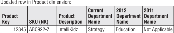
The most recent assignment column should be identified as the current department. This attribute will be used most frequently; you don't want to modify existing queries and reports to accommodate next year's change. When the departments are reassigned in January 2014, you'd alter the table to add a 2013 department attribute, populate this column with the current department values, and then overwrite the current attribute with the 2014 department assignment.

Type 4: Add Mini-Dimension

Thus far we've focused on slow evolutionary changes to dimension tables. What happens when the rate of change speeds up, especially within a large multimillion-row dimension table? Large dimensions present two challenges that warrant special treatment. The size of these dimensions can negatively impact browsing and query filtering performance. Plus our tried-and-true type 2 technique for change tracking is unappealing because we don't want to add more rows to a dimension that already has millions of rows, particularly if changes happen frequently.

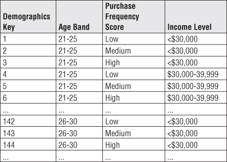
Fortunately, a single technique comes to the rescue to address both the browsing performance and change tracking challenges. The solution is to break off frequently analyzed or frequently changing attributes into a separate dimension, referred to as a mini-dimension. For example, you could create a mini-dimension for a group of more volatile customer demographic attributes, such as age, purchase frequency score, and income level, presuming these columns are used extensively and changes to these attributes are important to the business. There would be one row in the mini-dimension for each unique combination of age, purchase frequency score, and income level encountered in the data, not one row per customer. With this approach, the mini-dimension becomes a set of demographic profiles. Although the number of rows in the customer dimension may be in the millions, the number of mini-dimension rows should be a significantly smaller. You leave behind the more constant attributes in the original multimillion-row customer table.

Sample rows for a demographic mini-dimension are illustrated in Figure 5.10. When creating the mini-dimension, continuously variable attributes, such as income, are converted to banded ranges. In other words, the attributes in the mini-dimension are typically forced to take on a relatively small number of discrete values. Although this restricts use to a set of predefined bands, it drastically reduces the number of combinations in the mini-dimension. If you stored income at a specific dollar and cents value in the mini-dimension, when combined with the other demographic attributes, you could end up with as many rows in the mini-dimension as in the customer dimension itself. The use of band ranges is probably the most significant compromise associated with the mini-dimension technique. Although grouping facts from multiple band values is viable, changing to more discreet bands (such as $30,000-34,999) at a later time is difficult. If users insist on access to a specific raw data value, such as a credit bureau score that is updated monthly, it should be included in the fact table, in addition to being value banded in the demographic mini-dimension. In Chapter 10: Financial Services, we'll discuss dynamic value banding of facts; however, such queries are much less efficient than constraining the value band in a mini-dimension table.

Figure 5.10 SCD type 4 mini-dimension sample rows.

Every time a fact table row is built, two foreign keys related to the customer would be included: the customer dimension key and the mini-dimension demographics key in effect at the time of the event, as shown in Figure 5.11. The mini-dimension delivers performance benefits by providing a smaller point of entry to the facts. Queries can avoid the huge customer dimension table unless attributes from that table are constrained or used as report labels.

Figure 5.11 Type 4 mini-dimension with customer dimension.

When the mini-dimension key participates as a foreign key in the fact table, another benefit is that the fact table captures the demographic profile changes. Let's presume we are loading data into a periodic snapshot fact table on a monthly basis. Referring back to our sample demographic mini-dimension sample rows in Figure 5.10, if one of our customers, John Smith, were 25 years old with a low purchase frequency score and an income of $25,000, you'd begin by assigning demographics key 1 when loading the fact table. If John has a birthday several weeks later and turns 26 years old, you'd assign demographics key 142 when the fact table was next loaded; the demographics key on John's earlier fact table rows would not be changed. In this manner, the fact table tracks the age change. You'd continue to assign demographics key 142 when the fact table is loaded until there's another change in John's demographic profile. If John receives a raise to $32,000 several months later, a new demographics key would be reflected in the next fact table load. Again, the earlier rows would be unchanged. OLAP cubes also readily accommodate type 4 mini-dimensions.

Customer dimensions are somewhat unique in that customer attributes frequently are queried independently from the fact table. For example, users may want to know how many customers live in Dade County by age bracket for segmentation and profiling. Rather than forcing any analysis that combines customer and demographic data to link through the fact table, the most recent value of the demographics key also can exist as a foreign key on the customer dimension table. We'll further describe this customer demographic outrigger as an SCD type 5 in the next section.

The demographic dimension cannot be allowed to grow too large. If you have five demographic attributes, each with 10 possible values, then the demographics dimension could have 100,000 (10⁵) rows. This is a reasonable upper limit for the number of rows in a mini-dimension if you build out all the possible combinations in advance. An alternate ETL approach is to build only the mini-dimension rows that actually occur in the data. However, there are certainly cases where even this approach doesn't help and you need to support more than five demographic attributes with 10 values each. We'll discuss the use of multiple mini-dimensions associated with a single fact table in Chapter 10.

Demographic profile changes sometimes occur outside a business event, such as when a customer's profile is updated in the absence of a sales transaction. If the business requires accurate point-in-time profiling, a supplemental factless fact table with effective and expiration dates can capture every relationship change between the customer and demographics dimensions.

Hybrid Slowly Changing Dimension Techniques

In this final section, we'll discuss hybrid approaches that combine the basic SCD techniques. Designers sometimes become enamored with these hybrids because they seem to provide the best of all worlds. However, the price paid for greater analytic flexibility is often greater complexity. Although IT professionals may be impressed by elegant flexibility, business users may be just as easily turned off by complexity. You should not pursue these options unless the business agrees they are needed to address their requirements.

These final approaches are most relevant if you've been asked to preserve the historically accurate dimension attribute associated with a fact event, while supporting the option to report historical facts according to the current attribute values. The basic slowly changing dimension techniques do not enable this requirement easily on their own.

We'll start by considering a technique that combines type 4 with a type 1 outrigger; because 4 + 1 = 5, we're calling this type 5. Next, we'll describe type 6, which combines types 1 through 3 for a single dimension attribute; it's aptly named type 6 because 2 + 3 + 1 or 2 × 3 × 1 both equal 6. Finally, we'll finish up with type 7, which just happens to be the next available sequence number; there is no underlying mathematical significance to this label.

Type 5: Mini-Dimension and Type 1 Outrigger

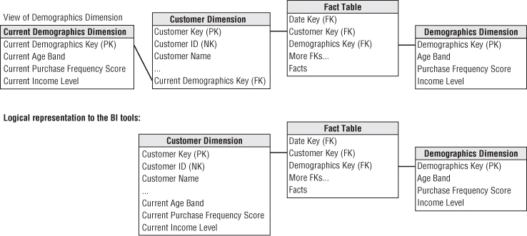
Let's return to the type 4 mini-dimension. An embellishment to this technique is to add a current mini-dimension key as an attribute in the primary dimension. This mini-dimension key reference is a type 1 attribute, overwritten with every profile change. You wouldn't want to track this attribute as a type 2 because then you'd be capturing volatile changes within the large multimillion-row dimension and avoiding this explosive growth was one of the original motivations for type 4.

The type 5 technique is useful if you want a current profile count in the absence of fact table metrics or want to roll up historical facts based on the customer's current profile. You'd logically represent the primary dimension and mini-dimension outrigger as a single table in the presentation area, as shown in Figure 5.12. To minimize user confusion and potential error, the current attributes in this role-playing dimension should have distinct column names distinguishing them, such as current age band. Even with unique labeling, be aware that presenting users with two avenues for accessing demographic data, through either the mini-dimension or outrigger, can deliver more functionality and complexity than some can handle.

Figure 5.12 Type 4 mini-dimension with type 1 outrigger in customer dimension.

Type 6: Add Type 1 Attributes to Type 2 Dimension

Let's return to the electronics retailer's product dimension. With type 6, you would have two department attributes on each row. The current department column represents the current assignment; the historic department column is a type 2 attribute representing the historically accurate department value.

When IntelliKidz software is introduced, the product dimension row would look like the first scenario in Figure 5.13.

Figure 5.13 SCD type 6 sample rows.

When the departments are restructured and IntelliKidz is moved to the Strategy department, you'd use a type 2 response to capture the attribute change by issuing a new row. In this new IntelliKidz dimension row, the current department will be identical to the historical department. For all previous instances of IntelliKidz dimension rows, the current department attribute will be overwritten to reflect the current structure. Both IntelliKidz rows would identify the Strategy department as the current department (refer to the second scenario in Figure 5.13).

In this manner you can use the historic attribute to group facts based on the attribute value that was in effect when the facts occurred. Meanwhile, the current attribute rolls up all the historical fact data for both product keys 12345 and 25984 into the current department assignment. If IntelliKidz were then moved into the Critical Thinking software department, the product table would look like Figure 5.13's final set of rows. The current column groups all facts by the current assignment, while the historic column preserves the historic assignments accurately and segments the facts accordingly.

With this hybrid approach, you issue a new row to capture the change (type 2) and add a new column to track the current assignment (type 3), where subsequent changes are handled as a type 1 response. An engineer at a technology company suggested we refer to this combo approach as type 6 because both the sum and product of 1, 2, and 3 equals 6.

Again, although this technique may be naturally appealing to some, it is important to always consider the business users' perspective as you strive to arrive at a reasonable balance between flexibility and complexity. You may want to limit which columns are exposed to some users so they're not overwhelmed by choices.

Type 7: Dual Type 1 and Type 2 Dimensions

When we first described type 6, someone asked if the technique would be appropriate for supporting both current and historic perspectives for 150 attributes in a large dimension table. That question sent us back to the drawing board.

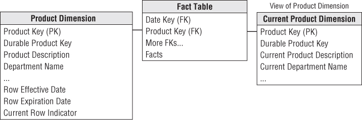
In this final hybrid technique, the dimension natural key (assuming it's durable) is included as a fact table foreign key, in addition to the surrogate key for type 2 tracking, as illustrated in Figure 5.14. If the natural key is unwieldy or ever reassigned, you should use a separate durable supernatural key instead. The type 2 dimension contains historically accurate attributes for filtering and grouping based on the effective values when the fact event occurred. The durable key joins to a dimension with just the current type 1 values. Again, the column labels in this table should be prefaced with “current” to reduce the risk of user confusion. You can use these dimension attributes to summarize or filter facts based on the current profile, regardless of the attribute values in effect when the fact event occurred.

Figure 5.14 Type 7 with dual foreign keys for dual type 1 and type 2 dimension tables.

This approach delivers the same functionality as type 6. Although the type 6 response spawns more attribute columns in a single dimension table, this approach relies on two foreign keys in the fact table. Type 7 invariably requires less ETL effort because the current type 1 attribute table could easily be delivered via a view of the type 2 dimension table, limited to the most current rows. The incremental cost of this final technique is the additional column carried in the fact table; however, queries based on current attribute values would be filtering on a smaller dimension table than previously described with type 6.

Of course, you could avoid storing the durable key in the fact table by joining the type 1 view containing current attributes to the durable key in the type 2 dimension table itself. In this case, however, queries that are only interested in current rollups would need to traverse from the type 1 outrigger through the more voluminous type 2 dimension before finally reaching the facts, which would likely negatively impact query performance for current reporting.

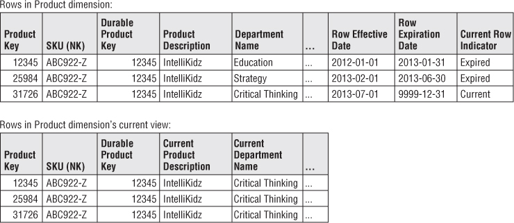
A variation of this dual type 1 and type 2 dimension table approach again relies on a view to deliver current type 1 attributes. However, in this case, the view associates the current attribute values with all the durable key's type 2 rows, as illustrated in Figure 5.15.

Figure 5.15 Type 7 variation with single surrogate key for dual type 1 and type 2 dimension tables.

Both dimension tables in Figure 5.15 have the same number of rows, but the contents of the tables are different, as shown in Figure 5.16.

Figure 5.16 SCD type 7 variation sample rows.

Type 7 for Random “As Of” Reporting

Finally, although it's uncommon, you might be asked to roll up historical facts based on any specific point-in-time profile, in addition to reporting by the attribute values in effect when the fact event occurred or by the attribute's current values. For example, perhaps the business wants to report three years of historical metrics based on the hierarchy in effect on December 1 of last year. In this case, you can use the dual dimension keys in the fact table to your advantage. First filter on the type 2 dimension row effective and expiration dates to locate the rows in effect on December 1 of last year. With this constraint, a single row for each durable key in the type 2 dimension is identified. Then join this filtered set to the durable key in the fact table to roll up any facts based on the point-in-time attribute values. It's as if you're defining the meaning of “current” on-the-fly. Obviously, you must filter on the row effective and expiration dates, or you'll have multiple type 2 rows for each durable key. Finally, only unveil this capability to a limited, highly analytic audience; this embellishment is not for the timid.

Slowly Changing Dimension Recap

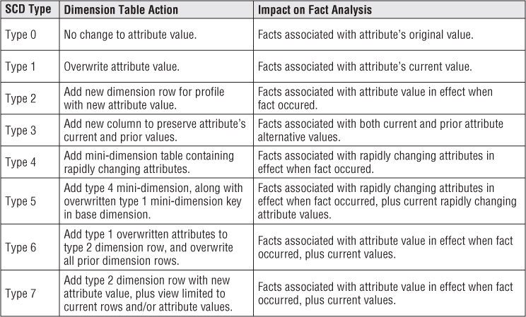
We've summarized the techniques for tracking dimension attribute changes in Figure 5.17. This chart highlights the implications of each slowly changing dimension technique on the analysis of performance metrics in the fact table.

Figure 5.17 Slowly changing dimension techniques summary.

Summary

In this chapter we discussed several approaches to handling procurement data. Effectively managing procurement performance can have a major impact on an organization's bottom line.

We also introduced techniques to deal with changes to dimension attribute values. The slowly changing responses range from doing nothing (type 0) to overwriting the value (type 1) to complicated hybrid approaches (such as types 5 through 7) which combine techniques to support requirements for both historic attribute preservation and current attribute reporting. You'll undoubtedly need to re-read this section as you consider slowly changing dimension attribute strategies for your DW/BI system.