
Chapter 2: Customizing Excel 2013
In This Chapter
![]() Customizing the Quick Access toolbar
Customizing the Quick Access toolbar
![]() Changing various and sundry Excel program settings
Changing various and sundry Excel program settings
![]() Extending Excel’s capabilities with add-in programs
Extending Excel’s capabilities with add-in programs
Chances are good that Excel 2013, as it comes right out of the box, is not always the best fit for the way you use the program. For that reason, Excel offers an amazing variety of ways to customize and configure the program’s settings so that they better suit your needs and the way you like to work.
This chapter covers the most important methods for customizing Excel settings and features. The chapter looks at three basic areas where you can tailor the program to your individual needs:
![]() The first place ripe for customization is the Quick Access toolbar. Not only can you control which Excel command buttons (on and off of the Ribbon) appear on this toolbar, but you can also assign macros you create to this toolbar, making them instantly accessible.
The first place ripe for customization is the Quick Access toolbar. Not only can you control which Excel command buttons (on and off of the Ribbon) appear on this toolbar, but you can also assign macros you create to this toolbar, making them instantly accessible.
![]() The second place where you may want to make extensive modifications is to the default settings (also referred to as options) that control any number of program assumptions and basic behaviors.
The second place where you may want to make extensive modifications is to the default settings (also referred to as options) that control any number of program assumptions and basic behaviors.
![]() The third place where you can customize Excel is in the world of add-ins, those small, specialized utilities (sometimes called applets) that extend the built-in Excel features by attaching themselves to the main Excel program. Excel add-ins provide a wide variety of functions and are available from a wide variety of sources, including the original Excel 2013 program, the Microsoft Office website, and various and sundry third-party vendors.
The third place where you can customize Excel is in the world of add-ins, those small, specialized utilities (sometimes called applets) that extend the built-in Excel features by attaching themselves to the main Excel program. Excel add-ins provide a wide variety of functions and are available from a wide variety of sources, including the original Excel 2013 program, the Microsoft Office website, and various and sundry third-party vendors.
Tailoring the Quick Access Toolbar to Your Tastes
Excel 2013 enables you to easily make modifications to the Quick Access toolbar, the sole toolbar remaining in this newest version of the program. When you first launch Excel, this toolbar appears above the Ribbon with the three most commonly used command buttons: Save, Undo, and Redo.
To add other commonly used commands to the Quick Access toolbar, such as New, Open, Email, Quick Print, and the like, simply click the Customize Quick Access toolbar button and choose this command from the drop-down menu.
 If you use Excel 2013 on a touchscreen device (such as the Microsoft Surface Tablet) the Touch/Mouse Mode button, which enables you to switch in and out of touch mode, is automatically added to the Quick Access toolbar. Touch mode puts more space between the command buttons on each tab of the Excel 2013 Ribbon, thus making it a whole lot easier to select the correct command with either your finger or stylus. Even when running Excel on a computer without any touch capabilities, you can still add the Touch/Mouse Mode button to the Quick Access toolbar and use touch mode to make it easier to select Tab commands with your mouse.
Adding Ribbon commands to the Quick Access toolbar
Excel 2013 makes it super-easy to add a command from any tab on the Ribbon to the Quick Access toolbar. To add a Ribbon command, simply right-click its command button on the Ribbon and then choose Add to Quick Access Toolbar from its shortcut menu. Excel immediately adds the command button to the very end of the Quick Access toolbar, immediately in front of the Customize Quick Access Toolbar button.
If you want to move the command button to a new location on the Quick Access toolbar or group it with other buttons on the toolbar, you need to click the Customize Quick Access Toolbar button and then choose More Commands from its drop-down menu.
Excel then opens the Excel Options dialog box with the Quick Access Toolbar tab selected (similar to the one shown in Figure 2-1). Here, Excel shows all the buttons currently added to the Quick Access toolbar in the order in which they appear from left to right on the toolbar corresponding to their top-down order in the list box on the right side of the dialog box.
To reposition a particular button on the bar, click it in the list box on the right and then click either the Move Up button (the one with the black triangle pointing upward) or the Move Down button (the one with the black triangle pointing downward) until the button is promoted or demoted to the desired position on the toolbar.

Figure 2-1: Use the buttons on the Quick Access Toolbar tab of the Excel Options dialog box to customize the appearance of the Quick Access toolbar.
 You can add separators to the toolbar to group related buttons. To do this, click the <Separator> selection in the list box on the left and then click the Add button twice to add two. Then, click the Move Up or Move Down button to position one of the two separators at the beginning of the group and the other at the end. Also keep in mind that you can always return the Quick Access toolbar to its default state with its three buttons (Save, Undo, and Redo) by selecting the Reset Only Quick Access Toolbar option from the Reset drop-down list.
If you’ve added too many buttons to the Quick Access toolbar and can no longer read the workbook name, you can reposition it so that it appears beneath the Ribbon immediately on top of the Formula bar. To do this, click the Customize Quick Access Toolbar button at the end of the toolbar and then choose Show Below the Ribbon from the drop-down menu.
Adding non-Ribbon commands to the Quick Access toolbar
You can also use the options on the Quick Access Toolbar tab of the Excel Options dialog box (refer to Figure 2-1) to add a button for any Excel command even if it’s not one of those displayed on the tabs of the Ribbon:
1. Select the type of command you want to add to the Quick Access toolbar from the Choose Commands From drop-down list box.
The types of commands include the default Popular Commands, Commands Not in the Ribbon, All Commands, and Macros, as well as each of the standard and contextual tabs that can appear on the Ribbon. To display only the commands not displayed on the Ribbon, select Commands Not in the Ribbon near the top of the drop-down list. To display a complete list of all the Excel commands, select All Commands near the bottom of the drop-down list.
2. Click the command option whose button you want to add to the Quick Access toolbar in the Choose Commands From list box on the left.
3. Click the Add button to add the command button to the bottom of the list box on the right.
4. (Optional) To reposition the newly added command button so that it’s not the last one on the toolbar, click the Move Up button until it’s in the desired position.
5. Click the OK button to close the Excel Options dialog box.
Adding macros to the Quick Access toolbar
If you’ve created favorite macros (see Book VIII, Chapter 1) that you routinely use and want to be able to run directly from the Quick Access toolbar, select Macros from the Choose Commands From drop-down list box and then click the name of the macro to add in the Choose Commands From list box followed by the Add button.
Adding commands lost from earlier Excel versions to the Quick Access toolbar
Although certain commands from earlier versions of Excel, such as Data⇒Form and Format⇒AutoFormat, did not make it to the Ribbon in Excel 2013, this does not mean that they were entirely eliminated from the program. The only way, however, to revive these commands is to add their command buttons to the Quick Access toolbar after selecting the Commands Not in the Ribbon category from the Choose Commands From drop-down list on the Customization tab of the Excel Options dialog box.
Excel 2013 then adds a custom macro command button to the end of the Quick Access toolbar whose generic icon displays the branching of a programming diagram. This means that if you add several favorite macros to the Quick Access toolbar, the only way to tell them apart is by their ScreenTips, each of which displays the location and name of the macro attached to the particular custom button when you highlight the button by passing the mouse pointer over it.
Exercising Your Options
Each time you open a new workbook, Excel makes a whole bunch of assumptions about how you want the spreadsheet and chart information that you enter into it to appear onscreen and in print. These assumptions may or may not fit the way you work and the kinds of spreadsheets and charts you need to create.
In the following five sections, you get a quick rundown on how to change the most important default or preference settings in the Excel Options dialog box. This is the biggest dialog box in Excel, with a billion tabs (ten actually). From the Excel Options dialog box, you can see what things appear onscreen and how they appear, as well as when and how Excel 2013 calculates worksheets.
Nothing discussed in the following five sections is critical to your being able to operate Excel. Just remember the Excel Options dialog box if you find yourself futzing with the same setting over and over again in most of the workbooks you create. In such a situation, it’s high time to get into the Excel Options dialog box and modify that setting so that you won’t waste any more time tinkering with the same setting in future workbooks.
Changing some of the more universal settings on the General tab
The General tab (shown in Figure 2-2) is the first tab in the Excel Options dialog box. This tab is automatically selected whenever you first open this dialog box by choosing File⇒Options or by pressing Alt+FT.
The options on the General tab are arranged into three groups: User Interface Options, When Creating New Workbooks, and Personalize Your Copy of Microsoft Office.
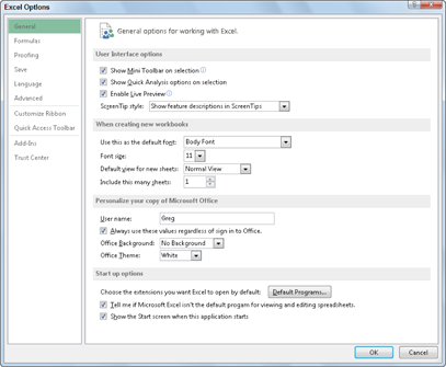
Figure 2-2: The General tab’s options enable you to change many universal Excel settings.
The User Interface Options group contains the following check boxes and buttons:
![]() Show Mini Toolbar on Selection: Disables or reenables the display of the mini-toolbar, which contains essential formatting buttons from the Home tab, above a cell selection or other object’s shortcut menu when you right-click it.
Show Mini Toolbar on Selection: Disables or reenables the display of the mini-toolbar, which contains essential formatting buttons from the Home tab, above a cell selection or other object’s shortcut menu when you right-click it.
![]() Show Quick Analysis Options on Selection: Disables or reenables the appearance of the new Quick Access toolbar in the lower-right corner of a cell selection. The Quick Analysis toolbar contains options for applying formatting to the selection as well as creating new charts and pivot tables using its data.
Show Quick Analysis Options on Selection: Disables or reenables the appearance of the new Quick Access toolbar in the lower-right corner of a cell selection. The Quick Analysis toolbar contains options for applying formatting to the selection as well as creating new charts and pivot tables using its data.
![]() Enable Live Preview: Disables or reenables the Live Preview feature whereby Excel previews the data in the current cell selection using the font or style you highlight in a drop-down list or gallery before you actually apply the formatting.
Enable Live Preview: Disables or reenables the Live Preview feature whereby Excel previews the data in the current cell selection using the font or style you highlight in a drop-down list or gallery before you actually apply the formatting.
![]() ScreenTip Style: Changes the way ScreenTips (that display information about the command buttons you highlight with the mouse) are displayed onscreen. Select Don’t Show Feature Descriptions in ScreenTips from the ScreenTip Style drop-down list to display a minimum amount of description in the ScreenTip and eliminate all links to online help, or select Don’t Show ScreenTips to completely remove the display of ScreenTips from the screen (potentially confusing if you add macros to the toolbar that all use the same icon).
ScreenTip Style: Changes the way ScreenTips (that display information about the command buttons you highlight with the mouse) are displayed onscreen. Select Don’t Show Feature Descriptions in ScreenTips from the ScreenTip Style drop-down list to display a minimum amount of description in the ScreenTip and eliminate all links to online help, or select Don’t Show ScreenTips to completely remove the display of ScreenTips from the screen (potentially confusing if you add macros to the toolbar that all use the same icon).
The options in the When Creating New Workbooks section of the Popular tab of the Excel Options dialog box include only these four combo and text boxes:
![]() Use This as the Default Font: Select a new default font to use in all cells of new worksheets by entering the font name in the combo box or selecting its name by clicking it in the drop-down list (Body Font, which is actually Microsoft’s Calibri font).
Use This as the Default Font: Select a new default font to use in all cells of new worksheets by entering the font name in the combo box or selecting its name by clicking it in the drop-down list (Body Font, which is actually Microsoft’s Calibri font).
![]() Font Size: Select a new default size to use in all cells of new worksheets (10 points is the default size for Excel running on Windows XP, and 11 points is the default size when running it on Windows Vista) by entering the value in the box, or select this new point value by clicking it in the drop-down list.
Font Size: Select a new default size to use in all cells of new worksheets (10 points is the default size for Excel running on Windows XP, and 11 points is the default size when running it on Windows Vista) by entering the value in the box, or select this new point value by clicking it in the drop-down list.
![]() Default View for New Sheets: Select either Page Break Preview (displaying page breaks that you can adjust) or Page Layout (displaying page breaks, rulers, and margins) as the default view (rather than Normal) for all new worksheets.
Default View for New Sheets: Select either Page Break Preview (displaying page breaks that you can adjust) or Page Layout (displaying page breaks, rulers, and margins) as the default view (rather than Normal) for all new worksheets.
![]() Include This Many Sheets: Increase or decrease the default number of worksheets in each new workbook (1 being the default) by entering a number between 2 and 225, or select this new number by clicking the spinner buttons.
Include This Many Sheets: Increase or decrease the default number of worksheets in each new workbook (1 being the default) by entering a number between 2 and 225, or select this new number by clicking the spinner buttons.
The Personalize Your Copy of Microsoft Office section contains the following three options:
![]() User Name: This text box enables you to change the user name that’s used as the default author for new workbooks created with Excel 2013.
User Name: This text box enables you to change the user name that’s used as the default author for new workbooks created with Excel 2013.
![]() Office Background: This drop-down list enables you to change the faint, background pattern that appears on the right side of the Excel title bar above the Ribbon. By default, the Clouds pattern appears as the background. To change this background pattern, select its name from the Office Background button’s drop-down list. To display no pattern in this area of the title bar, you select the None option from this drop-down list.
Office Background: This drop-down list enables you to change the faint, background pattern that appears on the right side of the Excel title bar above the Ribbon. By default, the Clouds pattern appears as the background. To change this background pattern, select its name from the Office Background button’s drop-down list. To display no pattern in this area of the title bar, you select the None option from this drop-down list.
![]() Office Theme: This drop-down list enables you to select between three different tint options — Dark Gray, Light Gray, and White — that are applied to the borders of the Excel screen, creating a kind of background color for the Ribbon tabs, column letter and row number indicators on the worksheet frame, and the status bar.
Office Theme: This drop-down list enables you to select between three different tint options — Dark Gray, Light Gray, and White — that are applied to the borders of the Excel screen, creating a kind of background color for the Ribbon tabs, column letter and row number indicators on the worksheet frame, and the status bar.
Remember that when the Always Use These Values Regardless of Sign In to Office check box in the Personalize Your Copy of Microsoft Office section is selected (as it is, by default), the user name, background pattern, and theme selected, respectively, for the User Name, Office Background, and Office Theme options are applied to all the Office 2013 application programs that you use, such as Word 2013, PowerPoint 2013, and so on.
The final section, Start Up Options, contains the following three options:
![]() Choose the Extensions You Want Excel to Open by Default: The Default Programs button, when clicked, opens a Set Associations for Program dialog box that enables you to select all the types of application files that you want associated with Excel 2013. Once associated with Excel, double-clicking any file carrying its extension automatically launches Excel 2013 for viewing and editing.
Choose the Extensions You Want Excel to Open by Default: The Default Programs button, when clicked, opens a Set Associations for Program dialog box that enables you to select all the types of application files that you want associated with Excel 2013. Once associated with Excel, double-clicking any file carrying its extension automatically launches Excel 2013 for viewing and editing.
![]() Tell Me if Microsoft Excel Isn’t the Default Program for Viewing and Editing Spreadsheets: This check box determines whether or not you’re informed should another Spreadsheet program or viewer on your computer other than Excel 2013 be associated with opening Excel workbook files.
Tell Me if Microsoft Excel Isn’t the Default Program for Viewing and Editing Spreadsheets: This check box determines whether or not you’re informed should another Spreadsheet program or viewer on your computer other than Excel 2013 be associated with opening Excel workbook files.
![]() Show the Start Screen When This Application Starts: This check box determines whether or not the Start screen (described in detail in Book I, Chapter 1) appears when you launch Excel 2013.
Show the Start Screen When This Application Starts: This check box determines whether or not the Start screen (described in detail in Book I, Chapter 1) appears when you launch Excel 2013.
If you deselect the Show the Start Screen When This Application Starts check box, whenever you launch Excel 2013, the program immediately opens a new, blank workbook file in the worksheet view, skipping entirely the Excel Backstage view. Excel 2013 then works just like Excel 2010 and 2007 on startup.
Changing common calculation options on the Formulas tab
The options on the Formulas tab (see Figure 2-3) of the Excel Options dialog box (File⇒Options⇒Formulas or Alt+FTF) are divided into Calculation Options, Working with Formulas, Error Checking, and Error Checking Rules.
The Calculation options enable you to change when formulas in your workbook are recalculated and whether and how a formula that Excel cannot solve on the first try (such as one with a circular reference) is recalculated. Choose from the following items:
![]() Automatic option button (the default) to have Excel recalculate all formulas immediately after you modify any of the values on which their calculation depends.
Automatic option button (the default) to have Excel recalculate all formulas immediately after you modify any of the values on which their calculation depends.
![]() Automatic Except for Data Tables option button to have Excel automatically recalculate all formulas except for those entered into what-if data tables you create. (See Book VII, Chapter 1.) To update these formulas, you must click the Calculate Now (F9) or the Calculate Sheet (Shift+F9) command button on the Formulas tab of the Ribbon.
Automatic Except for Data Tables option button to have Excel automatically recalculate all formulas except for those entered into what-if data tables you create. (See Book VII, Chapter 1.) To update these formulas, you must click the Calculate Now (F9) or the Calculate Sheet (Shift+F9) command button on the Formulas tab of the Ribbon.
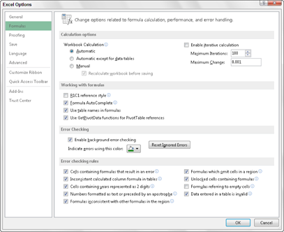
Figure 2-3: The Formulas tab’s options enable you to change how formulas in the spreadsheet are recalculated.
![]() Manual option button to switch to total manual recalculation, whereby formulas that need updating are recalculated only when you click the Calculate Now (F9) or the Calculate Sheet (Shift+F9) command button on the Formulas tab of the Ribbon.
Manual option button to switch to total manual recalculation, whereby formulas that need updating are recalculated only when you click the Calculate Now (F9) or the Calculate Sheet (Shift+F9) command button on the Formulas tab of the Ribbon.
![]() Enable Iterative Calculation check box to enable or disable iterative calculations for formulas that Excel finds that it cannot solve on the first try.
Enable Iterative Calculation check box to enable or disable iterative calculations for formulas that Excel finds that it cannot solve on the first try.
![]() Maximum Iterations text box to change the number of times (100 is the default) that Excel recalculates a seemingly insolvable formula when the Enable Iterative Calculation check box contains a check mark by entering a number between 1 and 32767 in the text box or by clicking the spinner buttons.
Maximum Iterations text box to change the number of times (100 is the default) that Excel recalculates a seemingly insolvable formula when the Enable Iterative Calculation check box contains a check mark by entering a number between 1 and 32767 in the text box or by clicking the spinner buttons.
![]() Maximum Change text box to change the amount by which Excel increments the guess value it applies each time the program recalculates the formula in an attempt to solve it by entering the new increment value in the text box.
Maximum Change text box to change the amount by which Excel increments the guess value it applies each time the program recalculates the formula in an attempt to solve it by entering the new increment value in the text box.
The Working with Formulas section contains four check box options that determine a variety of formula-related options:
![]() R1C1 Reference Style check box (unchecked by default) to enable or disable the R1C1 cell reference system whereby both columns and rows are numbered as in R45C2 for cell B45.
R1C1 Reference Style check box (unchecked by default) to enable or disable the R1C1 cell reference system whereby both columns and rows are numbered as in R45C2 for cell B45.
![]() Formula AutoComplete check box (checked by default) to disable or re-enable the Formula AutoComplete feature whereby Excel attempts to complete the formula or function you’re manually building in the current cell.
Formula AutoComplete check box (checked by default) to disable or re-enable the Formula AutoComplete feature whereby Excel attempts to complete the formula or function you’re manually building in the current cell.
![]() Use Table Names in Formulas check box (checked by default) to disable and reenable the feature whereby Excel automatically applies all range names you’ve created in a table of data to all formulas that refer to their cells. (See Book III, Chapter 1.)
Use Table Names in Formulas check box (checked by default) to disable and reenable the feature whereby Excel automatically applies all range names you’ve created in a table of data to all formulas that refer to their cells. (See Book III, Chapter 1.)
![]() Use GetPivotData Functions for PivotTable References check box (checked by default) to disable and reenable the GetPivotTable function that Excel uses to extract data from various fields in a data source when placing them in various fields of a pivot table summary report you’re creating. (See Book VII, Chapter 2 for details.)
Use GetPivotData Functions for PivotTable References check box (checked by default) to disable and reenable the GetPivotTable function that Excel uses to extract data from various fields in a data source when placing them in various fields of a pivot table summary report you’re creating. (See Book VII, Chapter 2 for details.)
The remaining options on the Formulas tab of the Excel Options dialog box enable you to control error-checking for formulas. In the Error Checking section, the sole check box, Enable Background Error Checking, which enables error-checking in the background while you’re working in Excel, is checked. In the Error Checking Rules, all of the check boxes are checked, with the exception of the Formulas Referring to Empty Cells check box, which indicates a formula error when a formula refers to a blank cell.
To disable background error checking, click the Enable Background Error Checking check box in the Error Checking section to remove its check mark. To change the color used to indicate formula errors in cells of the worksheet (when background error checking is engaged), click the Indicate Errors Using This Color drop-down button and click a new color square on its drop-down color palette. To remove the color from all cells in the worksheet where formula errors are currently indicated, click the Reset Ignore Errors button. To disable other error-checking rules, click their check boxes to remove the check marks.
Changing correction options on the Proofing tab
The options on the Proofing tab (see Figure 2-4) of the Excel Options dialog box (File⇒Options⇒Proofing or Alt+FTP) are divided into two sections: AutoCorrect Options and When Correcting Spelling in Microsoft Office Programs.
Click the AutoCorrect Options button to open the AutoCorrect dialog box for the primary language used in Microsoft Office 2013. This dialog box contains the following four tabs:
![]() AutoCorrect with check box options that control what corrections Excel automatically makes, an Exceptions button that enables you to indicate what words or abbreviations are not to be capitalized in the AutoCorrect Exceptions dialog box, and text boxes where you can define custom replacements that Excel makes as you type.
AutoCorrect with check box options that control what corrections Excel automatically makes, an Exceptions button that enables you to indicate what words or abbreviations are not to be capitalized in the AutoCorrect Exceptions dialog box, and text boxes where you can define custom replacements that Excel makes as you type.
![]() AutoFormat As You Type with check box options that control whether to replace Internet addresses and network paths with hyperlinks, and to automatically insert new rows and columns to cell ranges defined as tables and copy formulas in calculated fields to new rows of a data list.
AutoFormat As You Type with check box options that control whether to replace Internet addresses and network paths with hyperlinks, and to automatically insert new rows and columns to cell ranges defined as tables and copy formulas in calculated fields to new rows of a data list.
![]() Actions with an Enable Additional Actions in the Right-Click Menu check box and Available Actions list box that let you activate a date or financial symbol context menu that appears when you enter certain date and financial text in cells.
Actions with an Enable Additional Actions in the Right-Click Menu check box and Available Actions list box that let you activate a date or financial symbol context menu that appears when you enter certain date and financial text in cells.
![]() Math AutoCorrect with Replace and With text boxes that enable you to replace certain text with math symbols that are needed in your worksheets.
Math AutoCorrect with Replace and With text boxes that enable you to replace certain text with math symbols that are needed in your worksheets.
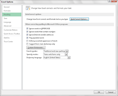
Figure 2-4: The Proofing tab’s options enable you to change AutoCorrect and spell-checking options.
The options in the When Correcting Spelling in Microsoft Office Programs section of the Proofing tab control what types of errors Excel flags as possible misspellings when you use the Spell Check feature. (See Book II, Chapter 3.) It also contains the following drop buttons:
![]() Custom Dictionaries, which opens the Custom Dictionaries dialog box, where you can specify a new custom dictionary to use in spell checking the worksheet, define a new dictionary, and edit its word list.
Custom Dictionaries, which opens the Custom Dictionaries dialog box, where you can specify a new custom dictionary to use in spell checking the worksheet, define a new dictionary, and edit its word list.
![]() French Modes or Spanish Modes, which specify which forms of the respective language to use in proofing spreadsheet text.
French Modes or Spanish Modes, which specify which forms of the respective language to use in proofing spreadsheet text.
![]() Dictionary Language, which specifies by language and country which dictionary to use in proofing spreadsheet text.
Dictionary Language, which specifies by language and country which dictionary to use in proofing spreadsheet text.
Changing various save options on the Save tab
The options on the Save tab (see Figure 2-5) of the Excel Options dialog box (File⇒Options⇒Save or Alt+FTS) are divided into four sections: Save Workbooks, AutoRecover Exceptions for the current workbook (such as Book1), Offline Editing Options for Document Management Server Files, and Preserve Visual Appearance of the Workbook.
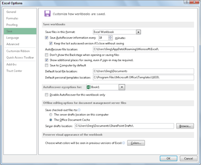
Figure 2-5: The Save tab’s options enable you to change the automatic backup and recover options.
The settings in the Save Workbooks section on this tab include the program’s AutoRecover settings. The AutoRecover feature enables Excel to save copies of your entire Excel workbook at the interval displayed in the Minutes text box (10 by default). You tell Excel where to save these copies in the AutoRecover File Location text box by specifying a drive, a folder, and maybe even a subfolder.
If your computer should crash or you suddenly lose power, the next time you start Excel the program automatically displays an AutoRecover pane. From this pane, you can open a copy of the workbook file that you were working on when this crash or power loss occurred. If this recovered workbook (saved at the time of the last AutoRecover) contains information that isn’t saved in the original copy (the copy you saved the last time you used the Save command before the crash or power loss), you can then use the recovered copy rather than manually reconstructing and reentering the otherwise lost information.
You may also use the recovered copy of a workbook should the original copy of the workbook file become corrupted in such a way that Excel can no longer open it. (This happens very rarely, but it does happen.)
 Don’t disable the AutoRecover feature by selecting the Disable AutoRecover for This Workbook Only check box on the Save tab even if you have a battery backup system for your computer that gives you plenty of time to manually save your Excel workbook during any power outage. Disabling AutoRecover in no way protects you from data loss if your workbook file becomes corrupted or you hit the computer’s power switch by mistake.
Beneath the AutoRecover File Location text box, you find the following Save Workbook options:
![]() Don’t Show the Backstage when Opening or Saving Files: Normally, Excel 2013 shows the Open screen in the Backstage view whenever you press Ctrl+O to open a file for editing and the Save As screen when you press Ctrl+S or select the Save button on the Quick Access toolbar to save a new workbook. Select this check box if you want Excel to display the Open and Save Dialog box in the Worksheet area (as was the case in previous versions of Excel) instead.
Don’t Show the Backstage when Opening or Saving Files: Normally, Excel 2013 shows the Open screen in the Backstage view whenever you press Ctrl+O to open a file for editing and the Save As screen when you press Ctrl+S or select the Save button on the Quick Access toolbar to save a new workbook. Select this check box if you want Excel to display the Open and Save Dialog box in the Worksheet area (as was the case in previous versions of Excel) instead.
![]() Show Additional Places for Saving, Even If Sign-in May Be Required: When Excel 2013 opens the Save As screen in the Backstage view, the program automatically displays the text boxes for logging into online services such as your SkyDrive or SharePoint team site on this screen. If you do not save your files to the Cloud or don’t have access to a SkyDrive, you can deselect this check box to remove such log-in options from the Save As screen.
Show Additional Places for Saving, Even If Sign-in May Be Required: When Excel 2013 opens the Save As screen in the Backstage view, the program automatically displays the text boxes for logging into online services such as your SkyDrive or SharePoint team site on this screen. If you do not save your files to the Cloud or don’t have access to a SkyDrive, you can deselect this check box to remove such log-in options from the Save As screen.
![]() Save to Computer by Default: If you prefer to save your workbook files locally on your computer’s hard drive or a virtual drive on a local area network to which you have access, select this check box.
Save to Computer by Default: If you prefer to save your workbook files locally on your computer’s hard drive or a virtual drive on a local area network to which you have access, select this check box.
![]() Default Local File Location: This text box contains the path to the local folder where Excel 2013 saves new workbook files by default when you select the Save to Computer by Default check box as described in the preceding bullet item.
Default Local File Location: This text box contains the path to the local folder where Excel 2013 saves new workbook files by default when you select the Save to Computer by Default check box as described in the preceding bullet item.
![]() Default Personal Templates Location: If the templates that you commonly use in creating new Excel workbooks are located in a local folder on your computer’s hard drive or a network drive to which you have access, enter the folder’s entire pathname in this text box after selecting the Save to Computer by Default check box as described earlier.
Default Personal Templates Location: If the templates that you commonly use in creating new Excel workbooks are located in a local folder on your computer’s hard drive or a network drive to which you have access, enter the folder’s entire pathname in this text box after selecting the Save to Computer by Default check box as described earlier.
If your company enables you to share the editing of certain Excel workbooks through the Excel Services offered as part of SharePoint Services software, you can change the location where Excel saves drafts of the workbook files you check out for editing. By default, Excel saves the drafts of these checked-out workbook files locally on your computer’s hard drive inside a SharePoint Drafts folder in the Documents (Windows 7 or Vista) or My Documents (Windows XP) folder. If your company or IT department prefers that you save these draft files on the web server that contains the SharePoint software, select the Office Document Cache option button to deselect The Server Drafts Location on This Computer option button and then enter the network path in the Server Drafts Location text box. Alternatively, click the Browse button and locate the network drive and folder in the Browse dialog box.
If you share your Excel 2013 workbooks with other less-fortunate workers who are still using older versions (97 through 2003) of Excel, use the Colors command button to determine which color in the Excel 2013 worksheet to preserve in formatted tables and other graphics when you save the workbook file for them using the Excel 97-2003 file format option. (See Book II, Chapter 1.)
Changing a whole lot of other common options on the Advanced tab
The options on the Advanced tab (see Figure 2-6) of the Excel Options dialog box (File⇒Options⇒Advanced or Alt+FTA) are divided into the 14 sections listed in the following table:
|
Option |
What It Does |
|
Editing Options |
Changes the way you edit the worksheets you create |
|
Cut, Copy, and Paste |
Changes the way worksheet editing involving cutting, copying, and pasting to and from the Clipboard works |
|
Image Size and Quality |
Controls how an image’s data is used in a worksheet |
|
|
Controls whether high or regular quality is used for the graphic images in the printed worksheet |
|
Chart |
Controls how Excel deals with the charts you add to a worksheet |
|
Display |
Determines how various elements (from recently used workbooks in the Backstage view to ruler units, the presence of the Formula bar, ScreenTips, and comments in the worksheet) appear onscreen |
|
Display Options for This Workbook |
Sets display options for the current workbook open in Excel |
|
Display Options for This Worksheet |
Sets display options for the currently selected worksheet in the workbook open in Excel |
|
Formulas |
Determines how Excel deals with calculating sophisticated formulas in the worksheets in your workbook |
|
When Calculating This Workbook |
Sets calculation parameters for the workbook open in Excel |
|
General |
Controls various all-purpose options, including such diverse options as the workbook files that you want opened when Excel launches, how your workbooks appear on the web, and the creation of custom AutoFill lists |
|
Data |
Controls how Excel copes with operations involving large amounts of data and the new Data Model |
|
Lotus Compatibility |
Sets general Lotus 1-2-3 compatibility in Excel 2013 |
|
Lotus Compatibility Settings |
Sets Lotus 1-2-3 compatibility for a particular worksheet in the workbook open in Excel |
The various and sundry options in these 14 sections of the Advanced tab actually fall into 4 somewhat distinct areas: options for editing in the worksheet; options controlling the screen display; a potpourri area of formulas, calculating, and general options; and Lotus compatibility options for old Lotus 1-2-3 users (assuming that there are still some of you left) who are just now upgrading to Excel to make the transition easier.
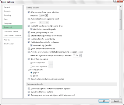
Figure 2-6: The Editing and Cut, Copy, and Paste options on the Advanced tab control how Excel behaves during editing.
Working the worksheet editing options
As you can see in Figure 2-6, the options in the Editing Options and Cut, Copy, and Paste sections on the Advanced tab control what happens when you edit the contents of an Excel worksheet.
When you first open the Advanced tab of the Excel Options dialog box, all of the check box options in the Editing Options and Cut, Copy, and Paste sections are checked with the exception of these three:
![]() Automatically Insert a Decimal Point to have Excel add a decimal point during data entry of all values in each worksheet using the number of places in the Places text box. (See Book II, Chapter 1 for details.)
Automatically Insert a Decimal Point to have Excel add a decimal point during data entry of all values in each worksheet using the number of places in the Places text box. (See Book II, Chapter 1 for details.)
![]() Zoom on Roll with IntelliMouse to have Excel increase or decrease the screen magnification percentage by 15 percent on each roll forward and back of the center wheel of a mouse that supports Microsoft’s IntelliMouse technology. When this option is not checked, Excel scrolls the worksheet up and down on each roll forward and back of the center wheel.
Zoom on Roll with IntelliMouse to have Excel increase or decrease the screen magnification percentage by 15 percent on each roll forward and back of the center wheel of a mouse that supports Microsoft’s IntelliMouse technology. When this option is not checked, Excel scrolls the worksheet up and down on each roll forward and back of the center wheel.
![]() Do Not Automatically Hyperlink Screenshot to prevent Excel from automatically creating hyperlinks to any screenshots that you take of the Windows desktop using the Screenshot option on the Illustrations button’s drop-down list on the Insert tab. (See Book V, Chapter 2 for details.)
Do Not Automatically Hyperlink Screenshot to prevent Excel from automatically creating hyperlinks to any screenshots that you take of the Windows desktop using the Screenshot option on the Illustrations button’s drop-down list on the Insert tab. (See Book V, Chapter 2 for details.)
Most of the time, you’ll want to keep all the check box options in the Editing Options and Cut, Copy, and Paste sections checked. The only one of these you might want to disengage is the Use System Separators check box when you routinely create spreadsheets with financial figures expressed in foreign currency that don’t use the period (.) as the decimal point and the comma (,) as the thousands separator. After you remove the check mark from the Use System Separators check box, the Decimal Separator and Thousands Separator text boxes become active, and you can then enter the appropriate punctuation into these two boxes.
By default, Excel selects Down as the Direction setting when the After Pressing Enter, Move Selection check box option is checked. If you want Excel to automatically advance the cell cursor in another direction (Right, Up, or Left), select the direction from its drop-down list. If you don’t want Excel to move the cell cursor outside of the active cell upon completion of the entry (the same as clicking the Enter button on the Formula bar), click the After Pressing Enter, Move Selection check box to remove its check mark.
Playing around with the display options
The display options in the middle of the Advanced tab of the Excel Options dialog box (see Figure 2-7) fall into three categories: general Display options that affect the Excel program; Display Options for This Workbook that affect the current workbook; and Display Options for This Worksheet that affect the active sheet in the workbook.
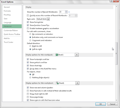
Figure 2-7: The various display options in the center of the Advanced tab control what’s shown on the screen.
Most of the options in these three categories are self-explanatory as they either turn off or on the display of particular screen elements such as the Formula bar, ScreenTips, scroll bars, sheet tabs, column and row headers, page breaks, (cell) gridlines, and the like.
When using these display options to control the display of various Excel screen elements, keep the following things in mind:
![]() The Ruler Units drop-down list box automatically uses the Default Units for your version of Microsoft Office (Inches in the U.S. and Centimeters in Europe). These default units (or those you specifically select from the drop-down list: Inches, Centimeters, or Millimeters) are then displayed on both the horizontal and vertical rulers that appear above and to the left of the column and row headings only when you put the Worksheet area display into Page Layout view (Alt+WP).
The Ruler Units drop-down list box automatically uses the Default Units for your version of Microsoft Office (Inches in the U.S. and Centimeters in Europe). These default units (or those you specifically select from the drop-down list: Inches, Centimeters, or Millimeters) are then displayed on both the horizontal and vertical rulers that appear above and to the left of the column and row headings only when you put the Worksheet area display into Page Layout view (Alt+WP).
![]() Click the Comments and Indicators option button under the For Cells with Comments, Show heading when you want Excel to display the text boxes with the comments you add to cells at all times in the worksheet. (See Book IV, Chapter 3.)
Click the Comments and Indicators option button under the For Cells with Comments, Show heading when you want Excel to display the text boxes with the comments you add to cells at all times in the worksheet. (See Book IV, Chapter 3.)
![]() Click the Nothing (Hide Objects) option button under the For Objects, Show heading when you want Excel to hide the display of all graphic objects in the worksheet, including embedded charts, clip art, imported pictures, and all graphics that you generate in the worksheet. (See Book V, Chapters 1 and 2 for details.)
Click the Nothing (Hide Objects) option button under the For Objects, Show heading when you want Excel to hide the display of all graphic objects in the worksheet, including embedded charts, clip art, imported pictures, and all graphics that you generate in the worksheet. (See Book V, Chapters 1 and 2 for details.)
![]() Click the Show Page Breaks check box to remove its check mark whenever you need to remove the dotted lines indicating page breaks in Normal (Alt+WN) view after viewing the Worksheet area in either Page Break Preview (Alt+WI) or Page Layout view (Alt+WP).
Click the Show Page Breaks check box to remove its check mark whenever you need to remove the dotted lines indicating page breaks in Normal (Alt+WN) view after viewing the Worksheet area in either Page Break Preview (Alt+WI) or Page Layout view (Alt+WP).
![]() Instead of going to the trouble of clicking the Show Formulas in Cells Instead of Their Calculated Results check box to display formulas in the cells of the worksheet, simply press Ctrl+’ (apostrophe) or click the Show Formulas button on the Formulas tab of the Ribbon. Both the keystroke shortcut and the button are toggles so that you can return the Worksheet area to its normal display showing the calculated results rather than the formulas by pressing the Ctrl+’ shortcut keys again or clicking the Show Formulas button.
Instead of going to the trouble of clicking the Show Formulas in Cells Instead of Their Calculated Results check box to display formulas in the cells of the worksheet, simply press Ctrl+’ (apostrophe) or click the Show Formulas button on the Formulas tab of the Ribbon. Both the keystroke shortcut and the button are toggles so that you can return the Worksheet area to its normal display showing the calculated results rather than the formulas by pressing the Ctrl+’ shortcut keys again or clicking the Show Formulas button.
![]() Instead of going to the trouble of removing the check mark from the Show Gridlines check box whenever you want to remove the column and row lines that define the cells in the Worksheet area, click the Gridlines check box in the Show/Hide group on the View tab or the View check box in the Gridlines column of the Sheet Options group on the Page Layout tab to remove their check marks.
Instead of going to the trouble of removing the check mark from the Show Gridlines check box whenever you want to remove the column and row lines that define the cells in the Worksheet area, click the Gridlines check box in the Show/Hide group on the View tab or the View check box in the Gridlines column of the Sheet Options group on the Page Layout tab to remove their check marks.
Use the Gridline Color drop-down list button immediately below the Show Gridlines check box to change the color of the Worksheet gridlines (when they’re displayed, of course) by clicking a new color on the color palette that appears when you click its drop-down list button. (I find that navy blue makes the cell boundaries stand out particularly well and gives the screen a hint of the old paper green-sheet look.)
Caring about the Formulas, Calculating, and General options
At the bottom of the Advanced tab of the Excel Options dialog box (see Figure 2-8), you find a regular mix of options in five sections. The first three sections, Formulas, When Calculating This Workbook, and General, contain a veritable potpourri of options.
The settings of most of the options in these three sections won’t need changing. In rare cases, you may find that you have to activate the following options or make modifications to some of their settings:
![]() Set Precision as Displayed: Select this check box only when you want to permanently change the calculated values in the worksheet to the number of places currently shown in their cells as the result of the number format applied to them.
Set Precision as Displayed: Select this check box only when you want to permanently change the calculated values in the worksheet to the number of places currently shown in their cells as the result of the number format applied to them.

Figure 2-8: The options at the bottom of the Advanced tab control various calculation, general, data, and 1-2-3 compatibility settings.
![]() Use 1904 Date System: Select this check box when you’re dealing with a worksheet created with an earlier Macintosh version of Excel that used 1904 rather than 1900 as date serial number 1.
Use 1904 Date System: Select this check box when you’re dealing with a worksheet created with an earlier Macintosh version of Excel that used 1904 rather than 1900 as date serial number 1.
![]() Web Options: Click this command button to display the Web Options dialog box, where you can modify the options that control how your Excel data appears when viewed with a web browser, such as Internet Explorer.
Web Options: Click this command button to display the Web Options dialog box, where you can modify the options that control how your Excel data appears when viewed with a web browser, such as Internet Explorer.
![]() Edit Custom Lists: Click this command button to create or edit custom lists with the Fill handle. (See Book II, Chapter 1.)
Edit Custom Lists: Click this command button to create or edit custom lists with the Fill handle. (See Book II, Chapter 1.)
Digging the Data options
The Advanced tab of the Excel Options dialog box now contains a new section called Data with three check box options. These options control the way that Excel 2013 handles huge amounts of data that you can access in Excel through external data queries discussed in Book VI, Chapter 2 or through Excel’s pivot table feature (especially when using the Power Pivot add-in) discussed Book VII, Chapter 2.
By default, Excel 2013 disables the undo feature when refreshing data in a pivot table created from external data that has more than 300,000 source rows (also called records) to significantly reduce the data refresh time. To modify the minimum number of source rows at which the undo refresh feature is disabled, enter a new number (representing thousands of records) in the text box containing the default value of 300 under the Disable Undo for Large PivotTable Refresh Operations check box or select the new value with the spinner buttons. To enable the undo feature for all refresh operations in your large pivot tables (regardless of how long the refresh operation takes), simply deselect the Disable Undo for Large PivotTable Refresh Operations check box.
Excel 2013 also automatically disables the undo feature for Excel data lists that are created from related external database tables (referred to in Excel as a data model) that exceed 64MB in size. To change the minimum size at which the undo feature is disabled, enter a new number (representing megabytes) in the text box containing the default value of 64 under the Disable Undo for Large Data Model Operations check box or select this new value with the spinner buttons. To enable the undo feature for all operations involving data lists created from an external data model (regardless of how long the undo operation takes), simply deselect the Disable Undo for Large Data Model Operations check box.
If you want Excel to automatically assume that any external data used in creating new pivot tables or imported into data lists from external data queries involve a data model so that Excel automatically looks for the fields that are related in the various files you designate, select the Prefer the Excel Data Model When Creating PivotTables, QueryTables and Data Connections check box in the Data section on the Advanced tab of the Excel Options dialog box.
Laying on the Lotus 1-2-3 compatibility
The last two sections on the Advanced tab, Lotus Compatibility and Lotus Compatibility Settings For, are only of interest to Lotus 1-2-3 users who are just now coming to use Microsoft Excel as their spreadsheet program.
If you’re a dyed-in-the-wool 1-2-3 user, you’ll definitely want to put a check mark in all three check boxes, Transition Navigation Keys, Transition Formula Evaluation, and Transition Formula Entry, in both the Lotus Compatibility and Lotus Compatibility Settings For sections. That way, you’ll be able to start formulas with built-in functions with the @ symbol — which Excel dutifully converts to an equal sign (=) — as well as use all the keys for navigating the worksheet to which you’ve become so accustomed.
Keep in mind that you can activate the hot keys on the Excel Ribbon by pressing the forward slash (/) key even when none of the Lotus compatibility options are selected. When I want to use the program’s hot keys to select an Excel command from the Ribbon, I find pressing the forward slash, which activated the pull-down menus in Lotus 1-2-3, to be much easier than pressing the Alt key — this is because / is part of the QWERTY keyboard. This means that whenever you see a keyboard shortcut such as Alt+WP in the book, you can just press /WP (which in this particular case puts the Worksheet display area into Page Layout view).
Customizing the Excel 2013 Ribbon
The options on the new Customize Ribbon tab (see Figure 2-9) of the Excel Options dialog box (File⇒Options⇒Customize Ribbon or Alt+FTC) enable you to modify which tabs appear on the Excel Ribbon and the order in which they appear, as well as to change which groups of command buttons appear on each of these displayed tabs. You can even use its options to create brand-new tabs for the Ribbon as well as create custom groups of command buttons within any of the displayed tabs.
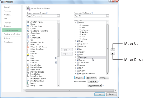
Figure 2-9: The Customize Ribbon tab options enable you to control which tabs are displayed on the Ribbon and which groups of command buttons they contain.
Customizing the Ribbon’s tabs
If you find that the default arrangement of main tabs and groups on the Excel Ribbon is not entirely to your liking, you can simplify or rearrange them to suit the way you routinely work:
![]() Hide tabs on the Ribbon by deselecting their check boxes in the Main Tabs list box on the right side of the Excel Options dialog box. (To later redisplay a hidden tab, you simply select its check box.)
Hide tabs on the Ribbon by deselecting their check boxes in the Main Tabs list box on the right side of the Excel Options dialog box. (To later redisplay a hidden tab, you simply select its check box.)
![]() Modify tab order on the Ribbon by selecting the tab to move and then click either the Move Up button (with the triangle pointing up) or Move Down button (the triangle pointing down) until the name of the tab appears in the desired position in list shown in the Main Tabs list box.
Modify tab order on the Ribbon by selecting the tab to move and then click either the Move Up button (with the triangle pointing up) or Move Down button (the triangle pointing down) until the name of the tab appears in the desired position in list shown in the Main Tabs list box.
![]() Modify group order on a tab by first expanding the tab to display the groups by clicking the Expand button (with the plus sign) in front of the tab name in the Main Tabs list box. Next click the name of the group you want to reposition and click either the Move Up or Move Down button until it appears in the desired position in the list.
Modify group order on a tab by first expanding the tab to display the groups by clicking the Expand button (with the plus sign) in front of the tab name in the Main Tabs list box. Next click the name of the group you want to reposition and click either the Move Up or Move Down button until it appears in the desired position in the list.
![]() Remove a group from a tab by selecting its name in the expanded Main Tabs list and then clicking the Remove command button (under the Add button between the two list boxes that now appear in the main section of the Excel Options dialog box).
Remove a group from a tab by selecting its name in the expanded Main Tabs list and then clicking the Remove command button (under the Add button between the two list boxes that now appear in the main section of the Excel Options dialog box).
In addition to the main tabs of the Ribbon, you can control which groups of command buttons appear on its various contextual tabs (such as the Drawing Tools or Chart Tools contextual tabs that automatically appear when you’re working on an Excel table of data or chart):
![]() Display the groups to be modified on a contextual tab by clicking the Tool Tabs option on the Customize the Ribbon drop-down list and then clicking the Expand button in front of the contextual tab whose groups you want to modify.
Display the groups to be modified on a contextual tab by clicking the Tool Tabs option on the Customize the Ribbon drop-down list and then clicking the Expand button in front of the contextual tab whose groups you want to modify.
![]() Modify the group order on a contextual tab by clicking the group name and then clicking the Move Up or Move Down buttons to move it into its new position.
Modify the group order on a contextual tab by clicking the group name and then clicking the Move Up or Move Down buttons to move it into its new position.
![]() Remove a group from a contextual tab by clicking its group name and then clicking the Remove command button.
Remove a group from a contextual tab by clicking its group name and then clicking the Remove command button.
To restore the original groups to a particular tab you’ve modified, select the tab in the Customize the Ribbon list box on the right side of the Excel Options dialog box and then click the Reset drop-down button beneath this list box before you select the Reset Only Selected Ribbon Tab option.
If you want to restore all the tabs and groups on the Ribbon to their original default arrangement, you can click the Reset drop-down button and then select the Reset All Customizations option from its drop-down list. Just be aware that selecting this option not only restores the Ribbon’s default settings but also negates all changes you’ve made to the Quick Access toolbar at the same time. If you don’t want this to happen, restore the tabs of the Ribbon individually by using the Reset Only Selected Ribbon tab option described in the preceding tip.
Adding custom tabs to the Ribbon
The Customize Ribbon tab of the Excel Options dialog box not only lets you customize the existing Ribbon tabs but also lets you add ones of your own. This is great news for you if you want Ribbon access to Excel commands you routinely rely on that didn’t make it to the default Ribbon.
To add a brand-new tab to the Ribbon, follow these steps:
1. Open the Customize Ribbon tab of the Excel Options dialog box (File⇒Options⇒Customize Ribbon or Alt+FTC).
Excel opens the Customize Ribbon tab with the Main Tabs selected in the Customize the Ribbon list box on the right.
2. Select the tab under Main Tabs in this list box immediately after which the new Ribbon is to be inserted.
By default, Excel inserts the new tab after the one that’s currently selected in the Customize the Ribbon list box. This means that if you want your new custom tab to precede the Home tab, you must put it ahead of the Home tab with the Move Up button after first creating the new tab behind it.
3. Click the New Tab command button below Main Tabs in the Customize the Ribbon list box.
Excel inserts a tab called New Tab (custom) with the single group called New Group (Custom) displayed and selected. This New Tab (Custom) is placed immediately after the currently selected tab.
4. Add all the commands you want in this group on the custom tab by selecting them in the Choose Commands From list box and then clicking the Add Command button.
When adding commands, you can select them from any of the categories: Popular Commands, Commands Not in the Ribbon, All Commands, Macros, Office Menu, All Tabs, Main Tabs, Tool Tabs, and Custom Tabs and Groups (which lists all custom tabs and groups you’ve previously created).
As you add each command from these categories, Excel displays the button’s icon and name in the list beneath New Group (Custom) in the left-to-right order in which they’ll appear. (See Figure 2-10.) To change the order of these command buttons in the new group on the custom tab, click the Move Up and/or Move Down buttons.
5. Rename the new group by clicking the Rename button under the Customize the Ribbon list box and then typing the new name in the Display Name text box of the Rename dialog box before clicking OK.
6. (Optional) To add other groups to the same custom tab, click the New Group button under the Customize the Ribbon list box and then add all its command buttons before renaming it. (Refer to Steps 4 and 5.)
To add any additional groups of commands to be included on the new custom tab, simply repeat Step 6. Use the Move Up and Move Down buttons if you need to reposition any groups on the custom tab.
7. Rename the custom tab by clicking the New Tab (Custom) in the Customize the Ribbon list box. Then, click Rename button and type the name for the tab in the Display Name text box of the Rename dialog box before you click OK.
To add additional custom tabs to the Ribbon, repeat Steps 2 through 7. After you finish all your custom tabs to the Ribbon, you’re ready to close the Excel Options dialog box and return to the worksheet.
8. Click the OK button in the Excel Options dialog box.
When Excel closes this dialog box and returns you to the worksheet, the new custom tab appears in the Ribbon at the position where you placed it.
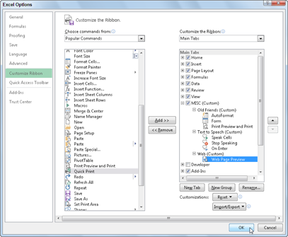
Figure 2-10: Adding forgotten Excel commands to a custom group on a brand new Ribbon tab.
Figure 2-11 shows you the Excel Ribbon on my computer after I added a Misc tab to the very end. As you can see, when this tab is selected it contains three custom groups: Old Friends (Custom) with AutoFormat, Form, and Print Preview and Print buttons; Text to Speech (Custom) with the Speak Cells, Stop Speaking, and On Enter buttons; and Web (Custom) with its Web Page Preview button.
If you use shortcut keys to access Ribbon commands, keep in mind that Excel automatically assigns hot-key letters to each of the custom tabs and commands you add to the Ribbon. To display the custom tabs’ hot keys, press the Alt key. To display the hot keys assigned to the commands on a particular custom tab, type its specific hot-key letter.
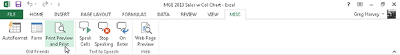
Figure 2-11: Excel Ribbon after selecting a Misc tab with its command buttons clustered in three custom groups.
Using Office Apps
Excel 2013 now supports the use of Office apps to help you build your worksheets. Office apps are small application programs that run within specific Office 2013 programs such as Excel and increase particular functionality to promote greater productivity.
There are Office apps to help you learn about Excel’s features, look up words in the Merriam-Webster dictionary, and even enter dates into your spreadsheet by selecting them on a calendar. Many of the Office apps for Excel 2013 are available free of charge, whereas others are offered for purchase from the Office Store for a small price.
To use any of these apps in Excel 2013, you first need to install them by following these steps:
1. Select the Apps for Office button on the Insert tab of the Ribbon.
The Apps for Office drop-down menu appears with a Recently Used Apps section at the top and a See All link at the bottom. The first time you open this menu, the Recently Used Apps section is blank.
2. Choose the See All option from the Apps for Office drop-down menu.
Excel opens the Apps for Office dialog box containing My Apps and Featured Apps links, along with an Editor’s Picks section and Recently Added section, each with its own free apps that you can install.
3. (Optional) Click the More Apps link in the Editor’s Picks section to go online and display a list of all the apps available for Excel 2013.
Excel opens the Apps for Excel 2013 page in the Office Store website that displays a list of all the apps currently available to install and use in Excel 2013. Each app in the list is identified by icon, name, its developer, its current user rating, and its price.
4. To get more information about a particular app, click its name or icon.
A page on the Microsoft Office Store’s website opens that gives you detailed information about the app you selected.
5. To install the app, click the Add button and then click the Continue button on the confirmation page.
When you click Add to install a free app, your browser takes you directly to a confirmation page followed by a page indicating how you insert the app in Excel. For apps you must purchase, your browser takes you to a page where you provide your account information. When the purchase is approved, your web browser takes you to the page telling you how to insert your app into Excel.
6. Click the Close button on your web browser to return to Excel.
After you complete the installation, you can then insert the apps you want to use into the current worksheet. To do this, follow these steps:
1. If the Apps for Office dialog box is not currently open in Excel, open it by choosing Insert⇒Apps for Office⇒See All or press Alt+NAPS.
2. Click the My Apps link in the App for Office dialog box.
Excel displays all the Office apps currently installed for Excel. (See Figure 2-12.)
3. Click the app you want to use in your worksheet to select it and then click the Insert button or press Enter.
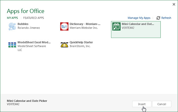
Figure 2-12: Inserting the Mini Calendar and Date Picker Office app into Excel.
Excel then inserts the app into your current worksheet so that you can start using its features. Some Office apps such as the Merriam-Webster Dictionary app and QuickHelp Starter open in task panes docked on the right side of the worksheet window. Others, such as Bing Maps and the Mini Calendar and Date Picker, open as graphic objects that float above the worksheet.
To close Office apps that open in docked task panes, you simply click the pane’s Close button. To close Office apps that open as floating graphic objects, you need to select the graphic and then press the Delete key. (Don’t worry — doing this only closes the app without uninstalling it.)
Note that after you start using various apps in Excel, they’re added to the Recently Used Apps section of the Apps for Office button’s drop-down menu. You can then quickly reopen any closed app that appears on this menu simply by clicking it.
If you don’t see any of your installed apps in the App for Office dialog box after clicking the My Apps link, click the Refresh link to Excel to refresh the list. Use the Manage My Apps link in this dialog box to keep tabs on all the apps you’ve installed for Office 2013 and SharePoint, as well as to uninstall any app that you’re no longer using.
Add-In Mania
Add-ins are small, specialized programs that extend Excel’s built-in features in some way. Most of the add-in programs created for Excel offer you some kind of specialized function or group of functions that extend Excel’s computational capabilities. Before you can use any add-in program, the add-in must be installed in the proper folder on your hard drive, and then you must select the add-in in the Add-Ins dialog box.
There are two different types of add-in programs immediately available that you can use to extend the features in Excel 2013:
![]() Excel Add-ins: This group of add-ins (also known as automation add-ins) is designed to extend the data analysis capabilities of Excel. These include Analysis ToolPak, Euro Currency Tools, and Solver.
Excel Add-ins: This group of add-ins (also known as automation add-ins) is designed to extend the data analysis capabilities of Excel. These include Analysis ToolPak, Euro Currency Tools, and Solver.
![]() COM Add-ins: COM (Component Object Model) add-ins are designed to extend Excel’s capability to deal with and analyze large amounts of data in data models (collections of related database tables). These include PowerPivot, Power View, and Inquire.
COM Add-ins: COM (Component Object Model) add-ins are designed to extend Excel’s capability to deal with and analyze large amounts of data in data models (collections of related database tables). These include PowerPivot, Power View, and Inquire.
When you first install Excel 2013, the add-in programs included with Excel are not loaded and therefore are not yet ready to use. To load any or all of these add-in programs, you follow these steps:
1. Click the File menu button, click Excel Options or press Alt+FT to open the Excel Options dialog box, and then click the Add-Ins tab.
The Add-Ins tab lists all the names, locations, and types of the add-ins to which you have access.
2. (Optional) In the Manage drop-down list box at the bottom, Excel Add-Ins is selected by default. If you want to activate one or more of your COM add-ins, select COM Add-Ins from the Manage drop-down list.
3. Select the Go button.
If Excel Add-Ins was selected in the Manage drop-down list box, Excel opens the Add-Ins dialog box (similar to the one shown in Figure 2-13), showing all the names of the built-in add-in programs you can load. If COM Add-Ins was selected, the COM Add-Ins dialog box appears instead.
4. Click the check boxes for each add-in program that you want loaded in the Add-Ins or COM Add-Ins dialog box.
Click the name of the add-in in the Add-Ins Available list box to display a brief description of its function at the bottom of this dialog box.
5. Click the OK button to close the Add-Ins or COM Add-Ins dialog box.
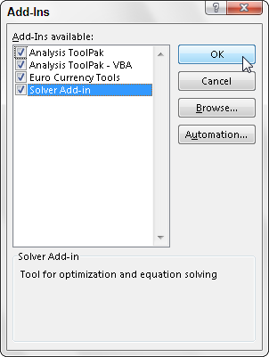
Figure 2-13: Activating built-in add-ins in the Add-Ins dialog box.
When you first install Excel 2013, the program automatically loads all four add-ins (Analysis ToolPak, Analysis ToolPak - VBA, Euro Currency Tools, and Solver Add-In) displayed in the Add-Ins Available list box. (For more about these add-ins, see the following section, “Managing Excel add-ins.”) The tools in the two Analysis ToolPaks are added as special functions to the Function Library group and the Euro Currency tools to a Solutions group on the Formulas tab. The Solver add-in appears in the Analysis group on the Data tab.
Excel add-in programs are saved in a special file format identified with the .XLA or .XLAM (for Excel Add-in) filename extension. These files are normally saved inside the Library folder (sometimes in their own subfolders) that is located in the Office14 folder. The Office14 folder, in turn, is located in your Microsoft Office folder inside the Program Files folder on your hard drive (often designated as the C: drive). In other words, the path is
c:Program FilesMicrosoft OfficeOffice14Library
After an add-in program has been installed in the Library folder, its name then appears in the list box of the Add-Ins dialog box.
If you ever copy an XLA add-in program to a folder other than the Library folder in the Office14 folder on your hard drive, its name won’t appear in the Add-Ins Available list box when you open the Add-Ins dialog box. You can, however, activate the add-in by clicking the Browse button in this dialog box and then selecting the add-in file in its folder in the Browse dialog box before you click OK.
Managing Excel add-ins
Whether you know it or not, you already have a group of add-in programs waiting for you to use. The following Excel add-in programs are loaded when you install Excel 2013:
![]() Analysis ToolPak: Adds extra financial, statistical, and engineering functions to Excel’s pool of built-in functions.
Analysis ToolPak: Adds extra financial, statistical, and engineering functions to Excel’s pool of built-in functions.
![]() Analysis ToolPak - VBA: Enables VBA programmers to publish their own financial, statistical, and engineering functions for Excel.
Analysis ToolPak - VBA: Enables VBA programmers to publish their own financial, statistical, and engineering functions for Excel.
![]() Euro Currency Tools: Enables you to format worksheet values as euro currency and adds a EUROCONVERT function for converting other currencies into euros. To use these tools, click the Euro Conversion or Euro Formatting buttons that appear on the Ribbon in the Solutions group at the end of the Formulas tab.
Euro Currency Tools: Enables you to format worksheet values as euro currency and adds a EUROCONVERT function for converting other currencies into euros. To use these tools, click the Euro Conversion or Euro Formatting buttons that appear on the Ribbon in the Solutions group at the end of the Formulas tab.
![]() Solver Add-In: Calculates solutions to what-if scenarios based on cells that both adjust and constrain the range of values. (See Book VII, Chapter 1.) To use the Solver add-in, click the Solver button that appears on the Ribbon in the Analysis group at the end of the Data tab.
Solver Add-In: Calculates solutions to what-if scenarios based on cells that both adjust and constrain the range of values. (See Book VII, Chapter 1.) To use the Solver add-in, click the Solver button that appears on the Ribbon in the Analysis group at the end of the Data tab.
To use one of the additional statistical or financial functions added as part of the Analysis ToolPak add-in, you don’t access the Add-Ins tab. Instead, click the Function Wizard button on the Formula bar, select either Financial or Statistical from the Select a Category drop-down list, and then locate the function to use in the Select a Function list box below.
Managing COM add-ins
The following COM add-in programs are included when you install Excel 2013:
![]() PowerPivot: Enables you to build complex data models using large amounts of data. It also facilitates data queries using DAX (Data Analysis Expressions) functions. (See Book VI, Chapter 2.)
PowerPivot: Enables you to build complex data models using large amounts of data. It also facilitates data queries using DAX (Data Analysis Expressions) functions. (See Book VI, Chapter 2.)
![]() Inquire: Facilitates the review of workbooks to understand their design, function, inconsistencies, formula errors, and broken links. You can also use Inquire to compare two workbooks to reveal their differences. (See Book III, Chapter 2.)
Inquire: Facilitates the review of workbooks to understand their design, function, inconsistencies, formula errors, and broken links. You can also use Inquire to compare two workbooks to reveal their differences. (See Book III, Chapter 2.)
![]() Power View: Provides the means for the interactive data exploration and visual presentation of the data in your Excel data models, encouraging ad-hoc (on-the-spot) data queries. (See Book VI, Chapter 2.)
Power View: Provides the means for the interactive data exploration and visual presentation of the data in your Excel data models, encouraging ad-hoc (on-the-spot) data queries. (See Book VI, Chapter 2.)
Keep in mind that you readily manage your COM add-ins using the COM Add-Ins button in the Add-Ins group on the Developer tab. (To display the Developer tab in Excel 2013, choose File⇒Options⇒Customize Ribbon [Alt+FTC) and then select the check box in front of Developer in the Main Tabs list box before you click OK.) When you select the COM Add-Ins button, Excel opens the COM Add-Ins dialog box that shows all of the COM add-ins that are installed and activated. Here, you can activate and deactivate individual add-ins as needed.
Purchasing third-party add-ins
The add-ins included with Excel are not the only Excel add-ins that you can lay your hands on. Many third-party vendors sell Excel add-ins that you can often purchase online and then immediately download onto your hard drive.
To find third-party vendors and get information on their add-ins, open your web browser and search for Excel add-ins.
Even before you do a web search, you may want to visit the Add-Ins.com website at www.add-ins.com.
This online outfit offers a wide variety of useful Excel add-ins. One example is the Name Splitter that automatically splits full names that have been entered into single cells into individual first name, middle name or initial, and last name cells (so that the list can then be better sorted and filtered by parts of the names).
Note that you can expect to pay Add-Ins.com between $25 and $50 for add-in programs such as these (really reasonably priced if you consider how many hours it would take to split up names into separate cells in huge worksheets).