Chapter 6: Lookup, Information, and Text Formulas

In This Chapter

Looking up data in a table and adding it to a list

Transposing vertical cell ranges to horizontal and vice versa

Getting information about a cell’s contents

Evaluating a cell’s type with the IS information functions

Using text functions to manipulate text entries

Creating formulas that combine text entries

This chapter covers three categories of Excel functions: the lookup and reference functions that return values and cell addresses from the spreadsheet, the information functions that return particular types of information about cells in the spreadsheet, and the text functions that enable you to manipulate strings of text in the spreadsheet.

In these three different categories of Excel functions, perhaps none are as handy as the lookup functions that enable you to have Excel look up certain data in a table and then return other related data from that same table based on the results of that lookup.

Lookup and Reference

The lookup functions are located on the Lookup & Reference command button’s drop-down menu (Alt+MO) on the Ribbon’s Formulas tab. Excel makes it easy to perform table lookups that either return information about entries in the table or actually return related data to other data lists in the spreadsheet. By using Lookup tables to input information into a data list, you not only reduce the amount of data input that you have to do, but also eliminate the possibility of data entry errors. Using Lookup tables also makes it a snap to update your data lists: All you have to do is make the edits to the entries in the original Lookup table or schedule to have all their data entries in the list updated as well.

The reference functions in Excel enable you to return specific information about particular cells or parts of the worksheet; create hyperlinks to different documents on your computer, network, or the Internet; and transpose ranges of vertical cells so that they run horizontally and vice versa.

Looking up a single value with VLOOKUP and HLOOKUP

The most popular of the lookup functions are HLOOKUP (for Horizontal Lookup) and VLOOKUP (for Vertical Lookup) functions. These functions are located on the Lookup & Reference drop-down menu on the Formulas tab of the Ribbon as well as in the Lookup & Reference category in the Insert Function dialog box. They are part of a powerful group of functions that can return values by looking them up in data tables.

The VLOOKUP function searches vertically (from top to bottom) the leftmost column of a Lookup table until the program locates a value that matches or exceeds the one you are looking up. The HLOOKUP function searches horizontally (from left to right) the topmost row of a Lookup table until it locates a value that matches or exceeds the one that you’re looking up.

The VLOOKUP function uses the following syntax:

VLOOKUP(lookup_value,table_array,col_index_num,[range_lookup])

The HLOOKUP function follows the nearly identical syntax:

HLOOKUP(lookup_value,table_array,row_index_num,[range_lookup])

In both functions, the lookup_value argument is the value that you want to look up in the Lookup table, and table_array is the cell range or name of the Lookup table that contains both the value to look up and the related value to return.

The col_index_num argument in the VLOOKUP function is the number of the column whose values are compared to the lookup_value argument in a vertical table. The row_index_num argument in the HLOOKUP function is the number of the row whose values are compared to the lookup_value in a horizontal table.

When entering the col_index_num or row_index_num arguments in the VLOOKUP and HLOOKUP functions, you must enter a value greater than zero that does not exceed the total number of columns or rows in the Lookup table.

The optional range_lookup argument in both the VLOOKUP and the HLOOKUP functions is the logical TRUE or FALSE that specifies whether you want Excel to find an exact or approximate match for the lookup_value in the table_array. When you specify TRUE or omit the range_lookup argument in the VLOOKUP or HLOOKUP function, Excel finds an approximate match. When you specify FALSE as the range_lookup argument, Excel finds only exact matches.

Finding approximate matches pertains only when you’re looking up numeric entries (rather than text) in the first column or row of the vertical or horizontal Lookup table. When Excel doesn’t find an exact match in this Lookup column or row, it locates the next highest value that doesn’t exceed the lookup_value argument and then returns the value in the column or row designated by the col_index_num or row_index_num arguments.

When using the VLOOKUP and HLOOKUP functions, the text or numeric entries in the Lookup column or row (that is, the leftmost column of a vertical Lookup table or the top row of a horizontal Lookup table) must be unique. These entries must also be arranged or sorted in ascending order; that is, alphabetical order for text entries, and lowest-to-highest order for numeric entries. (See Book VI, Chapter 1 for detailed information on sorting data in a spreadsheet.)

Figure 6-1 shows an example of using the VLOOKUP function to return either a 15% or 20% tip from a tip table, depending on the pretax total of the check. Cell F3 contains the VLOOKUP function:

=VLOOKUP(Pretax_Total,Tip_Table,IF(Tip_Percentage=0.15,2,3))

This formula returns the amount of the tip based on the tip percentage in cell F1 and the pretax amount of the check in cell F2.

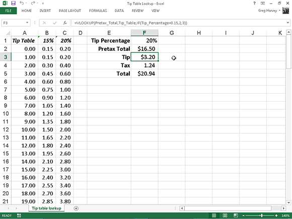
Figure 6-1: Using the VLOOKUP function to return the amount of the tip to add from a Lookup table.

To use this tip table, enter the percentage of the tip (15% or 20%) in cell F1 (named Tip_Percentage) and the amount of the check before tax in cell F2 (named Pretax_Total). Excel then looks up the value that you enter in the Pretax_Total cell in the first column of the Lookup table, which includes the cell range A2:C101 and is named Tip_Table.

Excel then moves down the values in the first column of Tip_Table until it finds a match, whereupon the program uses the col_index_num argument in the VLOOKUP function to determine which tip amount from that row of the table to return to cell F3. If Excel finds that the value entered in the Pretax_Total cell ($16.50 in this example) doesn’t exactly match one of the values in the first column of Tip_Table, the program continues to search down the comparison range until it encounters the first value that exceeds the pretax total (17.00 in cell A19 in this example). Excel then moves back up to the previous row in the table and returns the value in the column that matches the col_index_num argument of the VLOOKUP function. (This is because the optional range_lookup argument has been omitted from the function.)

Note that the tip table example in Figure 6-1 uses an IF function to determine the col_index_num argument for the VLOOKUP function in cell F3. The IF function determines the column number to be used in the tip table by matching the percentage entered in Tip_Percentage (cell F1) with 0.15. If they match, the function returns 2 as the col_index_num argument and the VLOOKUP function returns a value from the second column (the 15% column B) in the Tip_Table range. Otherwise, the IF function returns 3 as the col_index_num argument and the VLOOKUP function returns a value from the third column (the 20% column C) in the Tip_Table range.

Figure 6-2 shows an example that uses the HLOOKUP function to look up the price of each bakery item stored in a separate price Lookup table and then to return that price to the Price/Doz column of the Daily Sales list. Cell F3 contains the original formula with the HLOOKUP function that is then copied down column F:

=HLOOKUP(item,Price_table,2,FALSE)

In this HLOOKUP function, the range name Item that’s given to the Item column in the range C3:C62 is defined as the lookup_value argument and the cell range name Price table that’s given to the cell range I1:M2 is the table_array argument. The row_index_num argument is 2 because you want Excel to return the prices in the second row of the Prices Lookup table, and the optional range_lookup argument is FALSE because the item name in the Daily Sales list must match exactly the item name in the Prices Lookup table.

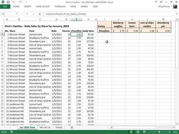
Figure 6-2: Using the HLOOKUP function to return the price of a bakery item from a Lookup table.

By having the HLOOKUP function use the Price table range to input the price per dozen for each bakery goods item in the Daily Sales list, you make it a very simple matter to update any of the sales in the list. All you have to do is change its Price/Doz cost in this range, and the HLOOKUP function immediately updates the new price in the Daily Sales list wherever the item is sold.

Performing a two-way lookup

In both the VLOOKUP and HLOOKUP examples, Excel only compares a single value in the data list to a single value in the vertical or horizontal Lookup table. Sometimes, however, you may have a table in which you need to perform a two-way lookup, whereby a piece of data is retrieved from the Lookup table based on looking up a value in the top row (with the table’s column headings) and a value in the first column (with the table’s row headings).

Figure 6-3 illustrates a situation in which you would use two values, the production date and the part number, to look up the expected production. In the 2013 Production Schedule table, the production dates for each part form the column headings in the first row of the table, and the part numbers form the row headings in its first column of the table.

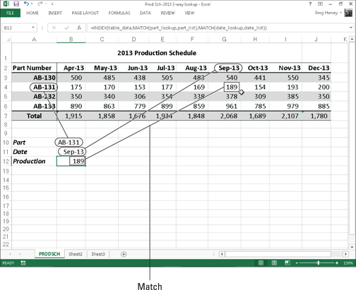
Figure 6-3: Doing a two-way lookup in the Production Schedule table.

To look up the number of the part scheduled to be produced in a particular month, you need to the use the MATCH function, which returns the relative position of a particular value in a cell range or array. The syntax of the MATCH function is as follows:

MATCH(lookup_value,lookup_array,[match_type])

The lookup_value argument is, of course, the value whose position you want returned when a match is found, and the lookup_array is the cell range or array containing the values that you want to match. The optional match_type argument is the number 1, 0, or –1, which specifies how Excel matches the value specified by the lookup_value argument in the range specified by the lookup_array argument:

Use match_type 1 to find the largest value that is less than or equal to the lookup_value. Note that the values in the lookup_array must be placed in ascending order when you use the 1 match_type argument. (Excel uses this type of matching when the match_type argument is omitted from the MATCH function.)

Use match_type 0 to find the first value that is exactly equal to the lookup_value. Note that the values in the lookup_array can be in any order when you use the 0 match_type argument.

Use match_type –1 to find the smallest value that is greater than or equal to the lookup_value. Note that the values in the lookup_array must be placed in descending order when you use the –1 match_type argument.

In addition to looking up the position of the production date and part number in the column and row headings in the Production Schedule table, you need to use an INDEX function, which uses the relative row and column number position to return the number to be produced from the table itself. The INDEX function follows two different syntax forms: array and reference. You use the array form when you want a value returned from the table (as you do in this example), and you use the reference form when you want a reference returned from the table.

The syntax of the array form of the INDEX function is as follows:

INDEX(array,[row_num],[col_num])

The syntax of the reference form of the INDEX function is as follows:

INDEX(reference,[row_num],[col_num],[area_num])

The array argument of the array form of the INDEX function is a range of cells or an array constant that you want Excel to use in the lookup. If this range or constant contains only one row or column, the corresponding row_num or col_num arguments are optional. If the range or array constant has more than one row or more than one column, and you specify both the row_num and the col_num arguments, Excel returns the value in the array argument that is located at the intersection of the row_num argument and the col_num argument.

For the MATCH and INDEX functions in the example shown in Figure 6-3, I assigned the following range names to the following cell ranges:

table_data to the cell range A2:J6 with the production data plus column and row headings

part_list to the cell range A2:A6 with the row headings in the first column of the table

date_list to the cell range A2:J2 with the column headings in the first row of the table

part_lookup to cell B10 that contains the name of the part to look up in the table

date_lookup to cell B11 that contains the name of the production date to look up in the table

As Figure 6-3 shows, cell B12 contains a rather long and — at first glance — complex formula using the range names outlined previously and combining the INDEX and MATCH functions:

=INDEX(table_data,MATCH(part_lookup,part_list),MATCH(date_lookup,date_list))

So you can better understand how this formula works, I break the formula down into its three major components: the first MATCH function that returns the row_num argument for the INDEX function, the second MATCH function that returns the col_num argument for the INDEX function, and the INDEX function itself that uses the values returned by the two MATCH functions to return the number of parts produced.

The first MATCH function that returns the row_num argument for the INDEX function is

MATCH(part_lookup,part_list)

This MATCH function uses the value input into cell B10 (named part_lookup) and looks up its position in the cell range A2:A6 (named part_list). It then returns this row number to the INDEX function as its row_num argument. In the case of the example shown in Figure 6-3 where part AB-131 is entered in the part_lookup cell in B10, Excel returns 3 as the row_num argument to the INDEX function.

The second MATCH function that returns the col_num argument for the INDEX function is

MATCH(date_lookup,date_list)

This second MATCH function uses the value input into cell B11 (named date_lookup) and looks up its position in the cell range A2:J2 (named date_list). It then returns this column number to the INDEX function as its col_num argument. In the case of the example shown in Figure 6-3 where September 1, 2010 (formatted as Sep-10), is entered in the date_lookup cell in B11, Excel returns 7 as the col_num argument to the INDEX function.

This means that for all its supposed complexity, the INDEX function shown on the Formula bar in Figure 6-3 contains the equivalent of the following formula:

=INDEX(table_data,3,7)

As Figure 6-3 shows, Excel returns 189 units as the planned production value for part AB-131 in September, 2013. You can verify that this is correct by manually counting the rows and the columns in the table_data range (cell range A2:J6). If you count down three rows (including row 2, the first row of this range), you come to Part 131 in column A. If you then count seven columns over (including column A with Part-131), you come to cell G4 in the Sep-13 column with the value 189.

Reference functions

The reference functions on the Lookup & Reference command button’s drop-down list on the Formulas tab of the Ribbon are designed to deal specifically with different aspects of cell references in the worksheet. This group of functions includes:

ADDRESS to return a cell reference as a text entry in a cell of the worksheet

AREAS to return the number of areas in a list of values (areas are defined as a range of contiguous cells or a single cell in the cell reference)

COLUMN to return the number representing the column position of a cell reference

COLUMNS to return the number of columns in a reference

FORMULATEXT to return the formula referenced as a text string

GETPIVOTDATA to return data stored in an Excel pivot table (see Book VII, Chapter 2 for details)

HYPERLINK to create a link that opens another document stored on your computer, network, or the Internet (you can also do this with the Insert⇒Hyperlink command — see Book IV, Chapter 2 for details)

INDIRECT to return a cell reference specified by a text string and bring the contents in the cell to which it refers to that cell

LOOKUP to return a value from an array

OFFSET to return a reference to a cell range that’s specified by the number of rows and columns from a cell or a cell range

ROW to return the row number of a cell reference

ROWS to return the number of rows in a cell range or array

RTD to return real-time data from a server running a program that supports COM (Component Object Model) automation

TRANSPOSE to return a vertical array as a horizontal array and vice versa

Get the skinny on columns and rows

The COLUMNS and ROWS functions return the number of columns and rows in a particular cell range or array. For example, if you have a cell range in the spreadsheet named product_mix, you can find out how many columns it contains by entering this formula:

=COLUMNS(product_mix)

If you want to know how many rows this range uses, you then enter this formula:

=ROWS(product_mix)

As indicated in the previous chapter, you can use the COLUMNS and ROWS functions together to calculate the total number of cells in a particular range. For example, if you want to know the exact number of cells used in the product_mix cell range, you create the following simple multiplication formula by using the COLUMNS and ROWS functions:

=COLUMNS(product_mix)*ROWS(product_mix)

Don’t confuse the COLUMNS (plural) function with the COLUMN (singular) function and the ROWS (plural) function with the ROW (singular) function. The COLUMN function returns the number of the column (as though Excel were using the R1C1 reference system) for the cell reference that you specify as its sole argument. Likewise, the ROW function returns the number of the row for the cell reference that you specify as its argument.

Transposing cell ranges

The TRANSPOSE function enables you to change the orientation of a cell range (or an array — see the section on entering array formulas in Book III, Chapter 1 for details). You can use this function to transpose a vertical cell range where the data runs down the rows of adjacent columns to one where the data runs across the columns of adjacent rows and vice versa. To successfully use the TRANSPOSE function, not only must you select a range that has an opposite number of columns and rows, but you must also enter it as an array formula.

For example, if you’re using the TRANSPOSE function to transpose a 2 x 5 cell range (that is, a range that takes up two adjacent rows and five adjacent columns), you must select a blank 5 x 2 cell range (that is, a range that takes five adjacent rows and two adjacent columns) in the worksheet before you use the Insert Function button to insert the TRANSPOSE function in the first cell. Then, after selecting the 2 x 5 cell range that contains the data that you want to transpose in the Array text box of the Function Arguments dialog box, you need to press Ctrl+Shift+Enter to close this dialog box and enter the TRANSPOSE function into the entire selected cell range as an array formula (enclosed in curly braces).

Suppose that you want to transpose the data entered into the cell range A10:C11 (a 2 x 3 array) to the blank cell range E10:F12 (a 3 x 2 array) of the worksheet. When you press Ctrl+Shift+Enter to complete the array formula, after selecting the cell range A10:C11 as the array argument, Excel puts the following array formula in every cell of the range:

{=TRANSPOSE(A10:C11)}

Figure 6-4 illustrates the use of the TRANSPOSE function. The cell range B2:C4 contains the original 3 x 2 array that I showed earlier in Figure 1-9 in Book III, Chapter 1 when discussing how you add array formulas to your worksheet. To convert this 3 x 2 array in the cell range B2:C4 to a 2 x 3 array in the range B6:D7, I followed these steps:

1. Select the blank cell range B6:D7 in the worksheet.

2. Click the Lookup & Reference command button on the Ribbon’s Formulas tab and then choose the TRANSPOSE option from the button’s drop-down menu.

Excel inserts =TRANSPOSE() on the Formula bar and opens the Function Arguments dialog box where the Array argument text box is selected.

3. Drag through the cell range B2:C4 in the worksheet so that the Array argument text box contains B2:C4 and the formula on the Formula bar now reads =TRANSPOSE(B2:C4).

4. Press Ctrl+Shift+Enter to close the Insert Arguments dialog box (don’t click OK) and to insert the TRANSPOSE array formula into the cell range B6:D7 as shown in Figure 6-4.

Clicking the OK button in the Function Arguments dialog box inserts the TRANSPOSE function into the active cell of the current cell selection. Doing this returns the #VALUE! error value to the cell. You must remember to press Ctrl+Shift+Enter to both close the dialog box and put the formula into the entire cell range.

If all you want to do is transpose row and column headings or a simple table of data, you don’t have to go through the rigmarole of creating an array formula using the TRANSPOSE function. Simply copy the range of cells to be transposed with the Copy command button on the Home tab of the Ribbon. Position the cell cursor in the first empty cell where the transposed range is to be pasted before you click the Transpose option on the Paste command button’s drop-down menu.

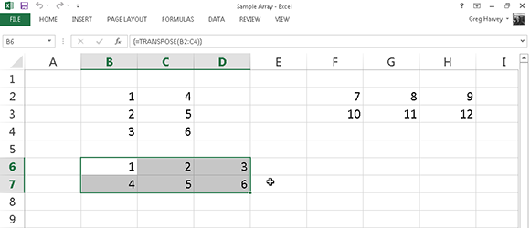
Figure 6-4: Using the TRANSPOSE function to change the orientation of a simple array.

Information, Please . . .

The information functions on the continuation menu accessed by clicking the More Functions command button on the Formulas tab of the Ribbon and then highlighting the Information option (or by pressing Alt+MQI) consist of a number of functions designed to test the contents of a cell or cell range and give you information on its current contents.

These kinds of information functions are often combined with IF functions, which determine what type of calculation, if any, to perform. The information function then becomes the logical_test argument of the IF function, and the outcome of the test, expressed as the logical TRUE or logical FALSE value, decides whether its value_if_true or its value_if_false argument is executed. (See Book III, Chapter 2 for information on using information functions that test for error values to trap errors in a spreadsheet.)

In addition to the many information functions that test whether the contents of a cell are of a certain type, Excel offers a smaller set of functions that return coded information about a cell’s contents or formatting and about the current operating environment in which the workbook is functioning. The program also offers an N (for Number) function that returns the value in a cell and an NA (for Not Available) function that inserts the #N/A error value in the cell.

Getting specific information about a cell

The CELL function is the basic information function for getting all sorts of data about the current contents and formatting of a cell. The syntax of the CELL function is

CELL(info_type,[reference])

The info_type argument is a text value that specifies the type of cell information you want returned. The optional reference argument is the reference of the cell range for which you want information. When you omit this argument, Excel specifies the type of information specified by the info_type argument for the last cell that was changed in the worksheet. When you specify a cell range as the reference argument, Excel returns the type of information specified by the info_type argument for the first cell in the range (that is, the one in the upper-left corner, which may or may not be the active cell of the range).

Table 6-1 shows the various info_type arguments that you can specify when using the CELL function. Remember that you must enclose each info_type argument in the CELL function in double-quotes (to enter them as text values) to prevent Excel from returning the #NAME? error value to the cell containing the CELL function formula. So, for example, if you want to return the contents of the first cell in the range B10:E80, you enter the following formula:

=CELL(“contents”,B10:E80)

Table 6-1 The CELL Functions info_type Arguments

CELL Function info_type Argument	Returns This Information
“address”	Cell address of the first cell in the reference as text using absolute cell references
“col”	Column number of the first cell in the reference
“color”	1 when the cell is formatted in color for negative values; otherwise returns 0 (zero)
“contents”	Value of the upper-left cell in the reference
“filename”	Filename (including the full pathname) of the file containing the cell reference: returns empty text (“”) when the workbook containing the reference has not yet been saved
“format”	Text value of the number format of the cell (see Table 6-2): Returns “-” at the end of the text value when the cell is formatted in color for negative values and “()” when the value is formatted with parentheses for positive values or for all values
“parentheses”	1 when the cell is formatted with parentheses for positive values or for all values
“prefix”	Text value of the label prefix used in the cell: Single quote (‘) when text is left-aligned; double quote (“) when text is right-aligned; caret (^) when text is centered; backslash () when text is fill-aligned; and empty text (“”) when the cell contains any other type of entry
“protect”	0 when the cell is unlocked and 1 when the cell is locked (see Book IV, Chapter 1 for details on protecting cells in a worksheet)
“row”	Row number of the first cell in the reference
“type”	Text value of the type of data in the cell: “b” for blank when cell is empty; “l” for label when cell contains text constant; and “v” for value when cell contains any other entry
“width”	Column width of the cell rounded off to the next highest integer (each unit of column width is equal to the width of one character in Excel’s default font size)

Table 6-2 shows the different text values along with their number formats (codes) that can be returned when you specify “format” as the info_type argument in a CELL function. (Refer to Book II, Chapter 3 for details on number formats and the meaning of the various number format codes.)

Table 6-2 Text Values Returned by the “format” info_type

Text Value	Number Formatting
“G”	General
“F0”	0
“,0”	#,##0
“F2”	0.00
“,2”	#,##0.00
“C0”	$#,##0_);($#,##0)
“C0-”	$#,##0_);[Red]($#,##0)
“C2”	$#,##0.00_);($#,##0.00)
“C2-”	$#,##0.00_);[Red]($#,##0.00)
“P0”	0%
“P2”	0.00%
“S2”	0.00E+00
“G”	# ?/? or # ??/??
“D4”	m/d/yy or m/d/yy h:mm or mm/dd/yy
“D1”	d-mmm-yy or dd-mmm-yy
“D2”	d-mmm or dd-mmm
“D3”	mmm-yy
“D5”	mm/dd
“D7”	h:mm AM/PM
“D6”	h:mm:ss AM/PM
“D9”	h:mm
“D8”	h:mm:ss

For example, if you use the CELL function that specifies “format” as the info_type argument on cell range A10:C28 (which you’ve formatted with the Comma style button on the Formula bar), as in the following formula

=CELL(“format”,A10:C28)

Excel returns the text value “,2-” (without the quotation marks) in the cell where you enter this formula signifying that the first cell uses the Comma style format with two decimal places and that negative values are displayed in color (red) and enclosed in parentheses.

Are you my type?

Excel provides another information function that returns the type of value in a cell. Aptly named, the TYPE function enables you to build formulas with the IF function that execute one type of behavior when the cell being tested contains a value and another when it contains text. The syntax of the TYPE function is

TYPE(value)

The value argument of the TYPE function can be any Excel entry: text, number, logical value, or even an Error value or a cell reference that contains such a value. The TYPE function returns the following values, indicating the type of contents:

1 for numbers

2 for text

4 for logical value (TRUE or FALSE)

16 for Error value

64 for an array range or constant (see Book III, Chapter 1)

The following formula combines the CELL and TYPE functions nested within an IF function. This formula returns the type of the number formatting used in cell D11 only when the cell contains a value. Otherwise, it assumes that D11 contains a text entry, and it evaluates the type of alignment assigned to the text in that cell:

=IF(TYPE(D11)=1,CELL(“format”,D11),CELL(“prefix”,D11))

Using the IS functions

The IS information functions (as in ISBLANK, ISERR, and so on) are a large group of functions that perform essentially the same task. They evaluate a value or cell reference and return the logical TRUE or FALSE, depending on whether the value is or isn’t the type for which the IS function tests. For example, if you use the ISBLANK function to test the contents of cell A1 as in

=ISBLANK(A1)

Excel returns TRUE to the cell containing the formula when A1 is empty and FALSE when it’s occupied by any type of entry.

Excel offers ten built-in IS information functions:

ISBLANK(value) to evaluate whether the value or cell reference is empty

ISERR(value) to evaluate whether the value or cell reference contains an Error value (except for #N/A)

ISERROR(value) to evaluate whether the value or cell reference contains an Error value (including #N/A)

ISLOGICAL(value) to evaluate whether the value or cell reference contains the logical TRUE or FALSE value

ISNA(value) to evaluate whether the value or cell reference contains the special #N/A Error value

ISNONTEXT(value) to evaluate whether the value or cell reference contains any type of entry other than text

ISNUMBER(value) to evaluate whether the value or cell reference contains a number

ISODD(number) to evaluate whether the value in the referenced cell is odd (TRUE) or even (FALSE)

ISREF(value) to evaluate whether the value or cell reference is itself a cell reference

ISTEXT(value) to evaluate whether the value or cell reference contains a text entry

In addition to these ten IS functions, Excel adds two more, ISEVEN and ISODD, when you activate the Analysis ToolPak add-in. The ISEVEN function evaluates whether the number or reference to a cell containing a number is even, whereas the ISODD function evaluates whether it is odd. (For an example of how to use the ISERROR function, refer to the section on error trapping in Book III, Chapter 2.)

Much Ado about Text

Normally, when you think of doing calculations in a spreadsheet, you think of performing operations on its numeric entries. You can, however, use the text functions as well as the concatenation operator (&) to perform operations on its text entries as well (referred to collectively as string operations).

Using text functions

Text functions found on the Text command button’s drop-down menu on the Ribbon’s Formulas tab (Alt+MT) include two types of functions: functions such as VALUE, TEXT, and DOLLAR that convert numeric text entries into numbers and numeric entries into text, and functions such as UPPER, LOWER, and PROPER that manipulate the strings of text themselves.

Many times, you need to use the text functions when you work with data from other programs. For example, suppose that you purchase a target client list on disk, only to discover that all the information has been entered in all uppercase letters. In order to use this data with your word processor’s mail merge feature, you would use Excel’s PROPER function to convert the entries so that only the initial letter of each word is in uppercase.

Text functions such as the UPPER, LOWER, and PROPER functions all take a single text argument that indicates the text that should be manipulated. The UPPER function converts all letters in the text argument to uppercase. The LOWER function converts all letters in the text argument to lowercase. The PROPER function capitalizes the first letter of each word as well as any other letters in the text argument that don’t follow another letter, and changes all other letters in the text argument to lowercase.

Figure 6-5 illustrates a situation in which you would use the PROPER function. Here, both last and first name text entries have been made in all uppercase letters. Follow these steps for using the PROPER function to convert text entries to the proper capitalization:

1. Position the cell cursor in cell C3 and then click the Text command button on the Ribbon’s Formulas tab (or press Alt+MT) and then choose PROPER from its drop-down menu.

The Function Arguments dialog box for the PROPER function opens with the Text box selected.

2. Click cell A3 in the worksheet to insert A3 in the Text box of the Function Arguments dialog box and then click OK to insert the PROPER function into cell C3.

Excel closes the Insert Function dialog box and inserts the formula =PROPER(A3) in cell C3, which now contains the proper capitalization of the last name Aiken.

3. Drag the Fill handle in the lower-right corner of cell C3 to the right to cell D3 and then release the mouse button to copy the formula with the PROPER function to this cell.

Excel now copies the formula =PROPER(B3) to cell D3, which now contains the proper capitalization of the first name, Christopher. Now you’re ready to copy these formulas with the PROPER function down to row 17.

4. Drag the fill handle in the lower-right corner of cell D3 down to cell D17 and then release the mouse button to copy the formulas with the PROPER function down.

The cell range C3:D17 now contains first and last name text entries with the proper capitalization. (See Figure 6-5.) Before replacing all the uppercase entries in A3:B17 with these proper entries, you convert them to their calculated values. This action replaces the formulas with the text as though you had typed each name in the worksheet.

5. With the cell range C3:D17 still selected, click the Copy command button on the Home tab of the Ribbon.

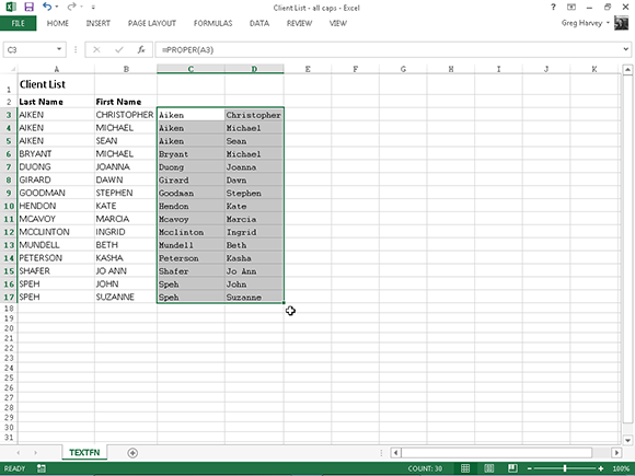
Figure 6-5: Using the PROPER function to convert names in all uppercase letters to proper capitalization.

6. Immediately choose the Paste Values option from the Paste command button’s drop-down menu.

You’ve now replaced the formulas with the appropriate text. Now you’re ready to move this range on top of the original range with the all-uppercase entries. This action will replace the uppercase entries with the ones using the proper capitalization.

7. With the cell range C3:D17 still selected, position the white-cross mouse or Touch pointer on the bottom of the range; when the pointer changes to an arrowhead, drag the cell range until its outline encloses the range A3:B17 and then release the mouse button or remove your finger or stylus from the touchscreen.

Excel displays an alert box asking if you want the program to replace the contents of the destination’s cells.

8. Click OK in the Alert dialog box to replace the all-uppercase entries with the properly capitalized ones in the destination cells.

Your worksheet now looks like the one shown in Figure 6-6. Everything is fine in the worksheet with the exception of the two last names, Mcavoy and Mcclinton. You have to manually edit cells A11 and A12 to capitalize the A in McAvoy and the second C in McClinton.

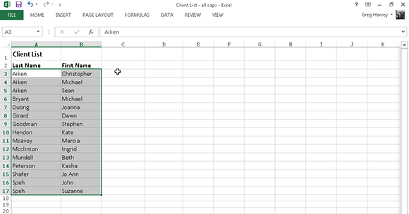
Figure 6-6: Worksheet after replacing names in all uppercase letters with properly capitalized names.

Concatenating text

You can use the ampersand (&) operator to concatenate (or join) separate text strings together. For example, in the Client list spreadsheet shown in Figure 6-6, you can use this operator to join together the first and last names currently entered in two side-by-side cells into a single entry, as shown in Figure 6-7.

To join the first name entry in cell B3 with the last name entry in cell A3, I entered the following formula in cell C3:

=B3&” “&A3

Notice the use of the double quotes in this formula. They enclose a blank space that is placed between the first and last names joined to them with the two concatenation operators. If I didn’t include this space in the formula and just joined the first and last names together with this formula

=B3&A3

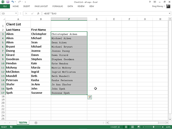
Figure 6-7: Spreadsheet after concatenating the first and last names in column C.

Excel would return ChristopherAiken to cell C3, all as one word.

After entering the concatenation formula that joins the first and last names in cell C3 separated by a single space, I then drag the Fill handle in cell C3 down to C17 to join all the other client names in a single cell in column C.

After the original concatenation formula is copied down the rows of column C, I copy the selected cell range C3:C17 to the Clipboard by clicking the Copy button in the Clipboard group of the Home tab on the Ribbon, and then I immediately choose the Paste Values option from the Paste command button’s drop-down menu. This action pastes calculated text values over the concatenation formulas, thereby replacing the original formulas. The result is a list of first and last names together in the same cell in the range C3:C17, as though I had manually input each one.