
11
Radio Planning
In Part III, we take a look at a big picture of wireless communication systems and use a top down approach. Many different interests are entangled in the wireless communications system design. The designed wireless communication system should satisfy various interested parties such as vendors, mobile operators, regulators, and mobile users. An officer of a regulatory agency takes a look at the wireless communication system in terms of an efficient spectrum usage and violation of the regulation for specific frequency bands. A mobile operator is interested in business opportunities, service quality, and the cost of the infrastructure. A mobile phone vendor or a network equipment vendor looks into the cost effective design of the wireless communication system. An end user is interested in good service quality and stylish mobile phones. For example, the designed wireless communication system copes with many channel impairments. The transmit power should be enough to cover users located in a cell edge. The battery life of a mobile phone should be long enough. It should support enough data rates at any place. The packet loss rate should be acceptable at any place. An end user is interested in whether or not it can use a network with enough data rates and seamless connection. Thus, we should consider all conditions and satisfy their requirements. In order to build wireless communication systems, we consider many system requirements such as spectrum, system capacity, service area, radio resource allocation, cost, and QoS. It is not easy to find an optimal solution for them but we should find a good trade-off. In Part III, we mainly deal with wireless communication network planning and wireless communication system integration. In this chapter, we focus on radio planning and link budget analysis.
11.1 Radio Planning and Link Budget Analysis
Since we have a limited radio resource, radio planning is an essential part of a wireless network design. The radio planning process deals with spectrum allocation, power assignment, base station location, configuration of a wireless communication system, and so on. The goal of radio planning is to provide sufficient coverage, capacity, and service quality. Basically, the radio planning process is composed of three steps: dimensioning, detailed planning, and optimization. The process of radio planning is iteratively carried out. The first step is dimensioning. It provides the initial estimation of the number and placement of base stations to meet the network requirements. We firstly collect the required system coverage, capacity, and service quality and then take into consideration population, geographical area (dense urban area, urban area, and rural area), frequency, propagation model, and so on. Thus, we perform link budget analysis, traffic analysis, coverage estimation, and capacity evaluation. We initially decide how many base stations are needed, where to deploy them, and how to configure base station parameters such as antenna type, transmit power, height, and frequency allocation. Based on the results of the dimensioning step, the detailed planning step obtains further detailed information such as site selection and acquisition, coverage calculation, capacity planning, and base station configuration. In this step, many software tools are employed to predict coverage, capacity, interference, and so on. A wireless network designer creates databases including geographical and statistical information and decides base station location and configuration in detail. In the optimization step, we use measurements from the wireless networks and adjust the settings of the base stations to achieve a better coverage and capacity. Basically, the radio and network planning is very complex and there is no optimal solution. The only way we can do is to find a better setting iteratively. Figure 11.1 illustrates the summary of the radio and network planning process.
Figure 11.1 Radio and network planning process
The dimensioning step starts from the link budget calculation. It can be defined as the signal strength gain and loss calculation on the path from a transmitter to a receiver. The purpose of the link budget calculation is to estimate the Maximum Allowable Path Loss (MAPL). It determines the cell size along with the geographical area and area coverage probability. It estimates the required numbers of bases stations. The MAPL is calculated as follows:
where the Equivalent Isotropic Radiated Power (EIRP) is the RF power that would be emitted by a theoretical isotropic antenna and P Rx is the received power. The EIRP considers all gains and losses in the transmitter and produces the peak power density observed in the direction of maximum antenna gain. It is represented as follows:
where P Tx, G Tx, and L Tx are the transmit power, the antenna gain, and the transmitter losses, respectively. The transmit power is determined by each regulation [1–4]. Tables 11.1 and 11.2 show the maximum transmit power levels for different Mobile Station (MS) (or User Equipment (UE)) classes in GSM and WCDMA.
Table 11.1 Maximum transmit powers for each MS class in GSM [1]
| MS classes | MS output power (dBm) |
| Class 1 | 43 |
| Class 2 | 39 |
| Class 3 | 37 |
| Class 4 | 33 |
Table 11.2 Maximum transmit powers for each UE class in WCDMA [2]
| UE classes | UE output power (dBm) |
| Class 1 | 33 |
| Class 2 | 27 |
| Class 3 | 24 |
| Class 4 | 21 |
Depending on MS (or UE) scenario, the maximum transmit powers are classified because it should not interfere with other MSs (or UEs). For LTE system, Tables 11.3 and 11.4 show the maximum transmit powers for UE and Base Station (BS), respectively.
Table 11.3 Maximum transmit powers for each UE class in LTE [3]
| CPE band | Class 2 (dBm) | Class 3 (dBm) |
| CPE_13 | 27 | 23 |
Table 11.4 Base station rated output power in LTE [4]
| BS class | Rated output power (PRAT) |
| Wide area BS | There is no upper limit for the rated output power of the Wide Area Base Station |
| Medium range BS | ≤ +38 dBm |
| Local area BS | ≤ +24 dBm |
| Home BS | ≤ +20 dBm (for one transmit antenna port) |
| ≤ +17 dBm (for two transmit antenna ports) | |
| ≤ +14 dBm (for four transmit antenna ports) | |
| < +11 dBm (for eight transmit antenna ports) |
In Table 11.3, the power class 2 and 3 are considered for indoor deployment and both indoor and outdoor deployment, respectively. The regulation basically allows about ±2 dBm tolerance of the maximum transmit power from each value. The antenna gain G Tx is expressed in decibels-isotropic (dBi). Since the antenna is a passive device, it does not amplify a signal. However, a base station does not use omnidirectional antennas but directional (sectiorized) antennas. Thus, it can produce a relative gain due to directivity. Antenna gain is defined as the ratio of the power produced by the antenna in a given direction to the power produced by a loss free isotropic antenna at the same field strength and distance. Figure 11.2 illustrates antenna gain definition. It can be simply expressed as follows:

where ε is the efficiency of antenna.

Figure 11.2 Antenna gain
There are several transmitter losses L Tx. The cable and connector loss is one of the main transmission losses. The value depends on the length, material, temperature, frequency, and so on. The cable manufacturer basically provides the attenuation value. The cable and connector loss of MS is zero because it does not use an external antenna. Instead, MS should take into account a body loss because a handset is close to a user’s head. Basically, a human head absorbs transmission energy and change polarization. The value of the body loss is about 3–5 dB. If a mobile user is located in a car or a building, an extra loss (car and building penetration loss) should be considered [5]. The received power is represented as follows:
where S Rx, G Rx, and L Rx are the receiver sensitivity, the receiver antenna gain, and receiver losses, respectively. The receiver sensitivity is the minimum received signal power which can successfully demodulate and decode the received signals. It is always expressed as a negative value and the typical value is in the range of −70 to −110 dBm. It is independent of a transmitter and depends on the receiver noise figure and the received signal-to-interference-plus-noise ratio (SINR). It can be represented as follows:
where SINR, N T, F Rx, and M i are the SINR, the thermal noise power per subcarrier, the receiver noise figure, and the implementation margin, respectively. The SINR can be defined as follows:
The required SINR is defined as the power ratio of the desired signal to total interferences and noise. The required SINR is one of the key parameters in wireless communication systems. It depends on modulation and coding schemes and channel models. Basically, a higher required SINR is needed when a high-order modulation and a low coding rate are used. The thermal noise N T is calculated as follows:
where k, T, and B are Boltzmann constant (1.38 × 10⁻²³ J/K), the temperature (K), and the bandwidth, respectively. The receiver noise figure is defined as follows:

where SNRin and SNRout are the input SNR and the output SNR in a RF device, respectively. It means how much thermal noises are added to the received signal in a RF device. Basically, it is expressed in decibels. (11.8) can be rewritten as follows:
If the receiver is composed of multiple cascaded RF devices, the total noise figure can be represented with Friis’s formula as follows:
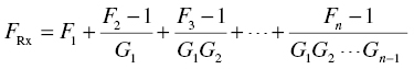
where Fi and Gi are the noise figure and the power gain of the ith device, respectively. The power gain is given by the manufacturer if it is an active device. However, if it is a passive device, there is an inverse relationship between the power gain and the transmission loss.
Basically, a shadowing and multipath fading effect occurs in wireless channels. Thus, a wireless communication and network designer should keep sufficient system gain to accommodate the fading effect for maintaining good service quality. Higher the fading margin M F provides the more reliable link quality. It depends on carrier frequency, distance between MS and BS, required reliability, and so on. As a rule of thumb, we need to have at least 15 dB as a fading margin.
In cellular systems, the interferences from own cells and neighboring cells always occur. A wireless communication and network designer should allow a network to secure an interference margin. This margin is related to cell load and coverage. Generally, a smaller interference margin is needed for coverage limited scenarios and a larger interference margin is needed for capacity limited scenarios. As cell load increases, addition interferences are generated from own cell and neighboring cells and the coverage shrinks. Namely, a larger interference margin is suggested when more loading is allowed in the network and smaller coverage is caused. The interference margin depends on cell load and G-factor. It can be defined as follows:
The typical values of the interference margin are 1–3 dB and the corresponding cell loading is 20–50% [6]. Figure 11.3 illustrates signal strength change from a transmitter to a receiver.

Figure 11.3 General link budget in wireless communication system
We now obtained the MAPL and can calculate the cell radius using a propagation model such as the free space model, the ray tracing model, and the empirical model. The empirical model is widely used in the network planning phase. For example, we have Hata’s formula [7] for an urban area as follows:
where f c is the carrier frequency (MHz), h bs is the base station antenna height (m), R is the cell radius (km), h ms is the mobile station antenna height (m), and a(h ms) is the correction factor for the effective mobile station antenna height. From (11.12), the cell radius is calculated as follows:
For a small size cell,
and for a large cell,

This cell radius means the signal beyond this radius is not reliable. Each cell has different correction factor and a propagation model is adopted according to the type of surroundings (urban, suburban, and rural) and cell deployments (macrocell, microcell, and femtocell). Thus, the MAPL and cell radius should be separately calculated for each area. Once the cell radius is decided, the cell area A cell is calculated as follows:
where α is 2.6 (omnidirectional site), 1.3 (2 sector site), and 1.95 (3 sector site) in the hexagonal cell model [8]. Figure 11.4 illustrates different types of sites.

Figure 11.4 Omnidirectional site (a), 2 sector site (b), and 3 sector site (c)

Figure 11.5 Link budget of Example 11.1
Based on the link budget analysis, we estimated the coverage which guarantees the signal reliability. Now, we take a look into capacity planning. It provides us with demanded resources and available traffics and estimates subscribers supported per a site. In order to calculate the capacity, we need to define several terms such as busy hour, overbooking factor, and interference. The busy hour is the traffic engineering measurement representing the greatest traffic and call attempts in a day. As a rule of thumb, the busy hour average loading is 50% and it carries 15% daily traffic. The overbooking factor is based on the fact that only small number of subscribers uses a radio resource simultaneously. For example, if a user data rate is 1 Mbps and an average data rate per a subscriber during a busy hour is 20 kbps, the overbooking factor is 50 (=1 Mbps/20 kbps). Once system requirements are given, we can calculate the number of subscribers per site. In order to meet the target user data rate, the number of subscribers per site is calculated as shown in Table 11.5.
Table 11.5 Subscribers per site calculation based on data rate
| System parameters | Variables |
| Bandwidth | a (Hz) |
| Spectral efficiency | b (bps/Hz) |
| Cell average capacity | c = ab (bps) |
| Busy hour average loading | d (%) |
| Required user data rate | e (bps/subscriber) |
| Overbooking factor | f |
| Average busy hour data rate per subscriber | g = e/f (bps) |
| The number of sectors per site | h |
| Subscribers per site | cdh/g (subscriber/site) |
In order to meet the traffic requirements and find suitable network configurations, the subscribers per site should be calculated in terms of traffic demands. The number of subscribers per site is calculated as shown in Table 11.6.
Table 11.6 Subscribers per site calculation based on traffic
| System parameters | Variables |
| Bandwidth | a (Hz) |
| Spectral efficiency | b (Mbps/Hz) |
| Cell average capacity | c = ab (Mbps) |
| Required traffic | d = c × (3600/8192) (GB/h) |
| Busy hour average loading | e (%) |
| Busy hour carries of daily traffic | f (%) |
| Convert to month | 30 |
| The number of sectors per site | g |
| The required user traffic | h |
| Subscribers per site | 30deg/fh (subscriber/site/month) |
Table 11.7 Subscribers per site calculation based on user data rate
| System parameters | Variable |
| Bandwidth | 20 MHz |
| Spectral efficiency | 1.5 bps/Hz |
| Cell average capacity | 30 Mbps = 20 MHz × 1.5 bps/Hz |
| Busy hour average loading | 50% |
| Required user data rate | 1 Mbps/subscriber |
| Overbooking factor | 20 |
| Average busy hour data rate per subscriber | 50 kbps = 1 Mbps/subscriber/20 |
| The number of sectors per site | 3 |
| Subscribers per site | 900 subscriber/site = 30 Mbps × 50% × 3/50 kbps |
Table 11.8 Subscribers per site calculation based on user traffic
| System parameters | Variable |
| Bandwidth | 20 Hz |
| Spectral efficiency | 1.5 Mbps/Hz |
| Cell average capacity | 30 Mbps |
| Required traffic | 13.18 GB/h |
| Busy hour average loading | 50% |
| Busy hour carries of daily traffic | 15% |
| Convert to month | 30 |
| The number of sectors per site | 3 |
| Subscribers per site | 989 subscriber/site/month = (30 × 13.18 GB/h × 0.5 × 3)/(0.15 × 4) |
11.2 Traffic Engineering
A customer visiting a bank wants to avoid a long queue. A car on a road does not want to be stuck in a traffic jam. Likewise, a mobile user does not want to wait a phone connection for a long time and expects a high quality service all the time. Thus, a wireless communication and network designer should manage a radio resource and provide a mobile user with adequate services. Traffic engineering deals with this issue. It is statistical techniques to predict the behavior of users and share network resources.
A Danish mathematician, A. K. Erlang, developed the fundamentals of trunking theory [9]. Many traffic models are based on his theory. Before discussing Erlang theory, we need to define several terms. Trunking is a concept in which many users share a limited radio resource. It allows n users to share the relatively small number of channels in a cell. The traffic unit, Erlang, means channel occupation ratio. For example, 0.5 Erlang means 30 min call for 1 h. The traffic intensity is a measure of the average channel occupancy during a specific time. It is measured in Erlang and denoted by A. The traffic intensity for one user is defined as follows:
where λ and H are the average number of channel/call request per unit time and the average occupancy duration of a channel/call, respectively. The total traffic intensity A is
The Grade of Service (GOS) is a measure of congestion, which is specified as the probability that a call is blocked or that a call is delayed. A blocked/lost call means inability to allocate a channel/call due to congestion. Erlang B is a measure of the GOS and simply defines the call blocking probability. It is formulated as follows:

where N is the number of resources (or the trunked channels). The Erlang B model has the following assumptions:
- There is no set-up time when a service is requested.
- The requesting users are blocked when there is no available channel and try again later.
- It offers no queuing for call requests.
- The arrival of calls is determined by the Poisson process.
- We have an infinite number of users.
- All users may request a channel resource at any time.
- The holding time is exponentially distributed.
- A finite number of channels are available in the trunking pool.
Table 11.9 Erlang B Table
| No. of resources (N) | Traffic intensity in Erlangs (A) for Pb(N, A) | ||||||||||||||||
| 0.1% | 0.2% | 0.5% | 1% | 1.2% | 1.3% | 1.5% | 2% | 3% | 5% | 7% | 10% | 15% | 20% | 30% | 40% | 50% | |
| 1 | 0.001 | 0.002 | 0.005 | 0.010 | 0.012 | 0.013 | 0.02 | 0.020 | 0.031 | 0.053 | 0.075 | 0.111 | 0.176 | 0.250 | 0.429 | 0.667 | 1.00 |
| 2 | 0.046 | 0.065 | 0.105 | 0.153 | 0.168 | 0.176 | 0.19 | 0.223 | 0.282 | 0.381 | 0.470 | 0.595 | 0.796 | 1.00 | 1.45 | 2.00 | 2.73 |
| 3 | 0.194 | 0.249 | 0.349 | 0.455 | 0.489 | 0.505 | 0.53 | 0.602 | 0.715 | 0.899 | 1.06 | 1.27 | 1.60 | 1.93 | 2.63 | 3.48 | 4.59 |
| 4 | 0.439 | 0.535 | 0.701 | 0.869 | 0.922 | 0.946 | 0.99 | 1.09 | 1.26 | 1.52 | 1.75 | 2.05 | 2.50 | 2.95 | 3.89 | 5.02 | 6.50 |
| 5 | 0.762 | 0.900 | 1.13 | 1.36 | 1.43 | 1.46 | 1.52 | 1.66 | 1.88 | 2.22 | 2.50 | 2.88 | 3.45 | 4.01 | 5.19 | 6.60 | 8.44 |
| 6 | 1.15 | 1.33 | 1.62 | 1.91 | 2.00 | 2.04 | 2.11 | 2.28 | 2.54 | 2.96 | 3.30 | 3.76 | 4.44 | 5.11 | 6.51 | 8.19 | 10.4 |
| 7 | 1.58 | 1.80 | 2.16 | 2.50 | 2.60 | 2.65 | 2.73 | 2.94 | 3.25 | 3.74 | 4.14 | 4.67 | 5.46 | 6.23 | 7.86 | 9.80 | 12.4 |
| 8 | 2.05 | 2.31 | 2.73 | 3.13 | 3.25 | 3.30 | 3.40 | 3.63 | 3.99 | 4.54 | 5.00 | 5.60 | 6.50 | 7.37 | 9.21 | 11.4 | 14.3 |
| 9 | 2.56 | 2.85 | 3.33 | 3.78 | 3.92 | 3.98 | 4.08 | 4.34 | 4.75 | 5.37 | 5.88 | 6.55 | 7.55 | 8.52 | 10.6 | 13.0 | 16.3 |
| 10 | 3.09 | 3.43 | 3.96 | 4.46 | 4.61 | 4.68 | 4.80 | 5.08 | 5.53 | 6.22 | 6.78 | 7.51 | 8.62 | 9.68 | 12.0 | 14.7 | 18.3 |
| 11 | 3.65 | 4.02 | 4.61 | 5.16 | 5.32 | 5.40 | 5.53 | 5.84 | 6.33 | 7.08 | 7.69 | 8.49 | 9.69 | 10.9 | 13.3 | 16.3 | 20.3 |
| 12 | 4.23 | 4.64 | 5.28 | 5.88 | 6.05 | 6.14 | 6.27 | 6.61 | 7.14 | 7.95 | 8.61 | 9.47 | 10.8 | 12.0 | 14.7 | 18.0 | 22.2 |
| 13 | 4.83 | 5.27 | 5.96 | 6.61 | 6.80 | 6.89 | 7.03 | 7.40 | 7.97 | 8.83 | 9.54 | 10.5 | 11.9 | 13.2 | 16.1 | 19.6 | 24.2 |
| 14 | 5.45 | 5.92 | 6.66 | 7.35 | 7.56 | 7.65 | 7.81 | 8.20 | 8.80 | 9.73 | 10.5 | 11.5 | 13.0 | 14.4 | 17.5 | 21.2 | 26.2 |
| 15 | 6.08 | 6.58 | 7.38 | 8.11 | 8.33 | 8.43 | 8.59 | 9.01 | 9.65 | 10.6 | 11.4 | 12.5 | 14.1 | 15.6 | 18.9 | 22.9 | 28.2 |
| 16 | 6.72 | 7.26 | 8.10 | 8.88 | 9.11 | 9.21 | 9.39 | 9.83 | 10.5 | 11.5 | 12.4 | 13.5 | 15.2 | 16.8 | 20.3 | 24.5 | 30.2 |
| 17 | 7.38 | 7.95 | 8.83 | 9.65 | 9.89 | 10.0 | 10.19 | 10.7 | 11.4 | 12.5 | 13.4 | 14.5 | 16.3 | 18.0 | 21.7 | 26.2 | 32.2 |
| 18 | 8.05 | 8.64 | 9.58 | 10.4 | 10.7 | 10.8 | 11.00 | 11.5 | 12.2 | 13.4 | 14.3 | 15.5 | 17.4 | 19.2 | 23.1 | 27.8 | 34.2 |
| 19 | 8.72 | 9.35 | 10.3 | 11.2 | 11.5 | 11.6 | 11.82 | 12.3 | 13.1 | 14.3 | 15.3 | 16.6 | 18.5 | 20.4 | 24.5 | 29.5 | 36.2 |
| 20 | 9.41 | 10.1 | 11.1 | 12.0 | 12.3 | 12.4 | 12.65 | 13.2 | 14.0 | 15.2 | 16.3 | 17.6 | 19.6 | 21.6 | 25.9 | 31.2 | 38.2 |
| 21 | 10.1 | 10.8 | 11.9 | 12.8 | 13.1 | 13.3 | 13.48 | 14.0 | 14.9 | 16.2 | 17.3 | 18.7 | 20.8 | 22.8 | 27.3 | 32.8 | 40.2 |
| 22 | 10.8 | 11.5 | 12.6 | 13.7 | 14.0 | 14.1 | 14.32 | 14.9 | 15.8 | 17.1 | 18.2 | 19.7 | 21.9 | 24.1 | 28.7 | 34.5 | 42.1 |
| 23 | 11.5 | 12.3 | 13.4 | 14.5 | 14.8 | 14.9 | 15.16 | 15.8 | 16.7 | 18.1 | 19.2 | 20.7 | 23.0 | 25.3 | 30.1 | 36.1 | 44.1 |
| 24 | 12.2 | 13.0 | 14.2 | 15.3 | 15.6 | 15.8 | 16.01 | 16.6 | 17.6 | 19.0 | 20.2 | 21.8 | 24.2 | 26.5 | 31.6 | 37.8 | 46.1 |
| 25 | 13.0 | 13.8 | 15.0 | 16.1 | 16.5 | 16.6 | 16.87 | 17.5 | 18.5 | 20.0 | 21.2 | 22.8 | 25.3 | 27.7 | 33.0 | 39.4 | 48.1 |
| 26 | 13.7 | 14.5 | 15.8 | 17.0 | 17.3 | 17.5 | 17.72 | 18.4 | 19.4 | 20.9 | 22.2 | 23.9 | 26.4 | 28.9 | 34.4 | 41.1 | 50.1 |
| 27 | 14.4 | 15.3 | 16.6 | 17.8 | 18.2 | 18.3 | 18.59 | 19.3 | 20.3 | 21.9 | 23.2 | 24.9 | 27.6 | 30.2 | 35.8 | 42.8 | 52.1 |
| 28 | 15.2 | 16.1 | 17.4 | 18.6 | 19.0 | 19.2 | 19.45 | 20.2 | 21.2 | 22.9 | 24.2 | 26.0 | 28.7 | 31.4 | 37.2 | 44.4 | 54.1 |
| 29 | 15.9 | 16.8 | 18.2 | 19.5 | 19.9 | 20.0 | 20.32 | 21.0 | 22.1 | 23.8 | 25.2 | 27.1 | 29.9 | 32.6 | 38.6 | 46.1 | 56.1 |
| 30 | 16.7 | 17.6 | 19.0 | 20.3 | 20.7 | 20.9 | 21.19 | 21.9 | 23.1 | 24.8 | 26.2 | 28.1 | 31.0 | 33.8 | 40.0 | 47.7 | 58.1 |
| 31 | 17.4 | 18.4 | 19.9 | 21.2 | 21.6 | 21.8 | 22.07 | 22.8 | 24.0 | 25.8 | 27.2 | 29.2 | 32.1 | 35.1 | 41.5 | 49.4 | 60.1 |
| 32 | 18.2 | 19.2 | 20.7 | 22.0 | 22.5 | 22.6 | 22.95 | 23.7 | 24.9 | 26.7 | 28.2 | 30.2 | 33.3 | 36.3 | 42.9 | 51.1 | 62.1 |
| 33 | 19.0 | 20.0 | 21.5 | 22.9 | 23.3 | 23.5 | 23.83 | 24.6 | 25.8 | 27.7 | 29.3 | 31.3 | 34.4 | 37.5 | 44.3 | 52.7 | 64.1 |
| 34 | 19.7 | 20.8 | 22.3 | 23.8 | 24.2 | 24.4 | 24.72 | 25.5 | 26.8 | 28.7 | 30.3 | 32.4 | 35.6 | 38.8 | 45.7 | 54.4 | 66.1 |
| 35 | 20.5 | 21.6 | 23.2 | 24.6 | 25.1 | 25.3 | 25.60 | 26.4 | 27.7 | 29.7 | 31.3 | 33.4 | 36.7 | 40.0 | 47.1 | 56.0 | 68.1 |
| 36 | 21.3 | 22.4 | 24.0 | 25.5 | 26.0 | 26.2 | 26.49 | 27.3 | 28.6 | 30.7 | 32.3 | 34.5 | 37.9 | 41.2 | 48.6 | 57.7 | 70.1 |
| 37 | 22.1 | 23.2 | 24.8 | 26.4 | 26.8 | 27.0 | 27.39 | 28.3 | 29.6 | 31.6 | 33.3 | 35.6 | 39.0 | 42.4 | 50.0 | 59.4 | 72.1 |
| 38 | 22.9 | 24.0 | 25.7 | 27.3 | 27.7 | 27.9 | 28.28 | 29.2 | 30.5 | 32.6 | 34.4 | 36.6 | 40.2 | 43.7 | 51.4 | 61.0 | 74.1 |
| 39 | 23.7 | 24.8 | 26.5 | 28.1 | 28.6 | 28.8 | 29.18 | 30.1 | 31.5 | 33.6 | 35.4 | 37.7 | 41.3 | 44.9 | 52.8 | 62.7 | 76.1 |
| 40 | 24.4 | 25.6 | 27.4 | 29.0 | 29.5 | 29.7 | 30.08 | 31.0 | 32.4 | 34.6 | 36.4 | 38.8 | 42.5 | 46.1 | 54.2 | 64.4 | 78.1 |
| 41 | 25.2 | 26.4 | 28.2 | 29.9 | 30.4 | 30.6 | 30.98 | 31.9 | 33.4 | 35.6 | 37.4 | 39.9 | 43.6 | 47.4 | 55.7 | 66.0 | 80.1 |
| 42 | 26.0 | 27.2 | 29.1 | 30.8 | 31.3 | 31.5 | 31.88 | 32.8 | 34.3 | 36.6 | 38.4 | 40.9 | 44.8 | 48.6 | 57.1 | 67.7 | 82.1 |
| 43 | 26.8 | 28.1 | 29.9 | 31.7 | 32.2 | 32.4 | 32.79 | 33.8 | 35.3 | 37.6 | 39.5 | 42.0 | 45.9 | 49.9 | 58.5 | 69.3 | 84.1 |
| 44 | 27.6 | 28.9 | 30.8 | 32.5 | 33.1 | 33.3 | 33.69 | 34.7 | 36.2 | 38.6 | 40.5 | 43.1 | 47.1 | 51.1 | 59.9 | 71.0 | 86.1 |
| 45 | 28.4 | 29.7 | 31.7 | 33.4 | 34.0 | 34.2 | 34.60 | 35.6 | 37.2 | 39.6 | 41.5 | 44.2 | 48.2 | 52.3 | 61.3 | 72.7 | 88.1 |
| 46 | 29.3 | 30.5 | 32.5 | 34.3 | 34.9 | 35.1 | 35.51 | 36.5 | 38.1 | 40.5 | 42.6 | 45.2 | 49.4 | 53.6 | 62.8 | 74.3 | 90.1 |
| 47 | 30.1 | 31.4 | 33.4 | 35.2 | 35.8 | 36.0 | 36.42 | 37.5 | 39.1 | 41.5 | 43.6 | 46.3 | 50.6 | 54.8 | 64.2 | 76.0 | 92.1 |
| 48 | 30.9 | 32.2 | 34.2 | 36.1 | 36.7 | 36.9 | 37.34 | 38.4 | 40.0 | 42.5 | 44.6 | 47.4 | 51.7 | 56.0 | 65.6 | 77.7 | 94.1 |
| 49 | 31.7 | 33.0 | 35.1 | 37.0 | 37.6 | 37.8 | 38.25 | 39.3 | 41.0 | 43.5 | 45.7 | 48.5 | 52.9 | 57.3 | 67.0 | 79.3 | 96.1 |
| 50 | 32.5 | 33.9 | 36.0 | 37.9 | 38.5 | 38.7 | 39.17 | 40.3 | 41.9 | 44.5 | 46.7 | 49.6 | 54.0 | 58.5 | 68.5 | 81.0 | 98.1 |
The Erlang B model assumes the blocked requests are lost. However, Erlang C model describes the probability that a service requester will have to wait for a resource. If all servers are busy, the request is queued. Like the Erlang B, the Erlang C model is formulated as follows:

The probability P c(N, A) means that a service requester has to wait for service. The average delay is given by
where H is an average call holding time. The average number of requests in the queue is given by
The probability of the delay exceeding time t is given by
The Erlang B model has the following assumptions:
- An unlimited number of requests can be held in the queue.
- A service requester is willing to wait in the queue
- The arrival of calls can be modeled by the Poisson process.
- Service requesters are independent of each other.
- Service time is exponentially distributed.
The Erlang models are designed for the telephony industry but some assumptions do not fit into the real world. For example, the Erlang model assumes that a subscriber waits until speaking with another subscriber. However, some subscriber hangs up immediately if a connection failure occurs. Some subscriber waits for only few seconds. In addition, the Erlang model assumes that we have unlimited queuing capacity. However, it is limited.
11.3 Problems
- 11.1. Consider the following system parameters and calculate the MAPL, cell radius, and cell area.
System parameters Values Type of surrounding Rural area Site type Omnidirectional site Base station height 30 m Mobile station height 1.8 m Bandwidth 10 MHz Carrier frequency 3 GHz Noise figure 7 dB Throughput 5 Mbps Receiver antenna gain 0 dB Base station maximum transmit power 46 dBm Transmitter antenna gain 20 dBi Transmitter loss including cable loss 5 dB Thermal noise −104.5 dBm Implementation margin 1.1 dB Fading margin 10 dB Interference margin 3 dB Receiver loss including body loss 5 dB - 11.2. Consider the following system parameters and calculate the subscribers per site when the required user data rate is 1 Mbps/subscriber and the required user traffic is 5 GB/month.
System parameters Values Bandwidth 30 MHz Spectral efficiency 3 bps/Hz Cell average capacity 20 Mbps Busy hour average loading 50% Overbooking factor 25 Busy hour carries of daily traffic 20% The number of sectors per site 3 - 11.3. Consider that the total traffic intensity A is 4 Erlangs and compare the blocking probabilities when the number of resources N is 2 and 20.
- 11.4. Find the number of channels required to support 10 Erlangs of traffic at GOS of 1%.
- 11.5. Consider that the traffic intensity for one user A u is 0.5 Erlangs and the number of resources are 2 and 20. How many users can be supported for 1% blocking probability?
- 11.6. Consider that the number of resource is 10, the total number of users is 500, and the blocking probability is 0.1%. How much average time does each subscriber use a phone during a peak hour?
- 11.7. A small town needs a cellular network. A wireless network designer has the following requirements:
System parameters Values System bandwidth 1 MHz Channel bandwidth 20 kHz Site type Omnidirectional site City area 50 km2 Cell radius 0.2 km Cluster size 7 Average number of channel per unit time 0.5 calls/h Average occupancy duration of a channel 1 min Blocking probability 0.1% Population 10 000 When the network is based on the Erlang B model, calculate the maximum carried traffic intensity over the network and find how many people can subscribe the network.
- 11.8. A company operates franchises in London and Paris. It has five private phone lines between them. The number of employees is 100 and each employee makes 2 min call/h on average. Find the probability that a caller has to wait for service, the average delay, the average number of requests in the queue, and the probability of the delay exceeding 5 min.
- 11.9. The Reference Signal Receive Power (RSRP) is used to measure the coverage of the cell in LTE standard. The mobile station sends RSRP measurements reports to the base station. Describe how to calculate the RSRP and set the RSRP threshold.
- 11.10. Compare LTE with LTE-Advanced in terms of coverage, latency, and capacity.
- 11.11. A drive test is necessary to optimize configurations of a cell. It provides us with important measurements. Survey the drive test tools and compare them.
References
- [1] The 3rd Generation Partnership Project; Technical Specification Group GSM/EDGE Radio Access Network; Radio Transmission and Reception (Release 1999) 3GPP TS 05.05 V8.11.0. http://www.3gpp.org/ftp/Specs/html-info/0505.htm (accessed April 8, 2015).
- [2] J. Lempiäinen and M. Manninen, UMTS Radio Network Planning, Optimization and QoS Management , Kluwer Academic Publishers, Boston, MA, 2003.
- [3] The 3rd Generation Partnership Project; Technical Specification Group Radio Access Network; Evolved Universal Terrestrial Radio Access (E-UTRA); User Equipment (UE) radio transmission and reception (Release 10), 3GPP TR 36.807 V10.0.0.
- [4] 3rd Generation Partnership Project; Technical Specification Group Radio Access Network; Evolved Universal Terrestrial Radio Access (E-UTRA); Base Station (BS) radio transmission and reception (Release 12), 3GPP TS 36.104 V12.3.0.
- [5] C. Chevallier, C. Brunner, A. Garavaglia, K. Murray, and K. Baker, WCDMA (UMTS) Deployment Handbook: Planning and Optimization Aspects . John Wiley & Sons, Ltd, Chichester, 2006.
- [6] H. Holma and A. Toskala, WCDMA for UMTS: HSPA Evolution and LTE , John Wiley & Sons, Ltd, Chichester, 2010.
- [7] M. Hata, “Empirical Formula for Propagation Loss in Land Mobile Radio Services,” IEEE Transactions on Vehicular Technology , vol. 29, no. 3, pp. 317–325, 1980.
- [8] J. Laiho, A. Wacker, and T. Novosad, Radio Network Planning and Optimisation for UMTS , John Wiley & Sons, Ltd, Chichester, 2005.
- [9] T. S. Rappaport, Wireless Communications—Principles and Practice , Prentice Hall, Upper Saddle River, NJ, 2nd Edition, 2002.