The Multiple Input Multiple Output (MIMO) techniques are an essential part of wireless communication systems because it significantly increases wireless communication system performances. The MIMO techniques enable us to obtain diversity gain, array gain, and multiplexing gain. Each different gain is related to different types of system performances. The diversity gain improves link reliability and transmission coverage by mitigating multipath fading. The array gain improves transmission coverage and QoS. The multiplexing gain increases spectral efficiency by transmitting independent signals via different antennas. In this chapter, we focus on space time codes and MIMO detection techniques. In addition, we look into the encoding and decoding process of a space time trellis code.

8.1 MIMO Antenna Design

The performance of MIMO systems depends on channel correlation caused by spatial correlation and antenna mutual coupling. In practical MIMO systems, each MIMO channel is related to another channel with different degrees. We call this spatial correlation. It depends on multipath channel environments. When one element of MIMO antennas transmits a signal, a power is radiated everywhere and a neighboring antenna element absorbs the power. This is undesirable situation. We call this antenna mutual coupling. It is caused by the interaction among transmit antennas [1]. This effect becomes a very serious problem if antenna spacing is very small. For example, a mobile terminal with many antennas has very small antenna spacing. Basically, a higher MIMO channel correlation means a lower channel capacity. If MIMO channels are fully correlated as an extreme case, the MIMO system is not different from a single antenna system. In MIMO systems, the channel transfer matrix should be of full rank in order to achieve the best performance. In other words, the transmitter should send signals without spatial correlation and the received signals should be uncorrelated. In order to satisfy this requirement, antenna isolation (spacing or mutual coupling) is very important. Besides, we should keep many requirements in our mind such as antenna size, antenna radiation pattern, the number of antenna elements, antenna element configuration, antenna element polarization, in situ antenna performance, and compliance with regulation. Although the design rule of the MIMO antenna is not clearly defined, we should try to maximize the performance (high diversity order, high received SNR, high effective rank, etc.) and minimize the cost (small size, light weight, etc.). Sometimes, the complex mathematical analysis of the MIMO antenna prevents us to understand them intuitively. Thus, we describe simple MIMO antenna design requirements. In Refs [2] and [3], MIMO antenna design guidelines are described. Firstly, there are many types of antenna elements such as monopoles, patches, slots, and helices. In order to select a suitable antenna type, we should consider radiation pattern, gain, directivity, bandwidth, and so on. Among them, radiation pattern is very important. The radiation pattern should be omnidirectional because there is no location information about a receiver. If beamforming is considered, omnidirectional antenna is not suitable. Among many types of antennas, monopole or patch antennas are a suitable choice for a mobile terminal. Especially, a patch antenna is widely used in a smart phone due to many advantages such as easy implementation, various shapes, low weight, and cheap cost. Secondly, we consider antenna array configuration. The MIMO channel matrix depends on signal propagation as well as antenna array configuration. It is not easy to find an optimal antenna array configuration because it depends on specific channel propagation characteristics. Thirdly, we consider antenna mutual coupling caused by spacing, polarization, and antenna type. It degrades the capacity seriously. Thus, those antenna design parameters should be carefully chosen. One simple solution in a base station is that the antennas should be spaced enough. However, a mobile terminal has the limited device size. The number of MIMO antennas in a mobile terminal increases but the mobile terminal size is still fixed. Thus, the antenna spacing becomes narrow. It is a key research challenge.

8.2 Space Time Coding

Multipath fading was conventionally mitigated by temporal diversity, frequency diversity, and spatial diversity in a receiver. Since the advent of Space Time Codes (STCs), spatial diversity in a transmitter becomes an important part of wireless communication systems and it is widely used in the modern wireless communication systems. Especially, spatial diversity technique is more suitable for base stations to improve their link quality because the use of multiple antennas makes mobile stations larger and more expensive. An STC improves the reliability of a wireless link using multiple antennas. It performs jointly design of encoding, modulation, and diversity in space-time domain. It achieves both diversity gain and coding gain. There are two types of STCs: Space Time Block Codes (STBCs) and Space Time Trellis Codes (STTCs). STBCs transmit an orthogonal code and achieve full diversity gain with a simple maximum-likelihood decoding scheme. However, it does not provide coding gain. On the other hand, STTCs is the extended version of convolutional codes for multiple antennas and provides full diversity gain and coding gain like Trellis Coded Modulation (TCM). However, it requires a complex decoding scheme. The complexity exponentially increases as the data rate increases. In STCs, the knowledge of Channel State Information (CSI) is critical to the performance of STCs. According to the CSI knowledge of the receiver, STCs can be classified into coherent STCs, non-coherent STCs, and differential STCs. The receiver of coherent STCs can accurately estimate CSI using pilots. The receiver of non-coherent STCs can estimate CSI statistically but it is not accurate. The receiver of differential STCs does not have any knowledge of CSI. Thus, a differential space time block code [4] uses differential modulation schemes which do not require channel estimation. Basically, a receiver can estimate CSI using pilots or statistics but a transmitter needs feedback information from a receiver. Thus, STCs can be classified into full CSI cases and no CSI cases. When a transmitter knows full CSI, the maximal capacity can be achieved by water-filling strategy [5]. However, if there is no CSI, it is not possible to allocate optimal powers to multiple antennas. A uniform power allocation is used.

The MIMO channel with N_t transmit antennas and N_r receive antennas is illustrated in Figure 8.1.

In the figure, , , and denote channel gain from transmit antenna i to receive antenna j, a transmitted symbol and a received symbol, respectively. The index t represents frame length in time domain. The received signal at each antenna can be expressed as follows:

(8.1)

where represents an independent complex Gaussian noise and . The MIMO channel is represented by H_t matrix as follows:

(8.2)

and the received signals are expressed in the matrix form as follows:

(8.3)

The received signal vector is expressed as follows:

(8.4)

Every linear transformation can be expressed as a composition of rotation and scaling operations. The Singular Value Decomposition (SVD) [6] is commonly used to decompose the MIMO channel as follows:

(8.5)

where U_t and V_t represent the left and right eigenvector space, respectively. ( )^H denotes Hermitian operation. They have the following property:

(8.6)

In (8.5), Λ_t is a rectangular matrix with non-negative real numbers as diagonal elements and zero as off-diagonal elements. The diagonal elements of Λ_t are where . This means that n_min parallel channels are created. We rewrite (8.4) as follows:

(8.7)

(8.8)

(8.9)

where is the projection of r_t on the left eigenvector space and is the projection of s_t on the right eigenvector space . We define and rewrite (8.9) as follows:

(8.10)

where is a complex Gaussian vector. Equation 8.10 is rewritten as n_min parallel channels as follows:

(8.11)

Figure 8.2 illustrates the MIMO channel conversion through SVD.

Now, we define a system model and design the STBC and STTC. As we can observe in Figure 8.3, the information source generates m binary symbols as follows:

(8.12)

In the space time encoder, m binary symbols c_t are mapped into N_t modulation symbols from a signal set of M = 2^m and the transmit vector is represented as follows:

(8.13)

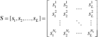
We assume the MIMO channel is memoryless and the MIMO system operates over a slowly-varying flat-fading MIMO channel. The transmit vector has L frame length at each antenna. The N_t × L space time codeword matrix is defined as follows:

(8.14)

and the MIMO channel matrix is given as (8.2). The maximum likelihood decoding scheme and perfect CSI are assumed at the receiver. Thus, the receiver has the following decision metric:

(8.15)

The ML decoder finds the codewords to minimize (8.15). We can calculate the Pairwise Error Probability (PEP) that the receiver decides erroneously as follows:

(8.16)

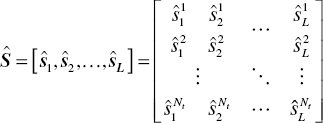
where Ŝ is the estimated erroneous sequence as follows:

(8.17)

and d²(S, Ŝ) is the modified Euclidean distance as follows:

(8.18)

where H is channel response sequences at each time as follows:

(8.19)

In (8.16), Q( ) is the complementary error function and σ is standard deviation of Gaussian noise. We define the codeword difference matrix B(S, Ŝ) and codeword distance matrix A(S, Ŝ) as follows:

(8.20)

and

(8.21)

(8.22)

where is complex conjugate. After simple manipulations [7], the modified Euclidean distance (8.18) is rewritten as follows:

(8.23)

where because a slow fading channel is assumed and channel gains at each frame are constant as follows:

(8.24)

The matrix A(S, Ŝ) is written as follows:

(8.25)

where Λ is a diagonal matrix as follows:

(8.26)

and V is an orthonormal matrix . The row vectors of V are the eigenvectors of A(S, Ŝ). Let , we express the term as follows:

(8.27)

Thus, (8.23) is rewritten as follows:

(8.28)

and (8.16) is rewritten using (8.28) as follows:

(8.29)

For Rayleigh fading [7], the upper bound of PEP is written as follows:

(8.30)

At a high SNR, we express the term as follows:

(8.31)

and (8.30) is simplified as follows:

(8.32)

where r is the rank of A(S, Ŝ). From (8.32), we can achieve diversity gain of rN_r and coding gain of . In other words, diversity gain is the exponent of PEP upper bound and coding gain is independent of SNR in PEP upper bound. Thus, we design to maximize diversity gain through maximizing the rank of a codeword difference matrix and then maximize coding gain through maximizing the minimum product of the Euclidean distance (or ). Both diversity gain and coding gain affect BER versus SNR performance curve differently. The diversity gain changes the slope of BER curve and the coding gain shifts it horizontally. A larger diversity gain and a greater coding gain make it more a negative slope and a larger left shift, respectively. Now, we define three design criteria for the space time coding in slow Rayleigh fading. The first design criterion is the rank criterion. The maximum diversity N_tN_r can be achieved if a codeword difference matrix B(S, Ŝ) has full rank for any two codeword vector sequences S and Ŝ. If it has the minimum rank r over two tuples of distinct codeword vector sequences, the diversity is rN_r. The second design criterion is about coding gain. Since the determinant of A(S, Ŝ) is the product of the eigenvalues, we calculate the determinant and call it the determinant criterion. Assume rN_r is the target diversity gain. We should maximize the minimum determinant of A(S, Ŝ) along the pairs of distinct codewords with the minimum rank. Therefore, we can minimize the PEP. This determinant criterion is related to coding gain but does not calculate an accurate coding gain. Thus, this criterion should be considered as one design rule of the space time coding. In Ref. [8], one more design criterion was discussed. The third design criterion is the trace criterion. In order to maximize the minimum Euclidean distance among all possible codewords, the minimum trace of A(S, Ŝ) should be maximized.

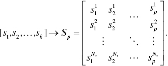
In Chapter 5, a 2 × 1 simple transmit diversity scheme by Alamouti was discussed. He extended his scheme to 2 × N_r codes and achieved a diversity order of 2N_r where a diversity order simply means the number of independent signal paths between a transmitter and a receiver. After that, V. Tarokh et al. [9, 10] generalized the simple transmit diversity scheme using orthogonal designs. Thus, STBCs with any number of antennas can be constructed and they achieve a full diversity. A generalized STBC is defined by a p × N_t transmission matrix S_p which generates N_t parallel signal sequences with the length p and whose elements are linear combinations of the k modulated signals (s₁, s₂, …, s_k) and their conjugates . The data rate of the STBC is defined as k/p. In a STBC encoder, the k modulated signal is encoded by a p × N_t transmission matrix S_p as follows:

(8.33)

In (8.33), S_p is constructed to satisfy

(8.34)

where c and I_p are constant and an identity matrix, respectively. The STBC can achieve a full diversity order of pN_r if S_p satisfies (8.34). When s_i is real and p is equal to N_t, then S₂, S₄, and S₈ are defined as follows [9]:

(8.35)

(8.36)

and

(8.37)

When s_i is complex, S_p construction is similar to the construction when it is real. The elements of S_p contain their conjugates and and are defined as follows [9]:

(8.38)

and

(8.39)

In the p × N_t transmission matrix S_p, each row represents a time slot and each column represents a transmit antenna. Thus, the code rate of is 1 and the code rate of is 1/2.

The STTCs are able to mitigate the effects of fading and provide us with a significant performance improvement. Now, we discuss the STTC design. The STTC encoder is similar to the TCM encoder. Figure 8.4 illustrates an STTC encoder.

As shown in Figure 8.4, the input sequence c_t is a block of information (or coded bits) at time t and is denoted by . The kth input sequence goes through the kth shift register and is multiplied by the STTC encoder coefficient set g^k. It is defined as follows:

(8.40)

Each represents an element of M-ary signal constellation set and v_m represents the memory order of the kth shift register. If QPSK modulation is considered, it has one of signal constellation set {0, 1, 2, 3}. The STTC encoder maps them into an M-ary modulated symbol and is denoted by . The output of the STTC encoder is calculated as follows:

(8.41)

where i = 1, 2, …, N_t. The outputs of the multipliers are summed modulo 2^m. The modulated symbols are transmitted in parallel through N_t transmit antennas. The total memory order of the STTC encoder is

(8.42)

and v_k is defined as follows:

(8.43)

The trellis state of the STTC encoder is 2^v. We assume that is the received signal at the received antenna j at time t, the receiver obtains perfect CSI, and the branch metric is calculated as the squared Euclidean distance between the actual received signal and the hypothesized received signals as follows:

(8.44)

The STTC decoder uses the Viterbi algorithm to select the path with the lowest path metric. In order to achieve full diversity, the STTC encoder requires a long memory and a large number of antennas. Thus, many states and branches of the Trellis diagram are needed. The complexity of the STTC decoder increases in proportion to them. This is one disadvantage of the STTC.

8.3 Example of STTC Encoding and Decoding

We consider a 2 × 2 space time trellis code with Gray coding QPSK and same coefficient set of the generator matrix as the Example 8.2. The input sequence [10, 01, 11, 01, 00] is encoded by the space time trellis encoder with the coefficient set of the generator matrix in Example 8.2. The output sequence is [02, 21, 13, 31, 10]. Figure 8.9 illustrates input/output sequences in the trellis diagram. We can observe a unique path.

In the trellis diagram, a branch label represents the input and output of the STTC encoder. means QPSK symbols transmitting via the transmit antenna 1 and 2. Figure 8.10 illustrates the STTC encoder and decoder.

As the decoder of the STTC, the Viterbi algorithm is used to perform maximum likelihood decoding. The branch metric of the trellis diagram is calculated using (8.44). For the 2 × 2 MIMO system with Gray coding QPSK, (8.44) is represented as follows:

(8.45)

where and represent in-phase components of the received QPSK signal and and represent quadrature-phase components of the received QPSK signal. Figure 8.11 illustrates Gray coding QPSK signal constellation.

In the receiver, we assume the received symbols and the estimated 2 × 2 MIMO channel gains as shown in Table 8.1. Unlike the Viterbi algorithm, the STTC decoder needs to estimate MIMO channel gains.

Time slot	Transmitted symbols	MIMO channel gain	Received symbols
1	02 ↔ (+0.7 +0.7j, −0.7 −0.7j)		(+0.98 +1.21j, −0.87 −0.95j)
2	21 ↔ (−0.7 −0.7j, −0.7 +0.7j)		(+0.75 +1.2j, −1.59 −1.22j)
3	13 ↔ (−0.7 +0.7j, +0.7 −0.7j)		(+0.93 +0.82j, −0.75 +0.12j)
4	31 ↔ (+0.7 −0.7j, −0.7 +0.7j)		(+1.25 +0.77j, −0.86 −0.97j)
5	10 ↔ (−0.7 +0.7j, +0.7 +0.7j)		(+0.81 +0.71j, −0.68 −0.79j)

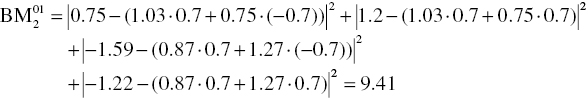
As the first step of STTC decoding, the branch metrics are calculated as follows:

At time 1,

At time 2,

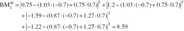
At time 3,

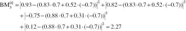
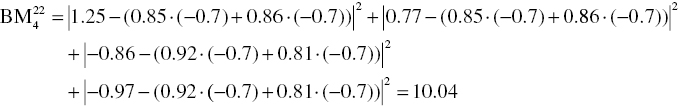
At time 4,

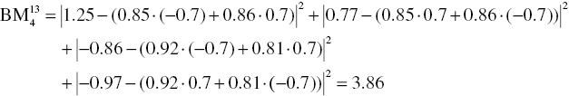
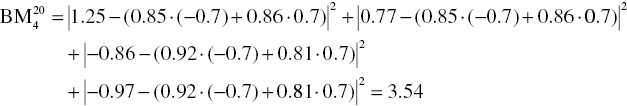
At time 5,

Figure 8.12 summarizes the branch metric calculations on the trellis diagram.

As the next step, the path metrics are calculated as follows:

At time 1,

At time 2,

At time 3,

At time 4,

At time 5,

Figure 8.13 summarizes the path metric calculations on the Trellis.

Based on path metric calculations, the traceback is carried out and the most likely path is found. As we can observe one unique path in Figure 8.14, the decoded sequence of STTC decoding is [10 01 11 01 00]. This is same as the input sequence of STTC encoder. We can check whether the STTC is able to correct a symbol error. If there is no the smallest path metric at each time, namely we have more than two minimum path metrics at each time, one path are selected arbitrarily. Similar to the Viterbi algorithm, a normalization process is needed to avoid overflow if the packet length is long.

A hardware implementation of the STTC encoder and decoder is similar to the convolutional encoder and Viterbi decoder. The encoder of the STTC can be implemented by a shift register, modulo adder/multiplier, and memory. The decoder of the STTC is composed of branch metric calculation, path metric calculation, normalization, traceback, and channel estimation. Among the components of the STTC decoder, channel estimation is a different part from the Viterbi decoder and it is a critical part to decide STTC performance.

8.4 Spatial Multiplexing and MIMO Detection Algorithms

Space time coding we discussed in the previous section provides us with a better link reliability due to a better diversity and coding gain. It transmits same symbols multiple times via different antennas and time slots. Thus, it cannot achieve multiplexing gain. Multiplexing gain means the maximum number of symbols which can be transmitted simultaneously at the same radio resource without additional power or bandwidth. A spatial multiplexing technique transmits multiple data streams via different transmit antennas in the same time and frequency. The received signal includes the multiple data streams and each transmitted data stream is extracted from the received signal. Thus, the spatial multiplexing technique can achieve a high multiplexing gain and increase a high channel capacity. However, the receiver complexity becomes very high. In this section, we review several MIMO detection algorithms and focus on one practical solution. Maximum likelihood (ML) detection is an optimal solution but the complexity exponentially grows according to the number of antennas. Thus, the application is limited at less than 4 antennas. For other applications, sub-optimal algorithms such as Matched filter (MF), Zero-forcing (ZF), Minimum Mean Square Error (MMSE), and Successive Interference Cancellation (SIC) (or BLAST) are practically considered. Sphere Decoding (SD) [11] and Fixed Sphere Decoding (FSD) [12] can provide near ML detection performance. Thus, it attracts many MIMO system designers’ attention. Figure 8.15 illustrates classification of MIMO detection algorithms.

Consider a spatial multiplexing system with N_t transmit antennas and N_r receive antennas and assume N_r ≥ N_t. The received signal r (N_r × 1 column vector) can be expressed as follows:

(8.46)

where H, s, and n represent N_r × N_t MIMO channel matrix, N_t × 1 transmit signal, and N_r × 1 white Gaussian noise vector, respectively. The element of r, r_j, is expressed as a superposition of all elements of s. Figure 8.16 illustrates the MIMO system for spatial multiplexing.

The maximum likelihood detection is to find the most likely ŝ as follows:

(8.47)

where denotes the norm of the matrix. The most likely ŝ is an element of set S. Thus, it is simple solution to search all possible elements of set S and select one to satisfy (8.47). This is known as nondeterministic polynomial (NP) hard problem. The complexity increases exponentially according to the number of transmit antennas and the modulation order. Linear detection techniques such as MF, ZF, and MMSE use a MIMO channel inversion. The transmitted symbol estimation is calculated by the MIMO channel version, multiplication, and quantization. The MF detection technique is one of the simplest detection techniques as follows:

(8.48)

where Qtz( ) represents quantization. The estimated symbols are obtained by multiplying the received symbols by Hermitian operation of the MIMO channel matrix. The ZF detection technique uses the pseudo-inverse of the MIMO channel matrix. When the MIMO channel matrix is square (N_t = N_r) and invertible, the estimated symbols by the ZF detection is expressed as follows:

(8.49)

When the MIMO channel matrix is not square (N_t ≠ N_r), it is expressed as follows:

(8.50)

As we can observe from (8.49) and (8.50), the ZF detection technique forces amplitude of interferers to be zero with ignoring a noise effect. Thus, the MMSE detection technique considering a noise effect provides a better performance than the ZF detection technique. The MMSE detection technique minimizes the mean-squared error. It is expressed as follows:

(8.51)

where I and N₀ represent an identity matrix and a noise. As we can observe from (8.51), an accurate estimation of the noise is required. If the noise term N₀ is equal to zero, the MMSE detection technique is same as the ZF detection technique. In linear detections, an accurate estimation of the MIMO channel matrix is an essential part and these detections are useful at a high SNR. The SIC detection technique is located between ML detection and linear detection. It provides a better performance than linear detections. The SIC detection uses nulling and cancellation to extract the transmitted symbols from the received symbols. When one layer (a partial symbol sequence from one transmit antenna) is detected, an estimation of the transmitted layer is performed by subtracting from the detected layers in the previous time. The nulling and cancellation are carried out until all layers are detected. The SIC detection shows us good performance at a low SNR. One disadvantage is that the SIC suffers from error propagation. When a wrong decision is made in any layer, the wrong decision affects the other layers. Thus, the ordering technique is used to minimize the effect of error propagation. In the nulling and cancellation with the ordering technique, the first symbol with a high SNR is transmitted as the most reliable symbol. Then, the symbols with a lower SNR are transmitted. Both the linear detection and the SIC detection cannot achieve the ML detection performance even if they have a lower complexity than the ML detection. Thus, many MIMO system designers pay attention to the SD algorithm which can achieve near ML detection performance with a lower complexity than the exhaustive search. The basic idea of the SD algorithm is very simple. The ML detection searches all possible elements of the transmitted symbols but the SD algorithm searches a finite number of symbols within sphere radius centered at the received symbol vector. The SD algorithm is expressed as follows:

(8.52)

Consider a simple example about a two transmit antennas system with BPSK. The lattice points are shown in Figure 8.17.

In this figure, the candidate symbol represents (BPSK symbol from antenna 1, BSPK symbol from antenna 2) [+1, +1], [−1, +1], [−1, −1], and [+1, −1], respectively. The ML detection searches all possible lattice points (ŝ₁, ŝ₂, ŝ₃, and ŝ₄) but the SD algorithm searches only some lattice points (ŝ₂, ŝ₃) in a sphere radius centered at the received symbol vector r. Thus, the computational complexity can be significantly reduced and the performance of the SD algorithm is almost same as the ML detection. The SD detection selects the lattice point ŝ₂ due to the closest one from the received symbol. This is same selection of the ML detection. As we can observe from (8.52), the sphere radius is very important to performance and complexity. If the radius is too small, we may not have any candidate lattice points in the circle so that the performance may be worse. If the radius is too large, we may search too many candidate lattice points so that the complexity may increase very much. We reformulate (8.52) using QR decomposition and build a decision tree [13]. As we discussed in Chapter 5, the channel matrix H is expressed as follows:

(8.53)

where Q and R denote an orthogonal matrix and an upper triangular matrix, respectively. Thus, (8.52) is rewritten as follows:

(8.54)

(8.55)

where . An iterative solution is used in order to solve (8.55). When considering , (8.55) is expressed as a Partial Euclidean Distance (PED). Thus, we deal with the following equation:

(8.56)

(8.57)

where T_i(s⁽ⁱ⁾) represents the cumulative PED at level i from levels i + 1 and . e_i(s⁽ⁱ⁾) represents the distance from level i + 1 to level i. i represents each level of a tree and the total number of levels are same as the number of transmit antennas. Each node means signal constellation order. is a sequence of symbols until level i. s⁽¹⁾ at level 1 means the total sequence of the symbol. Figure 8.18 illustrates an SD search tree with N_t transmit antennas and M-ary modulation.

The complexity of the SD detection algorithm is not fixed because the node visiting depends on channel condition. In addition, the SD algorithm is based on sequential search so that it is difficult to use pipelining techniques and system throughput is low. On the other hand, the complexity of FSD detection algorithm is fixed because it searches only a fixed number of nodes. The architecture is suitable for pipelining techniques. In the hardware implementation point of view, this is an important advantage. For example, one symbol from an antenna with a better channel condition or a higher SNR will be correctly detected. Thus, we do not need to search the other possible symbols. The FSD algorithm calculates a fixed number of transmitted symbols which are subset of all possible transmitted symbols. If the number of branches we consider in the FSD algorithm is [s₁ s₂ s₃] = [1 2 1] (e.g., we decide s₁ = −1 and s₃ = −1 in advance.) in Example 8.3, the FSD search tree can be drawn as shown in Figure 8.21.

We calculate only two paths in the FSD search tree. The selection of the fixed number of the transmitted symbol affects complexity and performance. They are trade-off relationship. Figure 8.22 illustrates the FSD hardware architecture.

The FSD hardware architecture needs the received symbol r and the channel matrix H as the inputs where we assume H is perfectly known in the receiver. In the channel ordering block, the detection ordering is decided with satisfying the following relationship:

(8.58)

where E(n_i) is the distribution of candidates (or the visited nodes at level i). The columns of the channel matrix H are ordered iteratively. For the received symbol with the lowest SNR, we select the maximum number of branches (same as modulation order) at the level. For the received symbol with a high SNR, we select smaller number of branches at the level. The QR decomposition block can be implemented by COordinate Rotation DIgital Computer (CORDIC) [14]. We obtain an upper triangular matrix R and from QR decomposition. PEDs are calculated at each level block. In decision block, one node with the minimum PED is selected and the transmitted symbols ŝ are estimated as the output of the FSD.

In this chapter, we mainly investigated two MIMO techniques: space time coding and spatial multiplexing. Space time coding shows us good performance at a low SNR and spatial multiplexing shows us good performance at a high SNR. Thus, adaptive MIMO technique combining both techniques would be a good solution. Figures 8.23 and 8.24 illustrate adaptive MIMO architecture and its performance, respectively.

8.5 Problems

1. 8.1. Describe the MIMO antenna design considerations for indoor and outdoor applications.
2. 8.2. SVD is fully parallelizing MIMO channel but each subchannel has different gain. On the other hands, QR decomposition has equal diagonal value but each subchannel is not fully parallelizing. Compare the BER performance of both SVD beamforming and QR decomposition beamforming.
3. 8.3. Compare the diversity gain of both Alamouti scheme and V-BLAST for 2 × 2 and 4 × 4 MIMO channels.
4. 8.4. Consider the space time code and any two distinct codeword by (8.39). Find the diversity gain.
5. 8.5. Describe the encoding and decoding process of 2 × 2 Alamouti scheme.
6. 8.6. Consider the 4 × 4 MIMO system in Rayleigh fading channel. Compare the BER performance of ZF, MMSE, and SIC detection algorithm.
7. 8.7. Adaptive MIMO performance is shown in Figure 8.24. Find the switching point from STC to SM.
8. 8.8. Compare the MIMO schemes in LTE and WiMAX.

References

1. [1] R. Janaswamy “Effect of Element Mutual Coupling on the Capacity of Fixed Length Linear arrays,” IEEE Antennas and Wireless Propagation Letters, vol. 1, no. 1, pp. 157–160, 2002.
2. [2] M. A. Jensen and R. W. Wallace, “A Review of Antennas and Propagation for MIMO Wireless Communications,” IEEE Transactions on Antennas and Propagation, vol. 52, no. 11, 2004.
3. [3] S. W. Ellingson, “Antenna Design and Site Planning Considerations for MIMO,” Proceedings of IEEE the 62nd Vehicular Technology Conference (VTC Fall 2005), pp. 1718–1722, September 2005.
4. [4] V. Tarokh and H. Jafarkhani, “A Differential Detection Scheme for Transmit Diversity,” IEEE Journal on Selected Areas in Communications, vol. 18, no. 7, 2000.
5. [5] I. E. Telatar, “Capacity of Multi-Antenna Gaussian Channels,” European Transactions on Telecommunications and Related Technologies, vol. 10, no.6, pp.586–596, 1999.
6. [6] D. Tse and P. Viswanath, Fundamentals of Wireless Communication, Cambridge University Press, Cambridge, 2005.
7. [7] V. Tarokh, N. Seshadri, and A. R. Calderbank, “Space-Time Codes for High Data Rate Wireless Communication: Performance Criterion and Code Construction,” IEEE Transactions on Information Theory, vol. 44, no. 2, 1998.
8. [8] D. M. Ionescu, “New Results on Space-Time Code Design Criteria,” Proceedings of IEEE Wireless Communications and Networking Conference (WCNC’99), vol. 2, pp. 684–687, 1999.
9. [9] V. Tarokh, H. Jafarkhani, and A. R. Calderbank, “Space-time Block Coding from Orthogonal Designs,” IEEE Transactions on Information Theory, vol. 45, pp. 1456–1467, 1999.
10. [10] V. Tarokh, H. Jafarkhani, and A. R. Calderbank, “Space-time Block Doing for Wireless Communications: Performance Results,” IEEE Journal on Selected Areas in Communications, vol. 17, no. 3, pp. 451–460, 1999.
11. [11] E. Viterbo and J. Boutros, “A Universal Lattice Code Decoder for Fading Channels,” IEEE Transactions on Information Theory, vol. 45, no. 5, pp. 1639–1642, 1999.
12. [12] L. G. Barbero and J. S. Thompson, “Fixing the Complexity of the Sphere Decoder for MIMO Detection,” IEEE Transactions on Wireless Communications, vol. 7, no. 6, pp. 2131–2142, 2008.
13. [13] B. Hassibi and H. Vikalo, “On the Sphere-Decoding Algorithm. Part I, Expected Complexity,” IEEE Transactions on Signal Processing, vol. 53, no. 8, pp. 2806–2818, 2005.
14. [14] J. E. Volder, “The CORDIC Trigonometric Computing Techniques,” IRE Transactions on Electronic Computers, vol. EC-8, no. 3, pp. 330–334, 1959.