
Chapter 5
Stochastic Enumeration Method
5.1 Introduction
In this chapter, we introduce a new generic sequential importance sampling (SIS) algorithm, called stochastic enumeration (SE) for counting #P problems. SE represents a natural generalization of one-step-look-ahead (OSLA) algorithms. We briefly introduce these concepts here and defer explanation of the algorithms in detail to the subsequent sections.
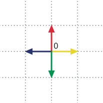
Consider a simple walk in the integer lattice ![]() . It starts at the origin (0,0) and it repeatedly takes unit steps in any of the four directions, North (N), South (S), East (E), or West (W). For instance, an 8-step walk could be
. It starts at the origin (0,0) and it repeatedly takes unit steps in any of the four directions, North (N), South (S), East (E), or West (W). For instance, an 8-step walk could be
We impose the condition that the walk may not revisit a point that it has previously visited. These walks are called self-avoiding walks (SAW). SAWs are often used to model the real-life behavior of chain-like entities such as polymers, whose physical volume prohibits multiple occupation of the same spatial point. They also play a central role in modeling of the topological and knot-theoretic behavior of molecules such as proteins.
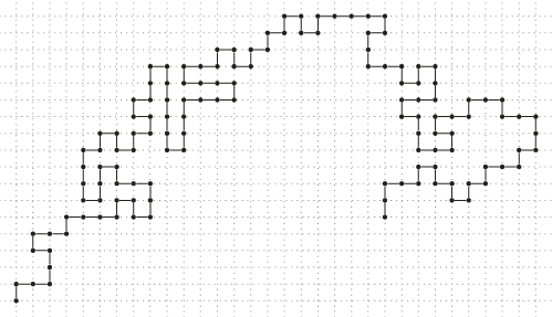
Clearly, the 8-step walk above is not a SAW inasmuch as it revisits point ![]() . Figure 5.1 presents an example of a 130-step SAW. Counting the number of SAWs of length
. Figure 5.1 presents an example of a 130-step SAW. Counting the number of SAWs of length ![]() is a basic problem in computational science for which no exact formula is currently known. The problem is conjectured to be complete in #P
is a basic problem in computational science for which no exact formula is currently known. The problem is conjectured to be complete in #P![]() , that is, the version of #P in which the input consists of binary symbols, see [78] [120]. Though many approximating methods exist, the most advanced algorithms are the pivot ones. They can handle SAWs of size
, that is, the version of #P in which the input consists of binary symbols, see [78] [120]. Though many approximating methods exist, the most advanced algorithms are the pivot ones. They can handle SAWs of size ![]() , see [30] [82]. For a good recent survey, see [121].
, see [30] [82]. For a good recent survey, see [121].
Figure 5.1 SAW of length 130.
We consider randomized algorithms for counting SAWs of length at least some given ![]() , say
, say ![]() . A natural, simple algorithm goes as follows: it chooses at the current end point of the walk randomly one of the feasible neighbors and moves to it. This is done until either a path of length of
. A natural, simple algorithm goes as follows: it chooses at the current end point of the walk randomly one of the feasible neighbors and moves to it. This is done until either a path of length of ![]() is obtained or there is no available neighbor. In the latter case, we say that the walk is trapped, or that the algorithm gets stuck. Then, the algorithm returns a zero counting value. Otherwise it returns the product of the consecutive numbers of available neighbors at each step. This is repeated
is obtained or there is no available neighbor. In the latter case, we say that the walk is trapped, or that the algorithm gets stuck. Then, the algorithm returns a zero counting value. Otherwise it returns the product of the consecutive numbers of available neighbors at each step. This is repeated ![]() times independently; the average is taken as an estimator of the counting problem. Typical features of this algorithm are that
times independently; the average is taken as an estimator of the counting problem. Typical features of this algorithm are that
- it runs a single path, or trajectory;
- it is sequential, because it moves iteratively from point to point;
- it is randomized, because the next point is chosen at random (if possible);
- it is OSLA, because in each iteration it decides how to continue by considering only its nearest feasible points.
Note that any feasible SAW ![]() of length
of length ![]() has a positive probability
has a positive probability ![]() of being constructed by this simple algorithm. The main two drawbacks of the algorithm are that
of being constructed by this simple algorithm. The main two drawbacks of the algorithm are that
- the pdf
 is nonuniform on the space of all feasible SAWs of length
  , which causes high variance of the associated estimator;
 - it gets stuck easily for large
 , cf. [79].
To overcome the first drawback, we suggest in Section 5.2.2 to run multiple trajectories in parallel. This will typically reduce the variance substantially. To eliminate the second drawback, we ask an oracle at each iteration how to continue in order that the walk not be trapped too early. That is, the oracle can foresee which feasible nearest neighbors lead to a trap and which do not. As an example, consider constructing a SAW of length ![]() , then Figure 5.2 shows how the OSLA algorithm can lead to a trap after 15 iterations.
, then Figure 5.2 shows how the OSLA algorithm can lead to a trap after 15 iterations.
Figure 5.2 SAW trapped after 15 iterations.
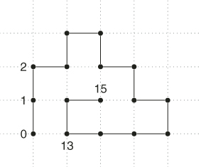
However, an oracle would, say, after 13 iterations continue to the South rather than to the North. We call such oracle-based algorithms ![]() -step-look-ahead (
-step-look-ahead (![]() SLA), because instances are generated iteratively while having information how to continue without being trapped before the last iteration or step. Thus, it has the advantage of not losing trajectories. Notice that in our example this
SLA), because instances are generated iteratively while having information how to continue without being trapped before the last iteration or step. Thus, it has the advantage of not losing trajectories. Notice that in our example this ![]() SLA algorithm still runs single trajectories, resulting again in high variances of its associated estimator, see Section 5.2.1. Next, we propose to run multiple trajectories in combination with the
SLA algorithm still runs single trajectories, resulting again in high variances of its associated estimator, see Section 5.2.1. Next, we propose to run multiple trajectories in combination with the ![]() SLA oracle. We call this method stochastic enumeration (SE), and we will provide the details and analysis in Section 5.3.
SLA oracle. We call this method stochastic enumeration (SE), and we will provide the details and analysis in Section 5.3.
Summarizing, the features of SE are
- It runs multiple trajectories in parallel, instead of a single one; by doing so, the samples from
 become close to uniform.
 - It employs
 -step-look-ahead algorithms (oracles); this is done to overcome the generation of zero outcomes of the estimator.
As a side effect, SE reduces a difficult counting problem to a set of simple ones, applying at each step an oracle. Furthermore, we note that, in contrast to the conventional splitting algorithm of Chapter 4, there is less randomness involved in SE. As a result, it is typically faster than splitting.
A main concern of using oracles deals with its computational complexity. At each iteration, we apply a decision-making oracle because we are only interested in which direction we can continue generating the path without being trapped somewhere later. Thus, we propose directions and wait for yes-no decisions of the oracle. Hence, for problems for which polynomial time decision-making algorithms exist, SE will be applicable and runs fast.
It is interesting to note that there are many problems in computational combinatorics for which the decision-making is easy (polynomial) but the counting is hard (#P-complete). For instance,
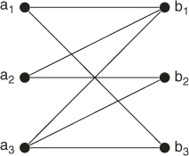
It was known quite a long time ago that finding a perfect matching for a given bipartite (undirected) graph ![]() can be solved in polynomial
can be solved in polynomial ![]() time, while the corresponding counting problem, “How many perfect matchings does the given bipartite graph have?” is already #P-complete. The problem of counting the number of perfect matchings is known to be equivalent to the computation of the permanent of a matrix [119].
time, while the corresponding counting problem, “How many perfect matchings does the given bipartite graph have?” is already #P-complete. The problem of counting the number of perfect matchings is known to be equivalent to the computation of the permanent of a matrix [119].
Similarly, there is a trivial algorithm for determining whether a given DNF form of the satisfiability problem is true. Indeed, in this case we have to examine each clause, and if a clause is found that does not contain both a variable and its negation, then it is true, otherwise it is not. However, the counting version of this problem is #P-complete.
Many #P-complete problems have a fully polynomial-time randomized approximation scheme (FPRAS), which, informally, will produce with high probability an approximation to an arbitrary degree of accuracy, in time that is polynomial with respect to both the size of the problem and the degree of accuracy required [88]. Jerrum, Valiant, and Vazirani [60] showed that every #P-complete problem either has an FPRAS or is essentially impossible to approximate; if there is any polynomial-time algorithm that consistently produces an approximation of a #P-complete problem that is within a polynomial ratio in the size of the input of the exact answer, then that algorithm can be used to construct an FPRAS.
The use of fast decision-making algorithms (oracles) for solving NP-hard problems is very common in Monte Carlo methods; see, for example,
- Karger's paper [64], which presents an FPRAS for network unreliability based on the well-known DNF polynomial counting algorithm of Karp and Luby [65].
- The insightful monograph of Gertsbakh and Shpungin [41] in which Kruskal's spanning trees algorithm is used for estimating network reliability.
Our main strategy is as in [41]: use fast polynomial decision-making oracles to solve #P-complete problems. In particular, one can easily incorporate into SE the following:
- The breadth-first-search procedure or Dijkstra's shortest path algorithm [32] for counting the number of paths in the networks.
- The Hungarian decision-making assignment problem method [74] for counting the number of perfect matchings.
- The decision-making algorithm for counting the number of valid assignments in 2-SAT, developed in Davis et al. [35] [36].
- The Chinese postman (or Eulerian cycle) decision-making algorithm for counting the total number of shortest tours in a graph. Recall that in a Eulerian cycle problem, one must visit each edge at least once.
The remainder of this chapter is organized as follows. Section 5.2 presents some background on the classical OSLA algorithm and its extensions: (i) using an oracle and (ii) using multiple trajectories. Section 5.3 is the main discussion; it deals with both OSLA extensions simultaneously, resulting in the SE method.
Section 5.4 deals with applications of SE to counting in #P-complete problems, such as counting the number of trajectories in a network, number of satisfiability assignments in a SAT problem, and calculating the permanent. Here we also discuss how to choose the number of parallel trajectories in the SE algorithm. Unfortunately, there is no ![]() SLA polynomial oracle for SAW. Consequently, SE is not directly applicable to SAW and we must resort to its simplified (time-consuming) version. This section describes the algorithms; some corresponding numerical results are given in Section 5.5. There we also show that SE outperforms the splitting method discussed in Chapter 4 and SampleSearch method of Gogate and Dechter [56] [57]. Our explanation for this is that SE is based on SIS (sequential importance sampling), whereas its two counterparts are based merely on the standard (nonsequential) importance sampling.
SLA polynomial oracle for SAW. Consequently, SE is not directly applicable to SAW and we must resort to its simplified (time-consuming) version. This section describes the algorithms; some corresponding numerical results are given in Section 5.5. There we also show that SE outperforms the splitting method discussed in Chapter 4 and SampleSearch method of Gogate and Dechter [56] [57]. Our explanation for this is that SE is based on SIS (sequential importance sampling), whereas its two counterparts are based merely on the standard (nonsequential) importance sampling.
5.2 OSLA Method and Its Extensions
Let ![]() be our counting quantity, such as,
be our counting quantity, such as,
- the number of satisfiability assignments in a SAT problem with
 literals;
 - the number of perfect matchings (permanent) in a bipartite graph with
 nodes;
 - the number of SAWs of length
 .
.
We assume, similarly to in Chapter 4, that ![]() is a subset of some larger but finite sample space
is a subset of some larger but finite sample space ![]() . Let
. Let ![]() be the uniform pdf and
be the uniform pdf and ![]() some arbitrary pdf on
some arbitrary pdf on ![]() that is positive for all
that is positive for all ![]() , and suppose that we generate a random element
, and suppose that we generate a random element ![]() using these pdfs; then we can write
using these pdfs; then we can write
This special case of importance sampling says that, when we generate a random element ![]() using pdf
using pdf ![]() , we define the (single-run) estimator
, we define the (single-run) estimator
As usual, we take the sample mean of ![]() independent retrials. Clearly, we obtain an unbiased estimator of the counting quantity,
independent retrials. Clearly, we obtain an unbiased estimator of the counting quantity, ![]() . Furthermore, it is easy to see that the estimator has zero variance if and only if
. Furthermore, it is easy to see that the estimator has zero variance if and only if ![]() , the uniform pdf on the target set.
, the uniform pdf on the target set.
Next, we assume additionally that the sample space ![]() is contained in some
is contained in some ![]() -dimensional vector space; that is, samples
-dimensional vector space; that is, samples ![]() can be represented by vectors of
can be represented by vectors of ![]() components. For instance, consider the problem of counting SAWs of length
components. For instance, consider the problem of counting SAWs of length ![]() . Each sample is a simple walk
. Each sample is a simple walk ![]() where the individual components
where the individual components ![]() are points in the integer two-dimensional lattice. Then we might consider to decompose the importance sampling pdf
are points in the integer two-dimensional lattice. Then we might consider to decompose the importance sampling pdf ![]() as a product of conditional pdfs:
as a product of conditional pdfs:
5.1 ![]()
The importance sampling simulation of generating a random sample ![]() is executed by generating sequentially the next component
is executed by generating sequentially the next component ![]() (
(![]() ) given the previouscomponents
) given the previouscomponents ![]() . This method is called sequential importance sampling (SIS); see Section 5.7 in [108] for details in a general setting.
. This method is called sequential importance sampling (SIS); see Section 5.7 in [108] for details in a general setting.
In particular, we apply a specific version of SIS, the OSLA procedure due to Rosenbluth and Rosenbluth [97], which was originally introduced for SAWs, as we described in the introductory section. Below, we give more details of the consecutive steps of the OSLA procedure, where we have in mind generating a sample ![]() for problems in which
for problems in which ![]() represents a path of consecutive points
represents a path of consecutive points ![]() . The first point
. The first point ![]() of the path is fixed and constant for all paths, called the origin. For example, in the SAW problem,
of the path is fixed and constant for all paths, called the origin. For example, in the SAW problem, ![]() , or in a network with source
, or in a network with source ![]() and sink
and sink ![]() ,
, ![]() .
.
Note that the OSLA procedure defines the SIS pdf:
5.3 
The OSLA counting algorithm now follows.
5.4 
The efficiency of the OSLA method deteriorates rapidly as ![]() becomes large. For example, it becomes impractical to simulate random SAWs of length more than 200. This is due to the fact that, if at any step
becomes large. For example, it becomes impractical to simulate random SAWs of length more than 200. This is due to the fact that, if at any step ![]() the point
the point ![]() does not have unoccupied neighbors (
does not have unoccupied neighbors (![]() ), then
), then ![]() is zero and it contributes nothing to the final estimate of
is zero and it contributes nothing to the final estimate of ![]() .
.
As an example, consider again Figure 5.2, depicting a SAW trapped after 15 iterations. One can easily see that the corresponding values ![]() of each of the 15 points are
of each of the 15 points are
![]()
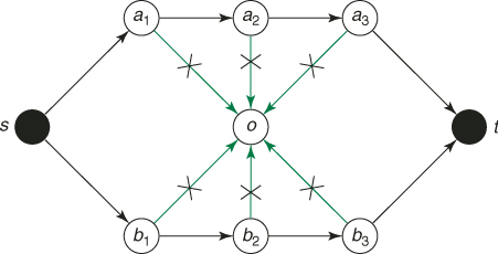
As for another situation where OSLA can be readily trapped, consider a directed graph in Figure 5.3 with source ![]() and sink
and sink ![]() . There are two ways from
. There are two ways from ![]() to
to ![]() , one via nodes
, one via nodes ![]() and another via nodes
and another via nodes ![]() . Figure 5.3 corresponds to
. Figure 5.3 corresponds to ![]() . Note that all nodes besides
. Note that all nodes besides ![]() and
and ![]() are directly connected to a central node
are directly connected to a central node ![]() , which has no connection with
, which has no connection with ![]() . Clearly, in this case, most of the random walks (with probability
. Clearly, in this case, most of the random walks (with probability ![]() ) will be trapped at node
) will be trapped at node ![]() .
.
Figure 5.3 Directed graph.
5.2.1 Extension of OSLA:  SLA Method
A natural extension of the OSLA procedure is to look ahead more than one step. We consider only the case of looking all the way to the end, which we call the ![]() SLA method. This means that no path will be ever lost, and it implies that
SLA method. This means that no path will be ever lost, and it implies that ![]() , for all
, for all ![]() .
.
Consider, for example, the SAW in Figure 5.2. If we could use the ![]() SLA method instead of OSLA, we would rather move after step 13 (corresponding to point
SLA method instead of OSLA, we would rather move after step 13 (corresponding to point ![]() ) South instead of North. By doing so we would prevent the SAW being trapped after 15 iterations.
) South instead of North. By doing so we would prevent the SAW being trapped after 15 iterations.
For many problems, including SAWs, the ![]() SLA algorithm requires additional memory and computing power; for that reason, it has limited applications. There exists, however, a set of problems where
SLA algorithm requires additional memory and computing power; for that reason, it has limited applications. There exists, however, a set of problems where ![]() SLA can be implemented easily by using polynomial-time oracles. As mentioned, relevant examples are counting perfect matchings in a graph and counting the number of paths in a network.
SLA can be implemented easily by using polynomial-time oracles. As mentioned, relevant examples are counting perfect matchings in a graph and counting the number of paths in a network.
The ![]() SLA procedure does not differ much from the OSLA procedure. For completeness, we present it below.
SLA procedure does not differ much from the OSLA procedure. For completeness, we present it below.
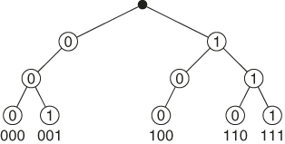
To see how ![]() SLA works in practice, consider a simple example following the main steps of the OSLA Algorithm 5.1.
SLA works in practice, consider a simple example following the main steps of the OSLA Algorithm 5.1.
![]()
Figure 5.5 presents the subtrees ![]() (in bold) generated by
(in bold) generated by ![]() SLA using the oracle.
SLA using the oracle.
![]()
As a comparison, the OSLA algorithm generates the valid combinations each with probability ![]() (with probability
(with probability ![]() OSLA is trapped). Hence the associated OSLA estimator has variance 15.
OSLA is trapped). Hence the associated OSLA estimator has variance 15.![]()
The main drawback of ![]() SLA Procedure 2 is that its SIS pdf
SLA Procedure 2 is that its SIS pdf ![]() is model dependent. Typically, it is far from the ideal uniform SIS pdf
is model dependent. Typically, it is far from the ideal uniform SIS pdf ![]() , that is,
, that is,
![]()
As a result, the estimator of ![]() has a large variance.
has a large variance.
To see the nonuniformity of ![]() , consider a 2-SAT model with clauses
, consider a 2-SAT model with clauses ![]() , where
, where ![]() Figure 5.6 presents the corresponding graph with four literals and
Figure 5.6 presents the corresponding graph with four literals and ![]() . In this case,
. In this case, ![]() , the zero variance pdf
, the zero variance pdf ![]() , whereas the SIS pdf is
, whereas the SIS pdf is

which is highly nonuniform.
Figure 5.6 A graph with four literals and ![]() .
.
To improve the nonuniformity of ![]() , we will run the
, we will run the ![]() SLA procedure in parallel by multiple trajectories. Before doing so, we present below for convenience a multiple trajectory version of the OSLA Algorithm 5.1 for SAWs.
SLA procedure in parallel by multiple trajectories. Before doing so, we present below for convenience a multiple trajectory version of the OSLA Algorithm 5.1 for SAWs.
5.2.2 Extension of OSLA for SAW: Multiple Trajectories
In this section, we extend the OSLA method to multiple trajectories and present the corresponding algorithm. For ease of referencing, we call it multiple OSLA. We provide it here for counting SAWs.
5.2.2.1 Multiple-OSLA Algorithm for SAW
Recall that a SAW is a sequence of moves in a lattice such that it does not visit the same point more than once. There are specially designed counting algorithms, for instance, the pivot algorithm [30]. Empirically we found that these outperform our multiple-OSLA algorithm; nevertheless, we present it below in the interest of clarity of representation and for motivational purposes.
For simplicity, we assume that the walk starts at the origin, and we confine ourselves to the two-dimensional integer lattice case. Each SAW is represented by a path ![]() , where
, where ![]() . A SAW of length
. A SAW of length ![]() has been given in Figure 5.1.
has been given in Figure 5.1.
- Full Enumeration. Select a small number
 , say
, say  and count via full enumeration all different SAWs of size
  starting from the origin
  . Denote the total number of these SAWs by
  and call them the elite sample. For example, for
  , the number of elites
  . Set the first level to
  . Proceed with the
  elites from level
  to the next one,
  , where
  is a small integer (typically
  or
or  ) and count via full enumeration all different SAWs at level
  . Denote the total number of such SAWs by
  . For example, for
  there are
  different SAWs.
 - Calculation of the First Weight Factor. Compute
5.5
and call it the first weight factor.
- Full Enumeration. Proceed with
 elites from iteration
  to the next level
  and derive via full enumeration all SAWs at level
  , that is, of all those SAWs that continue the
  paths resulting from the previous iteration. Denote by
  the resulting number of such SAWs.
 - Stochastic Enumeration. Select randomly without replacement
 SAWs from the set of
  ones and call this step stochastic enumeration.
 - Calculation of the
 -th Weight Factor. Compute
5.6
and call it the
 -th weight factor. Similar to OSLA, the weight factor
  can be both
  and
and  ; in case
 , we stop and deliver
  .
.
- Proceed with iteration
 and compute
- Call
 the point estimator of
  .
. - Since the number of levels is fixed,
 presents an unbiased estimator of
  (see [73]).
- Run Steps 1–3 for
 independent replications and deliver
as an unbiased estimator of
independent replications and deliver
as an unbiased estimator of  .
. - Call
 the multiple-OSLA estimator of
  .
.
A few remarks can be made:
- Typically, one keeps the number of elites
 in multiple OSLA fixed, say
  , while
  varies from iteration to iteration.
 - OSLA represents a particular case of multiple OSLA, when the number of elites is
 in all iterations.
 - In contrast to OSLA, which loses most of its trajectories (even for modest
 ), with multiple OSLA we can reach quite large levels, say
  , provided the number
  of elite samples is not too small, say
  in all iterations. Hence, one can generate very long random SAWs with multiple OSLA.
 - The sample variance of
 is
is
5.9
and the relative error is
5.10
- There is similarity with the splitting method of Chapter 4 in the sense that the whole state space is broken in smaller search spaces, in which the promising samples (elites) are chosen for prolongation.
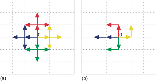
- Full Enumeration. We set
 and count (via full enumeration) all different SAWs of length
  starting from the origin
  . We have
  (see Figure 5.7). We proceed (again via full enumeration) to derive from the
  elites all SAWs of length
  (there are
  of them, see part (a) of Figure 5.8).
 - Calculation of the first weight factor. We have
 .
.
- Stochastic Enumeration. Select randomly without replacement
 elites from the set of
  ones (see part (b) of Figure 5.8).
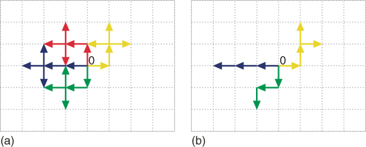
 - Full Enumeration. Proceed via full enumeration to determine all SAWs of length
 that extend the
  elites. There are
  of them, see part (a) of Figure 5.9.
 - Calculation of the second weight factor. We have
 .
.
Experiments with the multiple-OSLA algorithm for general counting problems, like SAT, indicated that this method is also susceptible to generating many zeros (trajectories of zero length); even for a relatively small model sizes. For this reason it has limited applications.
For example, consider a 3-SAT model with an adjacency matrix ![]() and
and ![]() . Running the multiple-OSLA Algorithm 5.2 with
. Running the multiple-OSLA Algorithm 5.2 with ![]() , we observed that it discovered all 15 valid assignments (satisfying all 80 clauses) only with probability
, we observed that it discovered all 15 valid assignments (satisfying all 80 clauses) only with probability ![]() . We found that, as the size of the models increases, the percentage of valid assignments goes rapidly to zero.
. We found that, as the size of the models increases, the percentage of valid assignments goes rapidly to zero.
5.3 SE Method
Here we present our main algorithm, called stochastic enumeration (SE), which extends both the ![]() SLA and the multiple-OSLA algorithms as follows:
SLA and the multiple-OSLA algorithms as follows:
- SE extends
 SLA in the sense that it uses multiple trajectories instead of a single one.
 - SE extends the multiple-OSLA Algorithm 5.2 in the sense that it uses an oracle at the Full Enumeration step.
We present SE for the models where the components of the vector ![]() are assumed to be binary variables, such as SAT, and where fast decision-making
are assumed to be binary variables, such as SAT, and where fast decision-making ![]() SLA oracles are available (see [35] [36] for SAT). Its modification to arbitrary discrete variables is straightforward.
SLA oracles are available (see [35] [36] for SAT). Its modification to arbitrary discrete variables is straightforward.
5.3.1 SE Algorithm
Consider the multiple-OSLA Algorithm 5.2 and assume for simplicity that ![]() and that at iteration
and that at iteration ![]() the number of elites is, say,
the number of elites is, say, ![]() . In this case, it can be seen that, in order to implement an oracle in the Full Enumeration step at iteration
. In this case, it can be seen that, in order to implement an oracle in the Full Enumeration step at iteration ![]() , we have to run it
, we have to run it ![]() times: 100 times for
times: 100 times for ![]() and 100 more times for
and 100 more times for ![]() . For each fixed combination of
. For each fixed combination of ![]() , the oracle can be viewed as an
, the oracle can be viewed as an ![]() SLA algorithm in the following sense:
SLA algorithm in the following sense:
- It sets first
 and then makes a decision (YES-NO path) for the remaining
  variables
  .
. - It sets next
 and then again makes a similar (YES-NO) decision for the same set
  .
.
- Full Enumeration. (Similar to Algorithm 5.2.) Let
 be the number corresponding to the first
  variables
  . Count via full enumeration all different paths (valid assignments in SAT) of size
  . Denote the total number of these paths (assignments) by
  and call them the elite sample. Proceed with the
  elites from level
  to the next one
  , where
  is a small integer (typically
  or
or  ) and count via full enumeration all different paths (assignments) of size
  . Denote the total number of such paths (assignments) by
  .
. - Calculation of the First Weight Factor. Same as in Algorithm 5.2.
- Full Enumeration. (Same as in Algorithm 5.2, except that it is performed via the corresponding polynomial time oracle rather than OSLA.) Recall that for each fixed combination of
 , the oracle can be viewed as an
  -step look-ahead algorithm in the sense that it
- Sets first
 and then makes a YES-NO decision for the path associated with the remaining
  variables
  .
. - Sets next
 and then again makes a similar (YES-NO) decision.
- Sets first
- Stochastic Enumeration. Same as in Algorithm 5.2.
- Calculation of the
 -th Weight Factor. (Same as in Algorithm 5.2.) Recall that, in contrast to multiple OSLA, where
  , here
  .
.
It follows that, if ![]() in all iterations, the SE Algorithm 5.3 will be exact.
in all iterations, the SE Algorithm 5.3 will be exact.
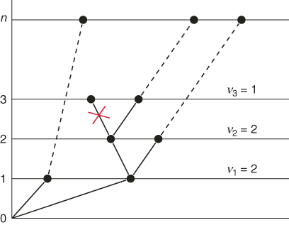
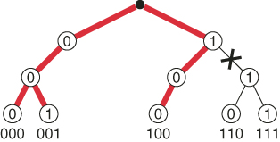
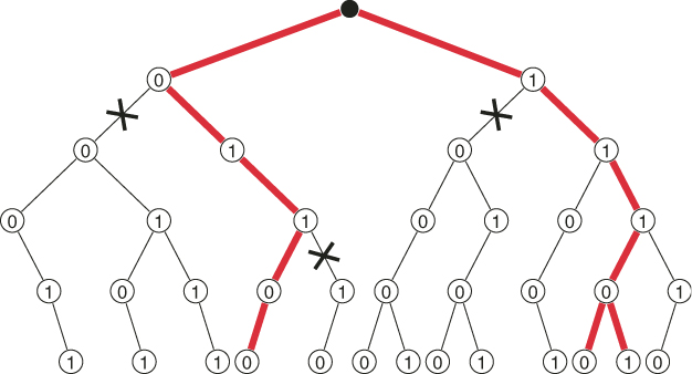
Figure 5.11 presents the dynamics of the SE Algorithm 5.3 for the first three iterations in a model with ![]() variables using
variables using ![]() . There are three valid paths (corresponding to the dashed lines) reaching the final level
. There are three valid paths (corresponding to the dashed lines) reaching the final level ![]() (with the aid of an oracle), and one invalid path (indicated by the cross). It follows from Figure 5.11 that the accumulated weights are
(with the aid of an oracle), and one invalid path (indicated by the cross). It follows from Figure 5.11 that the accumulated weights are ![]() .
.
Figure 5.11 Dynamics of the SE Algorithm 5.3 for the first three iterations.
The SE estimator ![]() is unbiased for the same reason as its multiple-OSLA counterpart (5.7); namely, both can be viewed as multiple splitting methods with fixed (nonadaptive) levels [16].
is unbiased for the same reason as its multiple-OSLA counterpart (5.7); namely, both can be viewed as multiple splitting methods with fixed (nonadaptive) levels [16].
Below we show how SE works for several toy examples.
![]()
Suppose that ![]() ,
, ![]() ,
, ![]() , and
, and ![]() .
.
-
Full Enumeration. Since
 , we handle first the variables
  and
and  . Using SAT solver we obtain three trajectories
  ,
,  , which can be extended to valid solutions. Trajectory
  cannot be extended to a valid solution and is discarded by the oracle. We have, therefore,
  , which is still within the allowed budget
  .We proceed to
 and, by using the oracle, we derive from the
  elites all SAT assignments of length
  . By full enumeration we obtain the trajectories
  . Trajectory
  cannot be extended to a valid solution and is discarded by the oracle. We have, therefore,
  .
. - Calculation of the first weight factor. We have
 .
.
- Stochastic Enumeration. Because
 we resort to sampling by selecting randomly without replacement
  trajectories from the set of
  . Suppose we pick
  . These will be our working trajectories in the next step.
 - Full Enumeration. We proceed with the oracle to handle
 ; that is, derive from the
  elites all valid SAT assignments of length
  . By full enumeration we obtain the trajectories
 . We have, therefore, again
  .
. - Calculation of the second weight factor. We have
 .
.
The SE estimator of the true ![]() based on the above two iterations is
based on the above two iterations is ![]() . When we would take a larger number of elites in each iteration, say
. When we would take a larger number of elites in each iteration, say ![]() , we would get the exact result:
, we would get the exact result: ![]() .
.![]()
Example 5.8 is the ![]() version of a special type of 2-SAT problems involving
version of a special type of 2-SAT problems involving ![]() literals and
literals and ![]() clauses:
clauses:
![]()
For any initial number ![]() of literals in the first iteration, we have
of literals in the first iteration, we have ![]() and
and ![]() , where
, where ![]() denotes the
denotes the ![]() -th Fibonacci number. In particular, if
-th Fibonacci number. In particular, if ![]() , we have
, we have ![]() and
and ![]() different SAT assignments.
different SAT assignments.
![]()
Suppose again that ![]() ,
, ![]() ,
, ![]() , and
, and ![]() .
.
- Stochastic Enumeration. We select randomly without replacement
 elites from the set of
  . Suppose we pick
 .
. - Full Enumeration. We proceed with oracle to handle
 , that is, derive from the
  elites all SAT assignments of length
  . By full enumeration we obtain the trajectories

 . We have, therefore,
  .
. - Calculation of the second weight factor. We have
 .
.
The estimator of the true ![]() based on the above two iterations is
based on the above two iterations is ![]() . It is readily seen that if we set again
. It is readily seen that if we set again ![]() instead of
instead of ![]() , we would get the exact result, that is,
, we would get the exact result, that is, ![]() .
.![]()
One can see that as ![]() increases, the variance of the SE estimator
increases, the variance of the SE estimator ![]() in (5.7) decreases and for
in (5.7) decreases and for ![]() we have
we have ![]() .
.
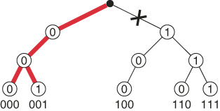
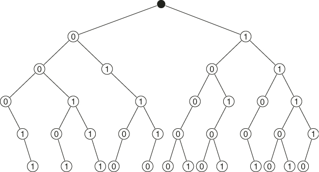
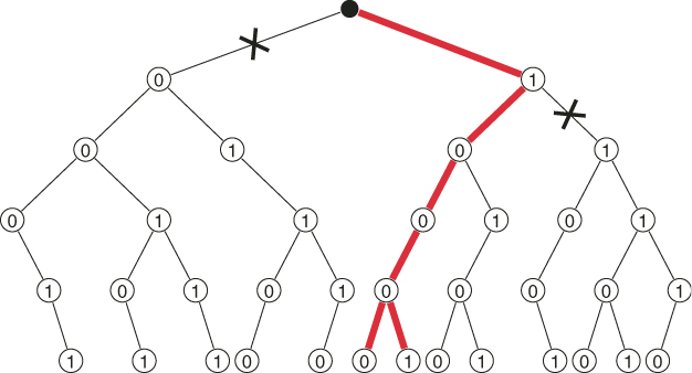
It follows from the above that by increasing ![]() from 1 to 2, the variance decreases 21 times. Figure 5.12 presents the subtrees
from 1 to 2, the variance decreases 21 times. Figure 5.12 presents the subtrees ![]() (in bold) of the original tree (based on the set
(in bold) of the original tree (based on the set ![]() ), generated using the oracle with
), generated using the oracle with ![]() .
.![]()
As mentioned earlier, the major advantage of SE Algorithm 5.3 versus its ![]() SLA counterpart is that the uniformity of
SLA counterpart is that the uniformity of ![]() in the former increases in
in the former increases in ![]() . In other words,
. In other words, ![]() becomes “closer” to the ideal pdf
becomes “closer” to the ideal pdf ![]() . We next demonstrate numerically this phenomenon while considering the following two simple models:
. We next demonstrate numerically this phenomenon while considering the following two simple models:
![]()
Table 5.2 The Efficiencies of the SE Algorithm 5.3 for the 2-SAT Model with ![]()
| RE | ||
| 11.110 | 0.296 | |
| 38.962 | 0.215 | |
| 69.854 | 0.175 | |
| 102.75 | 0.079 | |
| 101.11 | 0.032 | |
| 100.45 | 0.012 | |
| 100.00 | 0.000 |
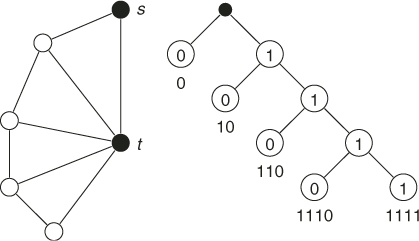
Figure 5.16 A ![]() graph and its associated tree with
graph and its associated tree with ![]() paths.
paths.
5.4 Applications of SE
Below we present several possible applications of SE. As usual we assume that there exists an associated polynomial time decision-making oracle.
5.4.1 Counting the Number of Trajectories in a Network
We show how to use SE for counting the number of trajectories (paths) in a network with a fixed source and sink. We demonstrate this for ![]() . The modification to
. The modification to ![]() is straightforward. Consider the following two toy examples.
is straightforward. Consider the following two toy examples.
between the source node ![]() and sink node
and sink node ![]() .
.
Note that if we select the combination ![]() instead of
instead of ![]() we would get again
we would get again ![]() and
and ![]() , and thus again an exact estimator
, and thus again an exact estimator ![]() .
.
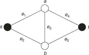
5.12 ![]()
then we obtain (with probability 1/2) an estimator ![]() for the path
for the path ![]() and (with probability 1/4) an estimator
and (with probability 1/4) an estimator ![]() for the paths
for the paths ![]() and
and ![]() , respectively.
, respectively.![]()
5.13 
| Path | Probability | Estimator |
| 8 | ||
| 8 | ||
| 8 | ||
| 8 | ||
| 6 | ||
| 6 | ||
| 6 |
Averaging over the all cases we obtain ![]() and thus, the exact value.
and thus, the exact value.![]()
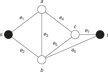
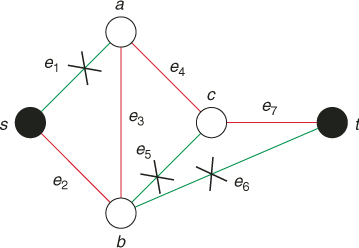
Consider now the case ![]() . In particular, consider the graph in Figure 5.18 and assume that
. In particular, consider the graph in Figure 5.18 and assume that ![]() . In this case, at iteration 1 of SE Algorithm 5.3 both edges
. In this case, at iteration 1 of SE Algorithm 5.3 both edges ![]() and
and ![]() will be selected. At iteration 2 we have to choose randomly two nodes out of the four:
will be selected. At iteration 2 we have to choose randomly two nodes out of the four: ![]() ,
, ![]() ,
, ![]() ,
, ![]() .Assume that
.Assume that ![]() and
and ![]() are selected. Note that by selecting
are selected. Note that by selecting ![]() , we completed an entire path,
, we completed an entire path, ![]() . Note, however, that the second path that goes through the edges
. Note, however, that the second path that goes through the edges ![]() ,
, ![]() will be not yet completed, since finally it can be either
will be not yet completed, since finally it can be either ![]() or
or ![]() . In both cases, the shorter path
. In both cases, the shorter path ![]() must be synchronized (length-wise) with the longer ones
must be synchronized (length-wise) with the longer ones ![]() or
or ![]() in the sense that, depending on whether
in the sense that, depending on whether ![]() or
or ![]() is selected, we have to insert into
is selected, we have to insert into ![]() either one auxiliary edge from
either one auxiliary edge from ![]() to
to ![]() (denoted
(denoted ![]() ) or two auxiliary ones from
) or two auxiliary ones from ![]() to
to ![]() (denoted by
(denoted by ![]() and
and ![]() ). The resulting path (with auxiliary edges) will be either
). The resulting path (with auxiliary edges) will be either ![]() or
or ![]() .
.
It follows from above that while adopting Algorithm 5.3 with ![]() for counting the number of paths in a general network, one will have to synchronize on-line all its paths with the longest one by adding some auxiliary edges until all paths will match length-wise with the longest one.
for counting the number of paths in a general network, one will have to synchronize on-line all its paths with the longest one by adding some auxiliary edges until all paths will match length-wise with the longest one.
5.4.2 SE for Probabilities Estimation
Algorithm 5.3 can be modified easily for the estimation of different probabilities in a network, such as the probability that the length ![]() of a randomly chosen path
of a randomly chosen path ![]() is greater than a fixed number
is greater than a fixed number ![]() , that is,
, that is,
![]()
Assume first that the length of each edge equals unity. Then the length ![]() of a particular path
of a particular path ![]() equals the number of edges from
equals the number of edges from ![]() to
to ![]() on that path. The corresponding number of iterations is
on that path. The corresponding number of iterations is ![]() and the corresponding probability is
and the corresponding probability is
![]()
Clearly, there is no need to calculate the weights ![]() and the length
and the length ![]() of each path
of each path ![]() .
.
In cases where the lengths of the edges are different from one, ![]() represents the sum of the lengths of edges associated with that path
represents the sum of the lengths of edges associated with that path ![]() .
.
- Full Enumeration. Same as in Algorithm 5.3.
- Calculation of the First Weight Factor. Redundant. Instead, store the lengths of the corresponding edges
 .
.
- Full Enumeration. Same as in Algorithm 5.3.
- Stochastic Enumeration. Same as in Algorithm 5.3.
- Calculation of the
 -th Weight Factor. Redundant. Instead, store the lengths of the corresponding edges
  .
.
- Proceed with iteration
 and compute
5.14
where, as before,
 is the length of path
  representing the sum of the lengths of the edges associated with
  .
.
- Run Algorithm 5.4 for
 independent replications and deliver
5.15 
We performed various numerical studies with Algorithm 5.4 and found that it performs properly, provided that ![]() is chosen such that
is chosen such that ![]() is not a rare-event probability; otherwise, one needs to use the importance sample method. For example, for a random Erdös-Rényi graph with 15 nodes and 50 edges (see Remark 5.3 below) we obtained via full enumeration that the number of valid paths is 643,085. Furthermore, the probability
is not a rare-event probability; otherwise, one needs to use the importance sample method. For example, for a random Erdös-Rényi graph with 15 nodes and 50 edges (see Remark 5.3 below) we obtained via full enumeration that the number of valid paths is 643,085. Furthermore, the probability ![]() that the length
that the length ![]() of a randomly chosen path
of a randomly chosen path ![]() is greater than
is greater than ![]() equals
equals ![]() . From our numerical results with
. From our numerical results with ![]() and
and ![]() based on 10 runs we obtained with Algorithm 5.4 an estimate
based on 10 runs we obtained with Algorithm 5.4 an estimate ![]() with relative error about 1%.
with relative error about 1%.
A simple way to generate a random graph in ![]() is to consider each of the possible
is to consider each of the possible ![]() edges in some order and then independently add each edge to the graph with probability
edges in some order and then independently add each edge to the graph with probability ![]() . Note that the expected number of edges in
. Note that the expected number of edges in ![]() is
is ![]() , and each vertex has expected degree
, and each vertex has expected degree ![]() . Clearly as
. Clearly as ![]() increases from 0 to 1, the model becomes more dense in the sense that is it is more likely that it will include graphs with more edges than less edges.
increases from 0 to 1, the model becomes more dense in the sense that is it is more likely that it will include graphs with more edges than less edges.
5.4.3 Counting the Number of Perfect Matchings in a Graph
Here we deal with application of SE to compute the number of matchings in a graph with particular emphasis on the number of perfect matchings in a balanced bipartite graph.
Recall that a graph ![]() is bipartite if it has no circuits of odd length. It has the following property: the set of vertices
is bipartite if it has no circuits of odd length. It has the following property: the set of vertices ![]() can be partitioned in two disjoint sets,
can be partitioned in two disjoint sets, ![]() and
and ![]() , such that each edge in
, such that each edge in ![]() has one vertex in
has one vertex in ![]() and one in
and one in ![]() . Thus, we denote a bipartite graph by
. Thus, we denote a bipartite graph by ![]() . In a balanced bipartite graph, the two subsets have the same cardinality:
. In a balanced bipartite graph, the two subsets have the same cardinality: ![]() . A matching of a graph
. A matching of a graph ![]() is a subset of the edges with the property that no two edges share the same node. In other words, a matching is a collection of edges
is a subset of the edges with the property that no two edges share the same node. In other words, a matching is a collection of edges ![]() such that each vertex occurs at most once in
such that each vertex occurs at most once in ![]() . A perfect matching is a matching that matches all vertices. Thus, a perfect matching in a balanced bipartite graph has size
. A perfect matching is a matching that matches all vertices. Thus, a perfect matching in a balanced bipartite graph has size ![]() .
.
Let ![]() be a balanced bipartite graph. Its associated biadjacency matrix
be a balanced bipartite graph. Its associated biadjacency matrix ![]() is an
is an ![]() binary matrix
binary matrix ![]() defined by
defined by
It is well known [90] that the number of perfect matchings in a balanced bipartite graph coincides with the permanent of its associated biadjacency matrix ![]() . The permanent of a binary
. The permanent of a binary ![]() matrix
matrix ![]() is defined as
is defined as
5.16 
where ![]() is the set of all permutations
is the set of all permutations ![]() of
of ![]() .
.
5.17 
Its associated biadjacency matrix is
5.18 
The permanent of ![]() is
is
![]()
We will show how SE works for ![]() . Its extension to
. Its extension to ![]() is simple. We say that an edge is active if the outcome of the corresponding variable is 1 and passive otherwise.
is simple. We say that an edge is active if the outcome of the corresponding variable is 1 and passive otherwise.
We next proceed separately with the outcomes ![]() and
and ![]() .
.
- Outcome (10)
a. Iteration 2 Recall that the outcome
 means that
  is active. This automatically implies that all three neighboring edges,
  ,
,  ,
,  , must be passive. Using the perfect matching oracle we will arrive at the next active edge, which is
  . Because the degree of node
  is two and since
  must be passive, we have that
  .b. Iteration 3 Because
 is active,
  must be passive. The degree of node
  is three, but since
  and
and  are passive,
  must be the only available active edge. This implies that
  . The resulting estimator of
  is
is 
- Outcome (01)
a. Iteration 2 Because (01) means that
 is active, we automatically set the neighboring edges
  ,
,  as passive. Using an oracle we shall arrive at node
  , which has degree three. As
  is passive, it is easily seen that each edge,
  and
and  , will become active with probability 1/2. This means that with
  and
and  we are in a similar situation (in the sense of active-passive edges) to that of
  , and
, and  . We thus have for each case
  .b. Iteration 3 It is readily seen that both cases
 , and
, and  lead to
  . The resulting estimator of
  is
is  . Because each initial edge
  and
and  at Iteration 1 is chosen with probability 1/2, by averaging over both cases we obtain the exact result, that is,
  .
.
![]()
The optimal zero variance importance sampling pdf is uniform on ![]() :
:
The SE procedure above with ![]() leads to an importance sampling pdf
leads to an importance sampling pdf ![]() satisfying
satisfying
The associated SE estimator satisfies
![]()
yielding ![]() , and
, and ![]() .
.![]()
5.4.4 Counting SAT
Note that, although for general SAT the decision-making is an NP-hard problem, there are several very fast heuristics for this purpose. The most popular one is the famous DPLL solver [35] (see Remark 5.19 below), on which two main heuristic algorithms are based for approximately counting with emphasis on SAT. The first, called ApproxCount and introduced by Wei and Selman in [126], is a local search method that uses Markov chain Monte Carlo sampling to approximate the true counting quantity. It is fast and has been shown to yield good estimates for feasible solution counts, but there are no guarantees as to uniformity of the Markov chain Monte Carlo samples. Gogate and Dechter [56] [57] recently proposed an alternative counting technique called SampleMinisat, based on sampling from the so-called backtrack-free search space of a Boolean formula through SampleSearch. An approximation of the search tree thus found is used as the importance sampling density instead of a uniform distribution over all solutions. They also derived a lower bound for the unknown counting quantity. Their empirical studies demonstrate the superiority of their method over its competitors.
5.5 Numerical Results
Here we present numerical results with the multiple-OSLA and SE algorithms. In particular, we use the multiple-OSLA Algorithm 5.2 for counting SAWs. The reason for doing so is that we are not aware of any polynomial decision-making algorithm (oracle) for SAWs. For the remaining problems we use the SE Algorithm 5.3 because polynomial decision-making algorithms (oracles) are available for them. If not stated otherwise, we use ![]() .
.
To achieve high efficiency of the SE Algorithm 5.3, we set ![]() as suggested in Section 5.3. In particular,
as suggested in Section 5.3. In particular,
We use the following notations:
5.5.1 Counting SAW
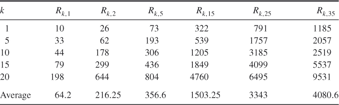
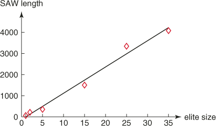
Tables 5.3 and 5.4 present the performance of the multiple-OSLA Algorithm 5.2 for SAW for ![]() and
and ![]() , respectively, with
, respectively, with ![]() ,
, ![]() , and
, and ![]() (see (5.8)). This corresponds to the initial values
(see (5.8)). This corresponds to the initial values ![]() and
and ![]() (see also iteration
(see also iteration ![]() in Table 5.5). Based on the runs in Table 5.3, we found
in Table 5.5). Based on the runs in Table 5.3, we found ![]() . Based on the runs in Table 5.4, we found
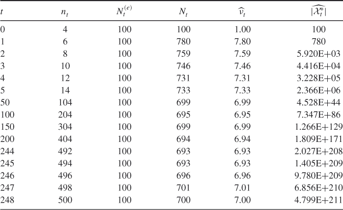
. Based on the runs in Table 5.4, we found ![]() . Table 5.5 presents dynamics of one of the runs of the multiple-OSLA Algorithm 5.2 for
. Table 5.5 presents dynamics of one of the runs of the multiple-OSLA Algorithm 5.2 for ![]() .
.
Table 5.3 Performance of the multiple-OSLA Algorithm 5.2 for counting SAW for ![]()
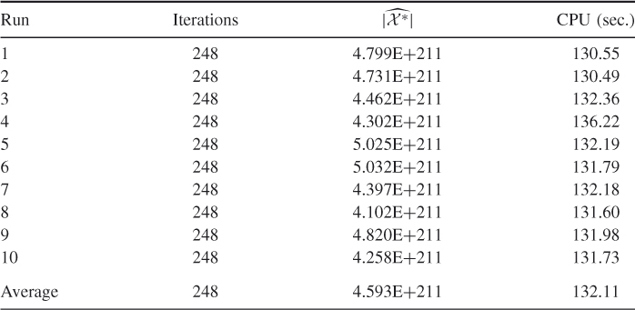
Table 5.4 Performance of the multiple-OSLA Algorithm 5.2 for counting SAW for ![]()
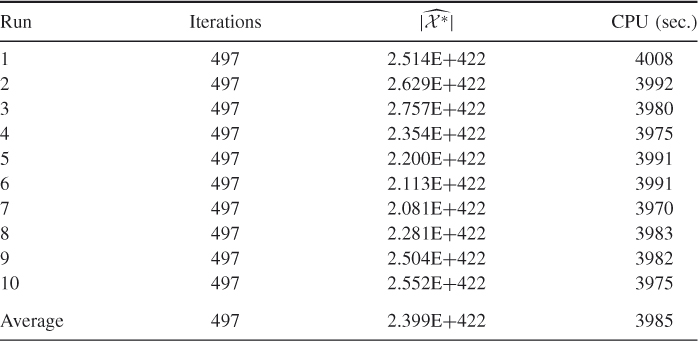
Table 5.5 Dynamics of a run of the multiple-OSLA Algorithm 5.2 for counting SAW for ![]()
5.5.2 Counting the Number of Trajectories in a Network
5.5.2.1 Model 1: From Roberts and Kroese [96] with  Nodes
Nodes
Table 5.6 presents the performance of the SE Algorithm 5.3 for Model 1 taken from Roberts and Kroese [96] with the following adjacency ![]() matrix:
matrix:
We set ![]() and
and ![]() to get a comparable running time.
to get a comparable running time.
Table 5.6 Performance of SE Algorithm 5.3 for counting trajectories in Model 1 Graph with ![]() and
and ![]()
Based on the runs in Table 5.6, we found ![]() . Comparing the results of Table 5.6 with those in [96], it follows that the former is about 1.5 times faster than the latter.
. Comparing the results of Table 5.6 with those in [96], it follows that the former is about 1.5 times faster than the latter.
5.5.2.2 Model 2: Large Model ( vertices and
  edges)
Table 5.7 presents the performance of SE Algorithm 5.3 for Model 2 with ![]() and
and ![]() . We found for this model
. We found for this model ![]() .
.
Table 5.7 Performance of SE Algorithm 5.3 for counting trajectories in Model 2 with ![]() and
and ![]()
We also counted the number of paths for Erdös-Rényi random graphs with ![]() (see Remark 5.3). We found that SE performs reliably (RE
(see Remark 5.3). We found that SE performs reliably (RE ![]() ) for
) for ![]() , provided the CPU time is limited to 5–15 minutes.
, provided the CPU time is limited to 5–15 minutes.
Table 5.8 presents the performance of SE Algorithm 5.3 for the Erdös-Rényi random graph with ![]() using
using ![]() and
and ![]() . We found
. We found ![]() .
.
Table 5.8 Performance of SE Algorithm 5.3 for counting trajectories in the Erdös-Rényi random graph ![]() with
with ![]() and
and ![]()
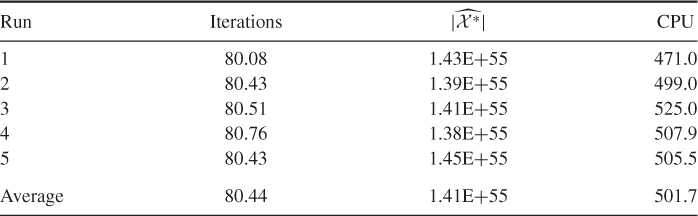
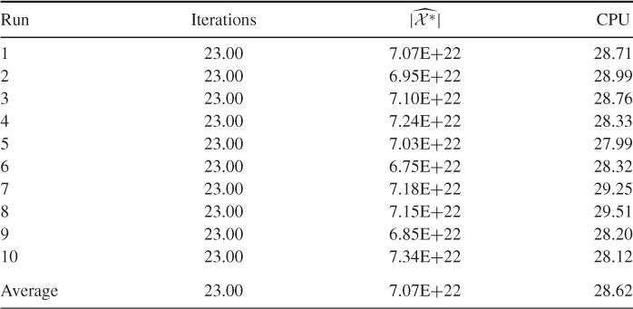
Table 5.9 presents the performance of SE Algorithm 5.3 for ![]() with
with ![]() and
and ![]() . The exact solution is 7.0273E+022. For this model we found
. The exact solution is 7.0273E+022. For this model we found ![]() , so the results are still good. However, as
, so the results are still good. However, as ![]() increases, the CPU time grows rapidly. For example, for
increases, the CPU time grows rapidly. For example, for ![]() we found that using
we found that using ![]() and
and ![]() the CPU time is about 5.1 hours.
the CPU time is about 5.1 hours.
5.5.3 Counting the Number of Perfect Matchings in a Graph
We present here numerical results for three models, one small and two large.
5.5.3.1 Model 1: (Small Model)
Consider the following ![]() matrix where the true number of perfect matchings (permanent) is
matrix where the true number of perfect matchings (permanent) is ![]() , obtained using full enumeration:
, obtained using full enumeration:
Table 5.10 presents the performance of SE Algorithm 5.3 for (![]() and
and ![]() ). We found that the relative error is
). We found that the relative error is ![]() .
.
Table 5.10 Performance of SE Algorithm 5.3 for counting perfect matchings in Model ![]() with
with ![]() and
and ![]()
Applying the splitting algorithm for the same model using ![]() and
and ![]() , we found that the relative error is 0.2711. It follows that SE is about 100 times faster than splitting.
, we found that the relative error is 0.2711. It follows that SE is about 100 times faster than splitting.
5.5.3.2 Model 2 with  (Large Model)
Table 5.11 presents the performance of SE Algorithm 5.3 for Model 2 matrix ![]() and
and ![]() . The relative error is 0.0434.
. The relative error is 0.0434.
Table 5.11 Performance of SE Algorithm 5.3 for counting perfect matchings in Model 2 with ![]() and
and ![]()
5.5.3.3 Model 3: Erdös-Rényi Graph with  Edges and
Table 5.12 presents the performance of SE Algorithm 5.3 for the Erdös-Rényi graph with ![]() edges and
edges and ![]() . We set
. We set ![]() and
and ![]() . We found that the relative error is 0.0387.
. We found that the relative error is 0.0387.
Table 5.12 Performance of SE Algorithm 5.3 for counting perfect matchings in the Erdös-Rényi random graph using ![]() and
and ![]()
We also applied the SE algorithm for counting general matchings in a bipartite graph. The quality of the results was similar to that for paths counting in a network.
5.5.4 Counting SAT
Here, we present numerical results for several SAT models. We set ![]() in the SE algorithm for all models. Recall that for 2-SAT we can use a polynomial decision-making oracle [35], whereas for
in the SE algorithm for all models. Recall that for 2-SAT we can use a polynomial decision-making oracle [35], whereas for ![]() -SAT
-SAT ![]() heuristic based on the DPLL solver [35] [36] is used. Note that SE Algorithm 5.3 remains exactly the same when a polynomial decision-making oracle is replaced by a heuristic one, such as the DPLL solver. Running both SAT models we found that the CPU time for 2-SAT is about 1.3 times faster than for
heuristic based on the DPLL solver [35] [36] is used. Note that SE Algorithm 5.3 remains exactly the same when a polynomial decision-making oracle is replaced by a heuristic one, such as the DPLL solver. Running both SAT models we found that the CPU time for 2-SAT is about 1.3 times faster than for ![]() -SAT
-SAT ![]() .
.
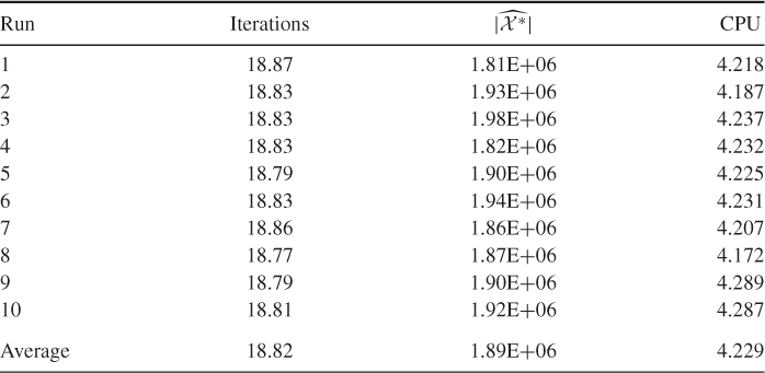
Table 5.13 presents the performance of SE Algorithm 5.3 for the 3-SAT ![]() model with exactly
model with exactly ![]() solutions. We set
solutions. We set ![]() and
and ![]() . Based on those runs, we found
. Based on those runs, we found ![]() .
.
Table 5.13 Performance of SE Algorithm 5.3 for the 3-SAT ![]() model
model
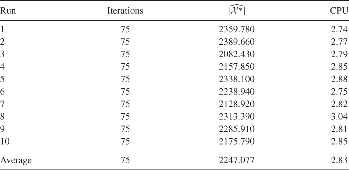
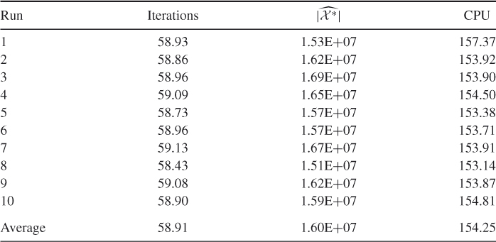
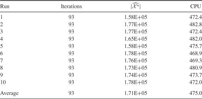
Table 5.14 presents the performance of SE Algorithm 5.3 for the 3-SAT ![]() model. We set
model. We set ![]() and
and ![]() . The exact solution for this instance is
. The exact solution for this instance is ![]() and is obtained via full enumeration using the backward method. It is interesting to note that, for this instance (with relatively small
and is obtained via full enumeration using the backward method. It is interesting to note that, for this instance (with relatively small ![]() ), the CPU time of the exact backward method is 332 seconds (compared with an average 16.8 seconds time of SE in Table 5.14). Based on those runs, we found that
), the CPU time of the exact backward method is 332 seconds (compared with an average 16.8 seconds time of SE in Table 5.14). Based on those runs, we found that ![]() .
.
Table 5.14 Performance of SE Algorithm 5.3 for the 3-SAT ![]() model
model
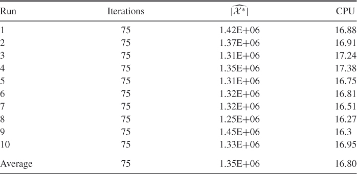
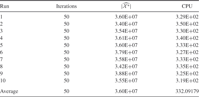
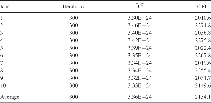
Table 5.15 presents the performance of SE Algorithm 5.3 for the 3-SAT ![]() model. We set
model. We set ![]() and
and ![]() . Based on those runs, we found
. Based on those runs, we found ![]() .
.
Table 5.15 Performance of SE Algorithm 5.3 for the 3-SAT ![]() model with
model with ![]() ,
, ![]() and
and ![]()
Note that, in this case, the estimator of ![]() is very large and, thus, full enumeration is impossible. We made, however, the exact solution
is very large and, thus, full enumeration is impossible. We made, however, the exact solution ![]() available as well. It is
available as well. It is ![]() 3.297E+24 and is obtained using a specially designed procedure (see Remark 5.6, below) for SAT instances generation. In particular, the instance matrix
3.297E+24 and is obtained using a specially designed procedure (see Remark 5.6, below) for SAT instances generation. In particular, the instance matrix ![]() was generated from the previous one
was generated from the previous one ![]() , for which
, for which ![]() .
.
of this instance. This solution consists of independent components of sizes ![]() , and it is straightforward to see that the total number of those solutions is
, and it is straightforward to see that the total number of those solutions is ![]() . It follows, therefore, that one can easily construct a large SAT instance from a set of small ones and still have an exact solution for it. Note that the above
. It follows, therefore, that one can easily construct a large SAT instance from a set of small ones and still have an exact solution for it. Note that the above ![]() instance with exactly
instance with exactly ![]() solutions was obtained from the four identical instances of size
solutions was obtained from the four identical instances of size ![]() , each with exactly 1,346,963 solutions.
, each with exactly 1,346,963 solutions.
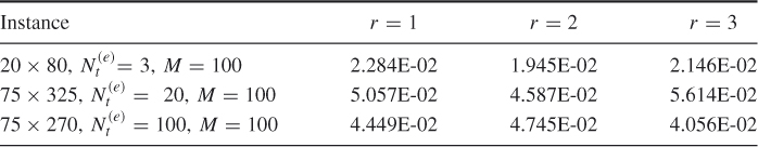
We also performed experiments with different values of ![]() . Table 5.16 summarizes the results. In particular, it presents the relative error for
. Table 5.16 summarizes the results. In particular, it presents the relative error for ![]() , and
, and ![]() with SE run for a predefined time period foreach instance. We can see that changing
with SE run for a predefined time period foreach instance. We can see that changing ![]() does not affect the relative error.
does not affect the relative error.
Table 5.16 The relative errors as functions of ![]()
5.5.5 Comparison of SE with Splitting and SampleSearch
Here we compare SE with splitting and SampleSearch for several 3-SAT instances. Before doing so we require the following remarks.
5.19 ![]()
Table 5.17 presents a comparison of the efficiencies of SE (at ![]() ) with those of SampleSearch and splitting (SaS and Split columns, respectively) for several SAT instances. We ran all three methods for the same amount of time.
) with those of SampleSearch and splitting (SaS and Split columns, respectively) for several SAT instances. We ran all three methods for the same amount of time.
Table 5.17 Comparison of the efficiencies of SE, SampleSearch and standard splitting
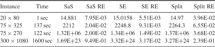
In terms of speed (which equals (RE)![]() ), SE is faster than SampleSearch by about 2–10 times and standard splitting in [104] by about 20–50 times. Similar comparison results were obtained for other models, including perfect matching. Our explanation is that SE is an SIS method, whereas SampleSearch and splitting are not, in the sense that SE samples sequentially with respect to coordinates
), SE is faster than SampleSearch by about 2–10 times and standard splitting in [104] by about 20–50 times. Similar comparison results were obtained for other models, including perfect matching. Our explanation is that SE is an SIS method, whereas SampleSearch and splitting are not, in the sense that SE samples sequentially with respect to coordinates ![]() , whereas the other two sample (random vectors
, whereas the other two sample (random vectors ![]() from the IS pdf
from the IS pdf ![]() ) in the entire
) in the entire ![]() -dimensional space.
-dimensional space.