
Chapter 4
Splitting Method for Counting and Optimization
4.1 Background
This chapter deals with the splitting method for counting, combinatorial optimization, and rare-event estimation. Before turning to the splitting method we present some background on counting using randomized (or Monte Carlo) algorithms.
To date, very little is known about how to construct efficient algorithms for hard counting problems. This means that exact solutions to these problems cannot be obtained in polynomial time, and therefore our work focuses on approximation algorithms, and, in particular, approximation algorithms based on randomization. The basic procedure for counting is outlined below.
and ![]() is known.
is known.
where
Using (4.1)(4.2)(4.3)(4.4)(4.5), one can design a sampling plan according to which the “difficult” counting problem defined on the set ![]() is decomposed into a number of “easy” ones associated with a sequence of related sets
is decomposed into a number of “easy” ones associated with a sequence of related sets ![]() and such that
and such that ![]() . Typically, the Monte Carlo algorithms based on (4.1)(4.2)(4.3)(4.4)(4.5) explore the connection between counting and sampling and in particular the reduction from approximate counting of a discrete set to approximate sampling of the elements of this set [108].
. Typically, the Monte Carlo algorithms based on (4.1)(4.2)(4.3)(4.4)(4.5) explore the connection between counting and sampling and in particular the reduction from approximate counting of a discrete set to approximate sampling of the elements of this set [108].
To deliver a meaningful estimator of ![]() , we must solve the following two major problems:
, we must solve the following two major problems:
Hence, once both tasks (i) and (ii) are resolved, one can obtain an efficient estimator for ![]() given in (4.5).
given in (4.5).
Task (i) might be typically simply resolved in many cases. Let us consider a concrete example:
- Suppose that each variable of the set (1.1) is bounded, say

 (
( ), then we may take
  , with
  .
. - Consider the function
 to be the number of constraints of the integer program (1.1); hence,
  .
. - Define finally the desired subregions
 by
by

Task (ii) is quite complicated. It is associated with uniform sampling separately at each subregion ![]() and will be addressed in the subsequent text.
and will be addressed in the subsequent text.
The rest of this chapter is organized as follows. Section 4.2 presents a quick look at the splitting method. We show that, similarly to the conventional classic randomized algorithms (see [88]), it uses a sequential sampling plan to decompose a “difficult” problem into a sequence of “easy” ones. Sections 4.3 and 4.4 present two different splitting algorithms for counting; the first based on a fixed-level set and the second on an adaptive level set. Both algorithms employ a combination of a Markov chain Monte Carlo algorithm, such as the Gibbs sampler, with a specially designed cloning mechanism. The latter runs in parallel multiple Markov chains by making sure that all of them run in steady-state at each iteration. Section 4.5 shows how, using the splitting method, one can generate a sequence of points ![]() uniformly distributed on a discrete set
uniformly distributed on a discrete set ![]() . By uniformity we mean that the sample
. By uniformity we mean that the sample ![]() on
on ![]() passes the standard Chi-squared test [91]. We support numerically the uniformity of generated samples based on the Chi-squared test.
passes the standard Chi-squared test [91]. We support numerically the uniformity of generated samples based on the Chi-squared test.
In Section 4.6 we show that the splitting method is suitable for solving combinatorial optimization problems, such as the maximal cut or traveling salesman problems, and thus can be considered as an alternative to the standard cross-entropy and MinxEnt methods. Sections 4.7.1 and 4.7.2 deal with two enhancements of theadaptive splitting method for counting. The first is called the direct splitting estimator and is based on the direct counting of ![]() , while the second is called the capture-recapture estimator of
, while the second is called the capture-recapture estimator of ![]() . It has its origin in the well-known capture-recapture method in statistics [114]. Both are used to obtain low-variance estimators for counting on complex sets as compared to the adaptive splitting algorithm. Section 4.8 shows how the splitting algorithm can be efficiently used for estimating the reliability of complex static networks. Finally, Section 4.9 presents supportive numerical results for counting, rare events, and optimization.
. It has its origin in the well-known capture-recapture method in statistics [114]. Both are used to obtain low-variance estimators for counting on complex sets as compared to the adaptive splitting algorithm. Section 4.8 shows how the splitting algorithm can be efficiently used for estimating the reliability of complex static networks. Finally, Section 4.9 presents supportive numerical results for counting, rare events, and optimization.
4.2 Quick Glance at the Splitting Method
In this section we will take a quick look at our sampling mechanism using splitting. Consider the counting problem (4.2) with ![]() subsets, that is,
subsets, that is,
where ![]() . We assume that the subsets
. We assume that the subsets ![]() are associated with levels
are associated with levels ![]() and can be written as
and can be written as
![]()
where ![]() is the sample performance function and
is the sample performance function and ![]() . We set for convenience
. We set for convenience ![]() . The other levels are either fixed in advance, or their values are determined adaptively by the splitting algorithm during the course of simulation. Observe that
. The other levels are either fixed in advance, or their values are determined adaptively by the splitting algorithm during the course of simulation. Observe that ![]() in (4.3) can be interpreted as
in (4.3) can be interpreted as
where ![]() , the uniform distribution on
, the uniform distribution on ![]() . We denote this by
. We denote this by ![]() . Furthermore, we shall require a uniform pdf on each subset
. Furthermore, we shall require a uniform pdf on each subset ![]() , which is denoted by
, which is denoted by ![]() .Clearly,
.Clearly,
where ![]() is the normalization constant. Generating points uniformly distributed on
is the normalization constant. Generating points uniformly distributed on ![]() using the splitting method will be addressed in Section 4.5. With these notations, we can consider
using the splitting method will be addressed in Section 4.5. With these notations, we can consider ![]() of (4.4) to be a conditional expectation defined as
of (4.4) to be a conditional expectation defined as
Suppose that sampling from ![]() becomes available, and that we generated
becomes available, and that we generated ![]() samples in
samples in ![]() , then the final estimators of
, then the final estimators of ![]() and
and ![]() can be written as
can be written as
and
respectively. Here we used
as estimators of their true unknown conditional expectations. Furthermore, ![]() , with
, with ![]() and
and ![]() . We call
. We call ![]() the elite sample size, associated with the elite samples.
the elite sample size, associated with the elite samples.
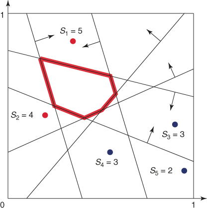
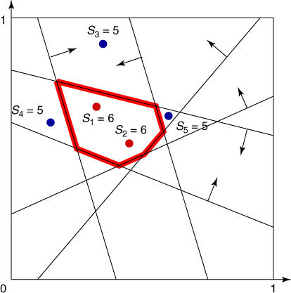
To provide more insight into the splitting method, consider a toy example of the integer problem (1.1), pictured in Figure 4.1. The solution set is a six-sided polytope in the two-dimensional plane, obtained by ![]() inequality constraints. Its boundary is shown by the bold lines in the figure. The bounding set is the unit square
inequality constraints. Its boundary is shown by the bold lines in the figure. The bounding set is the unit square ![]() . We generate
. We generate ![]() points uniformly in
points uniformly in ![]() (see the dots in the figure). The corresponding five performance values
(see the dots in the figure). The corresponding five performance values ![]() ,
, ![]() are
are
![]()
Figure 4.1 Iteration 1: five uniform samples on ![]() .
.
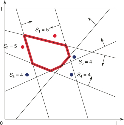
As for elite samples, we choose the two largest values corresponding to ![]() and
and ![]() . We thus have
. We thus have ![]() , and
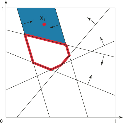
, and ![]() . Consider the first elite sample
. Consider the first elite sample ![]() with
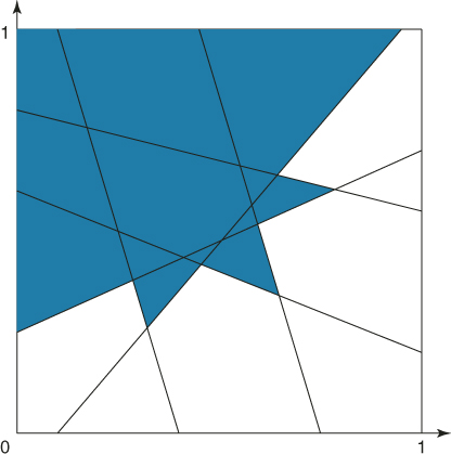
with ![]() . Its associated subregion of points satisfying exactly the same five constraints is given by the shaded area in Figure 4.2.
. Its associated subregion of points satisfying exactly the same five constraints is given by the shaded area in Figure 4.2.
Figure 4.2 The subregion corresponding to the elite point ![]() with
with ![]() .
.
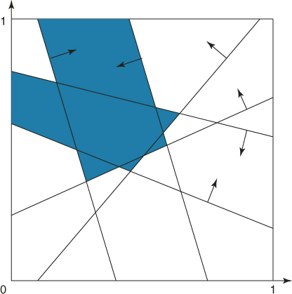
Similarly, Figure 4.3 shows the elite point ![]() (with
(with ![]() ) and its associated subregion of points satisfying the same four constraints. However, notice that there are more subregions of points satisfying at least four constraints. The union of all these subregions is the set
) and its associated subregion of points satisfying the same four constraints. However, notice that there are more subregions of points satisfying at least four constraints. The union of all these subregions is the set ![]() ; that is,
; that is,
![]()
as shown in Figure 4.4.
Figure 4.3 The subregion corresponding to the elite point ![]() with
with ![]() .
.
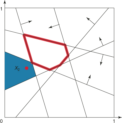
Figure 4.4 The subregion ![]() containing all points with
containing all points with ![]() .
.
Starting from the two elite points ![]() , we apply a Markov chain Monte Carlo algorithm that generates points in
, we apply a Markov chain Monte Carlo algorithm that generates points in ![]() such that these points are uniformly distributed. Figure 4.5 shows
such that these points are uniformly distributed. Figure 4.5 shows ![]() resulting points. The five performance values are
resulting points. The five performance values are
Figure 4.5 Iteration 2: five uniform points on ![]() .
.
![]()
Next, we repeat the same procedure as in the first iteration. As elite samples we choose the two largest points ![]() . Thus,
. Thus, ![]() , and
, and ![]() . This gives us the set of all points satisfying at least five constraints,
. This gives us the set of all points satisfying at least five constraints,
![]()
see Figure 4.6.
Figure 4.6 The subregion ![]() containing all points with
containing all points with ![]() .
.
We use a Markov chain Monte Carlo algorithm to generate from the two elite points five new points in ![]() , uniformly distributed; see Figure 4.7. Note that two of the new points hit the desired polytope. At this stage, we stop the iterations and conclude that the algorithm has converged. The purpose of Figures 4.1–4.7 is to demonstrate that the splitting method can be viewed as a global search in the sense that, at each iteration, the generated random points
, uniformly distributed; see Figure 4.7. Note that two of the new points hit the desired polytope. At this stage, we stop the iterations and conclude that the algorithm has converged. The purpose of Figures 4.1–4.7 is to demonstrate that the splitting method can be viewed as a global search in the sense that, at each iteration, the generated random points ![]() are randomly distributed inside their corresponding subregion. The main issue remaining in the forthcoming sections is to provide exact algorithms that implement the splitting method.
are randomly distributed inside their corresponding subregion. The main issue remaining in the forthcoming sections is to provide exact algorithms that implement the splitting method.
Figure 4.7 Iteration 3: five uniform points on ![]() .
.
Before doing so, we show how to cast the problem of counting the number of what we call multiple events into the framework (4.6)–(4.8). As we shall see below, counting the number of feasible points ![]() of the set (1.1) follows as a particular case of it.
of the set (1.1) follows as a particular case of it.
where ![]() are arbitrary functions. In this case, we can associate with (4.12) the following multiple-event probability estimation problem:
are arbitrary functions. In this case, we can associate with (4.12) the following multiple-event probability estimation problem:
Note that (4.13) extends (4.6) in the sense that it involves an intersection of ![]() events
events ![]() , that is, multiple events rather than a single one
, that is, multiple events rather than a single one ![]() . Some of the constraints may be equality constraints,
. Some of the constraints may be equality constraints, ![]() .
.
where
4.15 ![]()
For the cardinality of the set ![]() one applies (4.10), which means that one only needs to estimate the rare-event probability
one applies (4.10), which means that one only needs to estimate the rare-event probability ![]() in (4.14) according to (4.9).
in (4.14) according to (4.9).![]()
4.3 Splitting Algorithm with Fixed Levels
In this section we assume that the levels ![]() are fixed in advance, with
are fixed in advance, with ![]() . This can be done using a pilot run with the splitting method as in [73]. Consider the problem of estimating the conditional probability
. This can be done using a pilot run with the splitting method as in [73]. Consider the problem of estimating the conditional probability
![]()
Assume further that we have generated a point ![]() uniformly distributed on
uniformly distributed on ![]() , that is,
, that is, ![]() . Recall from our toy example in the previous section that, given this information of the current point, we should be able to generate a new point in
. Recall from our toy example in the previous section that, given this information of the current point, we should be able to generate a new point in ![]() , which is again uniformly distributed. Typically, this might be obtained by applying a Markov chain Monte Carlo technique. For now we just assume that we dispose of a mapping
, which is again uniformly distributed. Typically, this might be obtained by applying a Markov chain Monte Carlo technique. For now we just assume that we dispose of a mapping ![]() , which preserves uniformity, that is,
, which preserves uniformity, that is,
4.16 ![]()
We call this mapping the uniform mutation mapping. Based on that we can derive an unbiased estimator of ![]() by using the followingprocedure:
by using the followingprocedure:
The following algorithm applies this procedure iteratively. Moreover, in each iteration all ![]() elite points are reproduced (cloned)
elite points are reproduced (cloned) ![]() times to form a new sample of
times to form a new sample of ![]() points. The parameter
points. The parameter ![]() is called the splitting parameter.
is called the splitting parameter.
- Input: the counting problem (1.1); the fixed levels
 ;
;  ;
;  ; the splitting parameters
  ; the initial sample size
  .
. - Output: estimators (4.9) and (4.10).
![]()
A key ingredient in the Algorithm 4.1 is the uniform mutation mapping ![]() . Typically, this is obtained by a Markov chain kernel
. Typically, this is obtained by a Markov chain kernel ![]() on
on ![]() with the uniform distribution as its invariant distribution. This means that we assume:
with the uniform distribution as its invariant distribution. This means that we assume:
![]()
for measurable subsets ![]() .
.
![]()
Under these assumptions, we can generate from any point ![]() a path of points
a path of points ![]() in
in ![]() , by repeatedly applying the Markov kernel
, by repeatedly applying the Markov kernel ![]() . If the initial point is random uniformly distributed, then each consecutive point of the path preserves this property (assumption (iii)). Otherwise, we use the property that the limiting distribution of Markov chain is its invariant distribution. In implementations we often resort to the Gibbs sampler for constructing the Markov kernel and generating an associated path of points (see Appendix 4.10 for details). All these considerations are summarized in just mentioning “apply the uniform mutation mapping.”
. If the initial point is random uniformly distributed, then each consecutive point of the path preserves this property (assumption (iii)). Otherwise, we use the property that the limiting distribution of Markov chain is its invariant distribution. In implementations we often resort to the Gibbs sampler for constructing the Markov kernel and generating an associated path of points (see Appendix 4.10 for details). All these considerations are summarized in just mentioning “apply the uniform mutation mapping.”
We next show that the estimator ![]() is unbiased. Indeed taking into account that
is unbiased. Indeed taking into account that
we obtain from the last two equalities that
from which ![]() readily follows. We next calculate the variance of
readily follows. We next calculate the variance of ![]() . In order to accomplish this, we do the following:
. In order to accomplish this, we do the following:
4.17 ![]()
where
![]()
and
![]()
Thus, to estimate the variance of ![]() it suffices to estimate
it suffices to estimate ![]() , which in turn can be calculated as
, which in turn can be calculated as
where
and ![]() are iid samples.
are iid samples.
It is challenging to find good splitting parameters ![]() in the fixed-level splitting version. When these parameters are not chosen correctly, the number of samples will either die out or explode, leading in both cases to large variances of
in the fixed-level splitting version. When these parameters are not chosen correctly, the number of samples will either die out or explode, leading in both cases to large variances of ![]() . The minimal variance choice is
. The minimal variance choice is ![]() , see [48] and [55]. Thus, given the levels
, see [48] and [55]. Thus, given the levels ![]() , we can execute pilot runs to find rough estimates of the
, we can execute pilot runs to find rough estimates of the ![]() 's, denoted by
's, denoted by ![]() . At iteration
. At iteration ![]() (
(![]() ) of the algorithm we set the splitting parameter of the
) of the algorithm we set the splitting parameter of the ![]() -th elite point to be a random variable defined as
-th elite point to be a random variable defined as
![]()
where the variable ![]() is a Bernoulli random variable with success probability
is a Bernoulli random variable with success probability ![]() , and
, and ![]() means rounding down to the nearest integer. Thus, the splitting parameters satisfy
means rounding down to the nearest integer. Thus, the splitting parameters satisfy ![]() . Note that the sample size in the next iteration is also a random variable defined as
. Note that the sample size in the next iteration is also a random variable defined as
In the following section we propose an adaptive splitting method considering two issues that can cause difficulties in the fixed-level approach:
- An objection against cloning is that it introduces correlation. An alternative approach is to sample
 “new” points in the current subset by running a Markov chain using a Markov chain Monte Carlo method.
 - Finding “good” locations of the levels
 is crucial but difficult. We propose to select the levels adaptively.
4.4 Adaptive Splitting Algorithm
In both counting and optimization problems the proposed adaptive splitting algorithms generate sequences of pairs
4.18 ![]()
where, as before, ![]() . This is in contrast to the cross-entropy method [107], where one generates a sequence of pairs
. This is in contrast to the cross-entropy method [107], where one generates a sequence of pairs
4.19 ![]()
Here ![]() is a sequence of parameters in the parametric family of distributions
is a sequence of parameters in the parametric family of distributions ![]() . The crucial difference is, of course, that in the splitting method,
. The crucial difference is, of course, that in the splitting method, ![]() is a sequence of (uniform) nonparametric distributions rather than of parametric ones
is a sequence of (uniform) nonparametric distributions rather than of parametric ones ![]() . Otherwise the cross-entropy and the splitting algorithms are very similar, apart from the fact that cross-entropy has the desirable property that the samples are independent, whereas in splitting they are not. The advantage of the splitting method is that it permits approximate sampling from the uniform pdf
. Otherwise the cross-entropy and the splitting algorithms are very similar, apart from the fact that cross-entropy has the desirable property that the samples are independent, whereas in splitting they are not. The advantage of the splitting method is that it permits approximate sampling from the uniform pdf ![]() and permits updating the parameters
and permits updating the parameters ![]() and
and ![]() adaptively. It is shown in [104] that for rare-event estimation and counting the splitting method typically outperforms its cross-entropy counterpart, while for combinatorial optimization they perform similarly. The main reason is that for counting the sampling from a sequence of nonparametric probability density function
adaptively. It is shown in [104] that for rare-event estimation and counting the splitting method typically outperforms its cross-entropy counterpart, while for combinatorial optimization they perform similarly. The main reason is that for counting the sampling from a sequence of nonparametric probability density function ![]() is more beneficial (more informative) than sampling from a sequence of a parametric family like
is more beneficial (more informative) than sampling from a sequence of a parametric family like ![]() .
.
Below we present the main steps of the adaptive splitting algorithm. However, first, we describe the main ideas for which we refer to [13] and [40], where the adaptive ![]() -thresholds satisfy the requirements
-thresholds satisfy the requirements ![]() . Here, as before, the parameters
. Here, as before, the parameters ![]() , called the rarity parameters, are fixed in advance and they must be not too small, say
, called the rarity parameters, are fixed in advance and they must be not too small, say ![]() .
.
We start by generating a sample of ![]() points uniformly on
points uniformly on ![]() , denoted by
, denoted by ![]() . Consider the sample set at the
. Consider the sample set at the ![]() -th iteration:
-th iteration: ![]() of
of ![]() random points in
random points in ![]() . All these sampled points are uniformly distributed on
. All these sampled points are uniformly distributed on ![]() . Let
. Let ![]() be the
be the ![]() -th quantile of the ordered statistics values of the values
-th quantile of the ordered statistics values of the values ![]() . The elite set
. The elite set ![]() consists of those points of the sample set for which
consists of those points of the sample set for which ![]() . Let
. Let ![]() be the size of the elite set. If all values
be the size of the elite set. If all values ![]() would be distinct, it would follow that the number of elites
would be distinct, it would follow that the number of elites ![]() , where
, where ![]() denotes rounding up to the nearest integer. However, when we deal with a discrete finite space, typically we will find many duplicate sampled pointswith
denotes rounding up to the nearest integer. However, when we deal with a discrete finite space, typically we will find many duplicate sampled pointswith ![]() . All these are included in the elite set. Level
. All these are included in the elite set. Level ![]() is used to define the next level subset
is used to define the next level subset ![]() . Finally, note that it easily follows from (4.7) that the elite points are distributed uniformly on this level subset.
. Finally, note that it easily follows from (4.7) that the elite points are distributed uniformly on this level subset.
Regarding the elite sample ![]() , we do three things. First, we use its relative size
, we do three things. First, we use its relative size ![]() as an estimate of the conditional probability
as an estimate of the conditional probability ![]() . Next, we delete duplicates. We call this screening, and it might be modeled formally by introducing the identity map
. Next, we delete duplicates. We call this screening, and it might be modeled formally by introducing the identity map ![]() ; that is,
; that is, ![]() for all points
for all points ![]() . Apply the identity map
. Apply the identity map ![]() to the elite set, resulting in a set of
to the elite set, resulting in a set of ![]() distinct points (called the screened elites), that we denote by
distinct points (called the screened elites), that we denote by
4.20 ![]()
Thirdly, each screened elite is the starting point of ![]() trajectories in
trajectories in ![]() generated by a Markov chain simulation using a transition probability matrix with
generated by a Markov chain simulation using a transition probability matrix with ![]() as its stationary distribution. Because the starting point is uniformly distributed, all consecutive points on the sample paths are uniformly distributed on
as its stationary distribution. Because the starting point is uniformly distributed, all consecutive points on the sample paths are uniformly distributed on ![]() . Therefore, we may use all these points in the next iteration. If the splitting parameter
. Therefore, we may use all these points in the next iteration. If the splitting parameter ![]() , all trajectories are independent.
, all trajectories are independent.
Thus, we simulate ![]() trajectories, each trajectory for
trajectories, each trajectory for ![]() steps. This produces a total of
steps. This produces a total of ![]() uniform points in
uniform points in ![]() . To continue with the next iteration again with a sample set of size
. To continue with the next iteration again with a sample set of size ![]() , we choose randomly
, we choose randomly ![]() of the generated trajectories (without replacement) and apply one more Markov chain transition to the end points of these trajectories. Denote the new sample set by
of the generated trajectories (without replacement) and apply one more Markov chain transition to the end points of these trajectories. Denote the new sample set by ![]() , and repeat the same procedure as above. Summarizing the above:
, and repeat the same procedure as above. Summarizing the above:
4.21 
The algorithm iterates until it converges to ![]() , say at iteration
, say at iteration ![]() , at which stage we stop and deliver the estimators (4.9) and (4.10) of
, at which stage we stop and deliver the estimators (4.9) and (4.10) of ![]() and
and ![]() , respectively.
, respectively.
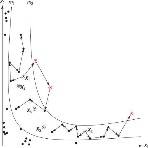
Figure 4.8 represents a typical dynamics of the zero-th iteration of the adaptive splitting algorithm below for counting. Initially ![]() points were generated randomly in the two-dimensional space
points were generated randomly in the two-dimensional space ![]() (some are shown as black dots). Because
(some are shown as black dots). Because ![]() , the elite sample consists of
, the elite sample consists of ![]() points (shown as the
points (shown as the ![]() points numbered
points numbered ![]() ) with values
) with values ![]() . After renumbering, these five points are
. After renumbering, these five points are ![]() . From each of these elite points
. From each of these elite points ![]() Markov chain paths of length
Markov chain paths of length ![]() were generated resulting in again
were generated resulting in again ![]() points in the space
points in the space ![]() . In the picture we see these paths from two points
. In the picture we see these paths from two points ![]() and
and ![]() . Three points (the
. Three points (the ![]() in the upper region) are shown reaching the next-level
in the upper region) are shown reaching the next-level ![]() .
.
- Input: The counting problem (4.2); the rarity parameters
 ; the splitting parameters
  ; the sample size
  .
. - Output: Estimators (4.9) and (4.10).
![]()
Figure 4.8 Iteration of the splitting algorithm.
As an illustrative example, one may consider a sum of Bernoulli random variables. Suppose we have ![]() for
for ![]() and we are interested in calculating a probability of the event
and we are interested in calculating a probability of the event ![]() for fixed
for fixed ![]() ,
, ![]() . One should note that even for moderate
. One should note that even for moderate ![]() and, say,
and, say, ![]() we have a rare-event scenario. Let now
we have a rare-event scenario. Let now ![]() be the performance function. The Gibbs sampler can be defined as follows:
be the performance function. The Gibbs sampler can be defined as follows:
- Input: A random Bernoulli vector
 where
where 
- Output: A uniformly chosen random neighbor
 with the same property.
For each ![]() do:
do:
From this simple example, it is clear that if we repeatedly apply this algorithm on any vector ![]() , it will eventually approach the desired event space
, it will eventually approach the desired event space ![]()
![]() .
.
We conclude with a few remarks.
- Include in the elite sample all additional points satisfying
 , provided that the number of elite samples
  .
. -
Remove from the elite sample all points
 , provided the number of elite samples
  . Note that by doing so we switch from a lower elite level to a higher one. If
  , and thus
  , accept
  as the size of the elites sample. If
  , proceed sampling until
  , that is until at least
  elite samples are obtained. The above guarantees that
  .It follows that such adaptive
 satisfying
  prevents Algorithm 4.2 of being stopped before reaching the target level
  .
.
4.5 Sampling Uniformly on Discrete Regions
Here we demonstrate how, using the splitting method, one can generate a sequence of points ![]() nearly uniformly distributed on a discrete set
nearly uniformly distributed on a discrete set ![]() , such as the set (1.1). By near uniformity we mean that the sample
, such as the set (1.1). By near uniformity we mean that the sample ![]() on
on ![]() passes the standard Chi-square test. Thus, the goal of Algorithm 4.2 is twofold: counting the points on the set
passes the standard Chi-square test. Thus, the goal of Algorithm 4.2 is twofold: counting the points on the set ![]() and simultaneously generating points uniformly distributed on that set
and simultaneously generating points uniformly distributed on that set ![]() .
.
Note that generating a sample of points uniformly distributed on a continuous set ![]() using a Markov chain Monte Carlo algorithm has been thoroughly studied in the literature. One of the most popular methods is the hit-and-run of Smith [53]. For recent applications of hit-and-run for convex optimization, see the work of Gryazina and Polyak [58].
using a Markov chain Monte Carlo algorithm has been thoroughly studied in the literature. One of the most popular methods is the hit-and-run of Smith [53]. For recent applications of hit-and-run for convex optimization, see the work of Gryazina and Polyak [58].
We will show empirically that a simple modification of the splitting Algorithm 4.2 allows one to generate points uniformly distributed on sets like (1.1). The modification of the Algorithm 4.2 is very simple. Once it reaches the desired level ![]() we perform several more iterations, say
we perform several more iterations, say ![]() iterations, with the corresponding elite samples. As for previous iterations, we use here the screening, splitting, and sampling steps. Such policy will only improve the uniformity of the samples on
iterations, with the corresponding elite samples. As for previous iterations, we use here the screening, splitting, and sampling steps. Such policy will only improve the uniformity of the samples on ![]() . The number of additional steps
. The number of additional steps ![]() needed for the resulting sample to pass the Chi-square test for uniformity, depends on the quality of the original elite sample at level
needed for the resulting sample to pass the Chi-square test for uniformity, depends on the quality of the original elite sample at level ![]() , which in turn depends on the selected values
, which in turn depends on the selected values ![]() and
and ![]() . We found numerically that the closer
. We found numerically that the closer ![]() is to 1, the more uniform is the sample. But, running the splitting Algorithm 4.2 at
is to 1, the more uniform is the sample. But, running the splitting Algorithm 4.2 at ![]() close to 1 is clearly time consuming. Thus, there exists a trade-off between the quality (uniformity) of the sample and the number of additional iterations
close to 1 is clearly time consuming. Thus, there exists a trade-off between the quality (uniformity) of the sample and the number of additional iterations ![]() required.
required.
As an example, consider a ![]() -SAT problem consisting of
-SAT problem consisting of ![]() literals and
literals and ![]() clauses and
clauses and ![]() (see also Section 4.9 with the numerical results). We applied the Chi-square test for uniformity of
(see also Section 4.9 with the numerical results). We applied the Chi-square test for uniformity of ![]() samples for the following cases:
samples for the following cases:
 and no additional iterations (
 );
); and no additional iterations (
 );
); and one additional iteration (
 ).
).
All three experiments passed the Chi-square test at level ![]() : the observed test values were 13.709, 9.016, and 8.434, respectively, against critical value
: the observed test values were 13.709, 9.016, and 8.434, respectively, against critical value ![]() . The histogram corresponding to the last experiment (
. The histogram corresponding to the last experiment (![]() ) is shown in Figure 4.10.
) is shown in Figure 4.10.
Figure 4.10 Histogram of 5,000 samples for the 3-SAT problem.
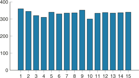
In this way, we tested many more SAT problems for uniformity and found that typically (about 95%) the resulting samples pass the Chi-square test, provided we perform two or three additional iterations (![]() ) on the corresponding elite sample after the algorithm has reached the desired level
) on the corresponding elite sample after the algorithm has reached the desired level ![]() .
.
4.6 Splitting Algorithm for Combinatorial Optimization
In this section, we show that the splitting method is suitable for solving combinatorial optimization problems, such as the maximum cut or traveling salesman problems, and, thus, can be considered as an alternative to the standard cross-entropy and MinxEnt methods. The splitting algorithm for combinatorial optimization can be considered as a particular case of the counting Algorithm 4.2 with ![]() . In that case, we do not need to calculate the product estimators
. In that case, we do not need to calculate the product estimators ![]() ; thus, Step 3 of Algorithm 4.2 is omitted. The main difference reflects the stopping step.
; thus, Step 3 of Algorithm 4.2 is omitted. The main difference reflects the stopping step.
4.22 ![]()
4.7 Enhanced Splitting Method for Counting
Here we consider two enhanced estimators for the adaptive splitting method for counting. They are called the direct and capture-recapture estimators, respectively.
4.7.1 Counting with the Direct Estimator
This estimator is based on direct counting of the number of screened samples obtained immediately after crossing the level ![]() . This is the reason that it is called the direct estimator. It is denoted
. This is the reason that it is called the direct estimator. It is denoted ![]() , and is associated with the uniform distribution
, and is associated with the uniform distribution ![]() on
on ![]() . We found numerically that
. We found numerically that ![]() is extremely useful and very accurate as compared to
is extremely useful and very accurate as compared to ![]() of the Algorithm 4.2, but is applicable only for counting where
of the Algorithm 4.2, but is applicable only for counting where ![]() is not too large. Specifically,
is not too large. Specifically, ![]() should be less than the sample size
should be less than the sample size ![]() . Note, however, that counting problems with small values
. Note, however, that counting problems with small values ![]() are the most difficult ones and in many counting problems one is interested in the cases where
are the most difficult ones and in many counting problems one is interested in the cases where ![]() does not exceed some fixed quantity, say
does not exceed some fixed quantity, say ![]() . Clearly, this is possible only if
. Clearly, this is possible only if ![]() . It is important to note that
. It is important to note that ![]() is typically much more accurate than its counterpart, the standard estimator
is typically much more accurate than its counterpart, the standard estimator ![]() based on the splitting Algorithm 4.2. The reason is that
based on the splitting Algorithm 4.2. The reason is that ![]() is obtained directly by counting all distinct values of
is obtained directly by counting all distinct values of ![]() satisfying
satisfying ![]() , that is, it can be written as
, that is, it can be written as
where ![]() is the sample obtained by screening the elites when Algorithm 4.2 actually satisfied the stopping criterion at Step 4. Again, the estimating Step 3 is omitted; and conveniently Step 4 (stopping) and Step 5 (screening) are swapped.
is the sample obtained by screening the elites when Algorithm 4.2 actually satisfied the stopping criterion at Step 4. Again, the estimating Step 3 is omitted; and conveniently Step 4 (stopping) and Step 5 (screening) are swapped.
- Input: The counting problem (4.2); the splitting parameters
 ; the rarity parameters
  ; the parameters
  and
and  , say
, say  and
and  , such that
  as in Remark 4.2; the sample size
  .
. - Output: Estimator (4.23).
To increase further the accuracy of ![]() we might execute one more iteration with a larger sample (more clones in Step 5 and/or longer Markov paths in Step 6).
we might execute one more iteration with a larger sample (more clones in Step 5 and/or longer Markov paths in Step 6).
Note that there is no need to calculate ![]() in Algorithm 4.5 at any iteration. Note also that the counting Algorithm 4.5 can be readily modified for combinatorial optimization, since an optimization problem can be viewed as a particular case of counting, where the counted quantity
in Algorithm 4.5 at any iteration. Note also that the counting Algorithm 4.5 can be readily modified for combinatorial optimization, since an optimization problem can be viewed as a particular case of counting, where the counted quantity ![]() .
.
4.7.2 Counting with the Capture–Recapture Method
In this section, we discuss how to combine the classic capture-recapture (CAP-RECAP) method with the splitting Algorithm 4.2. First we present the classical capture-recapture algorithm in the literature.
4.7.2.1 Capture-Recapture Method
Originally, the capture-recapture method was used to estimate the size, say ![]() , of some unknown population on the basis of two independent samples, each taken without replacement. To see how the CAP-RECAP method works, consider an urn model with a total of
, of some unknown population on the basis of two independent samples, each taken without replacement. To see how the CAP-RECAP method works, consider an urn model with a total of ![]() identical balls. Denote by
identical balls. Denote by ![]() and
and ![]() the sample sizes taken at the first and second draws, respectively. Assume, in addition, that
the sample sizes taken at the first and second draws, respectively. Assume, in addition, that
- The second draw takes place after all
 balls have been returned to the urn.
 - Before returning the
 balls, each is marked, say, painted with a different color.
Denote by ![]() the number of balls from the first draw that reappear in the second. Then a biased estimate
the number of balls from the first draw that reappear in the second. Then a biased estimate ![]() of
of ![]() is
is
This is based on the observation that ![]() . Note that the name capture-recapture was borrowed from a problem of estimating the animal population size in a particular area on the basis of two visits. In this case,
. Note that the name capture-recapture was borrowed from a problem of estimating the animal population size in a particular area on the basis of two visits. In this case, ![]() denotes the number of animals captured on the first visit and recaptured on the second.
denotes the number of animals captured on the first visit and recaptured on the second.
A slightly less biased estimator of ![]() is
is
See Seber [113] for an analysis of its bias. Furthermore, defining the statistic
![]()
Seber [113] shows that
![]()
where
![]()
so that ![]() is an approximately unbiased estimator of the variance of
is an approximately unbiased estimator of the variance of ![]() .
.
4.7.2.2 Splitting Algorithm Combined with Capture–Recapture
Application of the CAP-RECAP to counting problems is straightforward. The target is to estimate the unknown size ![]() . Consider the last iteration
. Consider the last iteration ![]() of the adaptive splitting Algorithm 4.2; that is, when we have generated in Step 2 the set
of the adaptive splitting Algorithm 4.2; that is, when we have generated in Step 2 the set ![]() of elite points at level
of elite points at level ![]() (points in the target set
(points in the target set ![]() ).
).
Then, we perform the following steps:
The resulting algorithm can be written as
- Input: the counting problem (4.2); sample sizes
 ; rarity parameters
  ; set automatically the splitting parameters
  .
. - Output: counting estimator (4.24) or (4.25).
In Section 4.9, we compare the numerical results of the adaptive splitting Algorithm 4.2 with the capture–recapture Algorithm 4.6. As a general observation we found that the performances of the two counting estimators depend on the size of the target set ![]() . In particular, when we keep the sample
. In particular, when we keep the sample ![]() limited to 10,000, then for
limited to 10,000, then for ![]() sizes up to
sizes up to ![]() the CAP-RECAP estimator (4.25), denoted as
the CAP-RECAP estimator (4.25), denoted as ![]() is more accurate than the adaptive splitting estimator
is more accurate than the adaptive splitting estimator ![]() in (4.10), that is,
in (4.10), that is,
![]()
However, for larger target sets, say with ![]() , we propose using the splitting algorithm because the capture–recapture method performs poorly.
, we propose using the splitting algorithm because the capture–recapture method performs poorly.
4.8 Application of Splitting to Reliability Models
4.8.1 Introduction
Consider a connected undirected graph ![]() with
with ![]() vertices and
vertices and ![]() edges, where each edge has some probability
edges, where each edge has some probability ![]() of failing. What is the probability that
of failing. What is the probability that ![]() becomes disconnected under random, independent edge failures? This problem can be generalized by allowing a different failure probability for each edge. It is well known that this problem is #P-hard, even in the special case
becomes disconnected under random, independent edge failures? This problem can be generalized by allowing a different failure probability for each edge. It is well known that this problem is #P-hard, even in the special case ![]() .
.
Although approximation [18] and bounding [5] [6] methods are available, their accuracy and scope are very much dependent on the properties (such as size and topology) of the network. For large networks, estimating the reliability via simulation techniques becomes desirable. Due to the computational complexity of the exact determination, a Monte Carlo approach is justified. However, in highly reliable systems such as modern communication networks, the probability of network failure is a rare-event probability and naive methods such as the Crude Monte Carlo are impractical. Various variance reduction techniques have been developed to produce better estimates. Examples include a control variate method [47], importance sampling [22] [59], and graph decomposition approaches such as the recursive variance reduction algorithm and its refinements [21] [23]. For a survey of these methods, see [20].
For network unreliability, Karger [64] presents an algorithm and shows that its complexity belongs to the so-called fully polynomial randomized approximation schemes (see Appendix section A.3.2 for a definition). His approach can be described as follows.
Assume for simplicity that each edge fails with equal probability ![]() . Let
. Let ![]() be the size of a minimum cut in
be the size of a minimum cut in ![]() ; that is, the smallest cut in the graph having exactly
; that is, the smallest cut in the graph having exactly ![]() edges. An important observation of Karger is that if all edges of the cut fail, then the graph becomes disconnected and the network unreliability (failure probability), denoted by
edges. An important observation of Karger is that if all edges of the cut fail, then the graph becomes disconnected and the network unreliability (failure probability), denoted by ![]() , satisfies
, satisfies ![]() . If
. If ![]() is bounded by some reasonable polynomial, say
is bounded by some reasonable polynomial, say ![]() , then the naive Monte Carlo will do the job. Otherwise,
, then the naive Monte Carlo will do the job. Otherwise, ![]() will be very small and, thus, we are forced to face a rare event situation. Karger discusses the following issues:
will be very small and, thus, we are forced to face a rare event situation. Karger discusses the following issues:
- The failure probability of a cut decreases exponentially with the number of edges in the cut (so he suggests considering only relatively small cuts).
- There exists a polynomial number of such relatively small cuts, and they can be enumerated in polynomial time.
- To estimate
 to within
  with high probability, it is sufficient to perform
  trials.
 - Combining the well-known DNF counting algorithm of Karp and Luby [65], one can construct easily a polynomial-sized DNF formula whose probability of being satisfied is precisely the desired one. The algorithm of Karger estimates the failure probability of the graph to within
 in
in  time.
time.
The permutation Monte Carlo (PMC) and the turnip methods of Elperin, Gertsbakh, and Lomonosov [41] [42] are the most successful breakthrough methods for networks reliability. Both methods are based on the so-called basic Monte Carlo (BMC) algorithm for computing the sample performance ![]() (see [52] and Algorithm 4.7). It is shown in [41] [42] that the complexity of both PMC and turnip is
(see [52] and Algorithm 4.7). It is shown in [41] [42] that the complexity of both PMC and turnip is ![]() , where
, where ![]() is the number of edges in the network.
is the number of edges in the network.
Botev et al. [14] introduce a fast splitting algorithm based on efficient implementation of data structures using minimal spanning trees. This allows one to speed-up substantially the Gibbs sampling, while estimating the sample reliability function ![]() . The Gibbs sampler is implemented online into the BMC Algorithm 4.7 (see Section 4.8.3). Although numerically the splitting method in [14] performs exceptionally well compared with its standard counterpart (see Algorithms 16.7–16.9 in Kroese et al. [73]), there is no formal proof regarding the speed-up of the former relative to the latter. Extensive numerical results support the conjecture that its complexity is the same as in [41] [42], that is,
. The Gibbs sampler is implemented online into the BMC Algorithm 4.7 (see Section 4.8.3). Although numerically the splitting method in [14] performs exceptionally well compared with its standard counterpart (see Algorithms 16.7–16.9 in Kroese et al. [73]), there is no formal proof regarding the speed-up of the former relative to the latter. Extensive numerical results support the conjecture that its complexity is the same as in [41] [42], that is, ![]() .
.
The recent work of Rubinstein et al. [109] deals with further investigation of networks' reliability. In particular, they consider the following three well-known methods: cross-entropy, splitting, and PMC. They show that combining them with the so-called hanging edges Monte Carlo (HMC) algorithm of Lomonosov [43] instead of the conventional BMC algorithm obtains a speed-up of order ![]() . The speed-up is due to the fast computation of the sample reliability function
. The speed-up is due to the fast computation of the sample reliability function ![]() . As a consequence, the earlier suggested cross-entropy algorithm in Kroese et al. [59], the conventional splitting one in Kroese et al. [73], and the PMC algorithm of Elperin et al. [41] for network reliability (all based on the BMC Algorithm 4.7) can be sped up by a factor of
. As a consequence, the earlier suggested cross-entropy algorithm in Kroese et al. [59], the conventional splitting one in Kroese et al. [73], and the PMC algorithm of Elperin et al. [41] for network reliability (all based on the BMC Algorithm 4.7) can be sped up by a factor of ![]() . In particular, the following is shown:
. In particular, the following is shown:
- The theoretical complexity of the new HMC-based PMC algorithm becomes
 instead of
  .
. - The empirical complexity of the new HMC-based cross-entropy algorithm becomes
 instead of
  .
. - The empirical complexity of the new HMC-based splitting algorithm becomes
 instead of
  .
.
An essential feature of all three algorithms in [109] is that they retain their original form, because the improved counterparts merely implement the HMC as a subroutine.
In spite of the nice theoretical and empirical complexities of the new HMC-based PMC and cross-entropy algorithms, they have limited application. The reason is that both cross-entropy and PMC algorithms are numerically unstable for large ![]() . Consequently, the cross-entropy and PMC algorithms are able to generate stable reliability estimators for
. Consequently, the cross-entropy and PMC algorithms are able to generate stable reliability estimators for ![]() up to several hundred nodes, while the splitting and the turnip algorithms (in [14] [109], and [41] [42], respectively, all with complexities
up to several hundred nodes, while the splitting and the turnip algorithms (in [14] [109], and [41] [42], respectively, all with complexities ![]() ) are able to generate accurate reliability estimators for tens of thousands of nodes.
) are able to generate accurate reliability estimators for tens of thousands of nodes.
Here we present a splitting algorithm based on the BMC Algorithm 4.7, as an alternative to the methods of [73] and [109]. Similar to [14] its empirical complexity is ![]() . We believe that the advantage of the current version as compared to the one in [14] is the simplicity of implementation of the Gibbs sampler for generating
. We believe that the advantage of the current version as compared to the one in [14] is the simplicity of implementation of the Gibbs sampler for generating ![]() .
.
4.8.2 Static Graph Reliability Problem
Consider an undirected graph ![]() with a set of nodes
with a set of nodes ![]() and a set of edges
and a set of edges ![]() . Each edge can be either operational or failed. The configuration of the system can be denoted by
. Each edge can be either operational or failed. The configuration of the system can be denoted by ![]() , where
, where ![]() is the number of edges,
is the number of edges, ![]() = 1 if edge
= 1 if edge ![]() is operational, and
is operational, and ![]() = 0 if it is failed. A subset of nodes
= 0 if it is failed. A subset of nodes ![]() is selected a priori and the system (or graph) is said to be operational in the configuration
is selected a priori and the system (or graph) is said to be operational in the configuration ![]() if all nodes in
if all nodes in ![]() are connected to each other by at least one path of operational edges only. We denote this by defining the structure function,
are connected to each other by at least one path of operational edges only. We denote this by defining the structure function,
![]()
by ![]() when the system is operational in configuration
when the system is operational in configuration ![]() , and
, and ![]() otherwise.
otherwise.
Suppose that edge ![]() is operational with probability
is operational with probability ![]() , so that the system configuration is a random vector
, so that the system configuration is a random vector ![]() , where
, where ![]() =
= ![]() =
= ![]() and the
and the ![]() 's are independent. The goal is to estimate
's are independent. The goal is to estimate ![]() , the reliability of thesystem.
, the reliability of thesystem.
The crude Monte Carlo reliability estimator is given as
4.26 
where ![]() are iid realizations from a multivariate Bernoulli distribution such that
are iid realizations from a multivariate Bernoulli distribution such that ![]() for all
for all ![]() . For highly reliable systems, the unreliability
. For highly reliable systems, the unreliability ![]() is very small, so that we have a rare-event situation, and
is very small, so that we have a rare-event situation, and ![]() has to be prohibitively large to get a meaningful estimator. Such rare-event situations call for efficient sampling strategies. In this section, we shall use the ones based on cross-entropy, splitting, and the PMC method, all of which rely on the graph evolution approach described next.
has to be prohibitively large to get a meaningful estimator. Such rare-event situations call for efficient sampling strategies. In this section, we shall use the ones based on cross-entropy, splitting, and the PMC method, all of which rely on the graph evolution approach described next.
4.8.2.1 Dynamic Graph Reliability Problem Formulation
In our context, a rare event occurs when the network is nonoperational. We consider an artificial state that contains more information than the binary vector based on [41]. The idea is to transform the static model into a dynamic one by assuming that all edges start in the failed state at time 0 and that the ![]() -th edge is repaired after a random time
-th edge is repaired after a random time ![]() , whose distribution is chosen so that the probability of repair at time 1 is the reliability of the edge. In particular, we assume that the
, whose distribution is chosen so that the probability of repair at time 1 is the reliability of the edge. In particular, we assume that the ![]() 's have a continuous cumulative distribution function
's have a continuous cumulative distribution function ![]() for
for ![]() , with
, with ![]() and
and ![]() . The reliability of the graph is the probability that it is operational at time 1, and the crude Monte Carlo algorithm can be reformulated as follows:
. The reliability of the graph is the probability that it is operational at time 1, and the crude Monte Carlo algorithm can be reformulated as follows:
Generate the vector of repair times and check if the graph is operational at time 1; repeat this ![]() times independently, and estimate the reliability by the proportion of those graphs that are operational.
times independently, and estimate the reliability by the proportion of those graphs that are operational.
This formulation has the advantage that, given the vector ![]() , we can compute at what time the network becomes operational and use this real number as a measure of our closeness to the rare event.
, we can compute at what time the network becomes operational and use this real number as a measure of our closeness to the rare event.
Assuming that the ![]() 's are independent, they are easy to generate by inverting the
's are independent, they are easy to generate by inverting the ![]() 's. We define random variables
's. We define random variables ![]() for all
for all ![]() , where
, where ![]() is the indicator function, and the associated random configuration
is the indicator function, and the associated random configuration ![]() . These variables give the status of edge
. These variables give the status of edge ![]() at time
at time ![]() , namely, if
, namely, if ![]() , the edge is operational at time
, the edge is operational at time ![]() . Note that for the original Bernoulli variable indicatingwhether edge
. Note that for the original Bernoulli variable indicatingwhether edge ![]() is operational, we have
is operational, we have ![]() . In this way we get also a random dynamic structure function
. In this way we get also a random dynamic structure function ![]() ,
, ![]() , for which
, for which ![]() . The interpretation is that the edges become operational one by one at random times and we are interested in the reliability at time 1. This is referred to as the construction process in [110]. Define the performance function
. The interpretation is that the edges become operational one by one at random times and we are interested in the reliability at time 1. This is referred to as the construction process in [110]. Define the performance function
![]()
as the first time when the graph becomes operational. Hence, the value equals one of the repair times ![]() , namely the one that swaps the graph from non-operational to operational. Another point of view is to consider
, namely the one that swaps the graph from non-operational to operational. Another point of view is to consider ![]() as a measure of closeness of
as a measure of closeness of ![]() to reliability:
to reliability: ![]() means that the system is operational at time 1, thus
means that the system is operational at time 1, thus ![]() measures the distance from it. Both the cross-entropy [59] and the splitting method [73] exploit this feature.
measures the distance from it. Both the cross-entropy [59] and the splitting method [73] exploit this feature.
These methods are designed to estimate the nonoperational probability (or unreliability) ![]() . Ideally, we would like to sample
. Ideally, we would like to sample ![]() (repeatedly) from its distribution conditional on
(repeatedly) from its distribution conditional on ![]() . To achieve this, we first partition the interval [0, 1] in fixed levels
. To achieve this, we first partition the interval [0, 1] in fixed levels
![]()
and use them as intermediate stepping stones on the way to sampling ![]() conditional on
conditional on ![]() as follows.
as follows.
At stage ![]() of the algorithm, for
of the algorithm, for ![]() , we have a collection of states
, we have a collection of states ![]() from their distribution conditional on
from their distribution conditional on ![]() . For each of them, we construct a Markov chain that starts with that state and evolves by resampling some of the edge repair times under their distribution conditional on the value
. For each of them, we construct a Markov chain that starts with that state and evolves by resampling some of the edge repair times under their distribution conditional on the value ![]() remaining larger than
remaining larger than ![]() . While running all those chains for a given number of steps, we collect all the visited states
. While running all those chains for a given number of steps, we collect all the visited states ![]() whose value is above
whose value is above ![]() , and use them for the next stage. By discarding the repair times below
, and use them for the next stage. By discarding the repair times below ![]() and starting new chains from those above
and starting new chains from those above ![]() , and repeating this at each stage, we favor the longer repair times and eventually obtain a sufficiently large number of states with values above 1. Based on the number of steps at each stage, and the proportion of repair times that reach the final level, we obtain an unbiased estimator of
, and repeating this at each stage, we favor the longer repair times and eventually obtain a sufficiently large number of states with values above 1. Based on the number of steps at each stage, and the proportion of repair times that reach the final level, we obtain an unbiased estimator of ![]() , which is the graph unreliability, see [41].
, which is the graph unreliability, see [41].
This reformulation with the repair-time variables ![]() enables us to consider the reliability at any time
enables us to consider the reliability at any time ![]() : the configuration is
: the configuration is ![]() and the graph is operational if and only if
and the graph is operational if and only if ![]() . Once the repair-time variables
. Once the repair-time variables ![]() are generated, we can compute from them an estimator of the reliability for any
are generated, we can compute from them an estimator of the reliability for any ![]() .
.
In Elperin et al. [41] [42] and Gertsbakh and Shpungin [52], each repair distribution ![]() is taken as exponential with rate
is taken as exponential with rate ![]() (denoted
(denoted ![]() ). Then
). Then
![]()
and ![]() . We denote the corresponding joint pdf by
. We denote the corresponding joint pdf by ![]() .
.
4.8.3 BMC Algorithm for Computing 
Recall that, in terms of the vector ![]() , the graph unreliability can be written as
, the graph unreliability can be written as ![]() and using the crude Monte Carlo, we would estimate
and using the crude Monte Carlo, we would estimate ![]() via
via
It is well known that direct evaluation of ![]() by using the minimal cuts and minimal path sets of the network is impractical. Instead, it is common to resort to the following simple algorithm [52] [59, 73], which uses a breadth-first search procedure [32].
by using the minimal cuts and minimal path sets of the network is impractical. Instead, it is common to resort to the following simple algorithm [52] [59, 73], which uses a breadth-first search procedure [32].
![]()
The stopping random value of ![]() corresponding to the operational network is called the critical number.
corresponding to the operational network is called the critical number.
4.8.4 Gibbs Sampler
To estimate the unreliability ![]() we use the standard splitting algorithm on a sequence of adaptive levels
we use the standard splitting algorithm on a sequence of adaptive levels
![]()
As usual, for each level ![]() we employ a Gibbs sampler. Clearly, the complexity of the splitting algorithm depends on the complexity of the Gibbs sampler. We present here two version of the Gibbs sampler, the standard one, which was used earlier for different estimation and counting problems [105], and the new faster one, called an enhanced Gibbs sampler, which is specially designed for reliability models.
we employ a Gibbs sampler. Clearly, the complexity of the splitting algorithm depends on the complexity of the Gibbs sampler. We present here two version of the Gibbs sampler, the standard one, which was used earlier for different estimation and counting problems [105], and the new faster one, called an enhanced Gibbs sampler, which is specially designed for reliability models.
- Input: A time
 ; a graph
  , with
  ; repair times
  such that
  .
. - Output: A random neighbor
 such that
  .
.
For each ![]() do:
do:
This algorithm exploits two properties, which ensures its correctness. The first property is that, given any repair times ![]() , the value
, the value ![]() , where
, where ![]() is the smallest of all repair times that make the system operational. Suppose that
is the smallest of all repair times that make the system operational. Suppose that ![]() , and choose an arbitrary edge
, and choose an arbitrary edge ![]() . Suppose that we may alter its repair time randomly to set it
. Suppose that we may alter its repair time randomly to set it ![]() . Then there are two possible scenarios.
. Then there are two possible scenarios.
The Gibbs sampler Algorithm 4.8 is quite time consuming because the evaluation of ![]() is so. Below we propose a faster option, called the enhanced Gibbs sampler, which avoids explicit calculation of
is so. Below we propose a faster option, called the enhanced Gibbs sampler, which avoids explicit calculation of ![]() during Gibbs sampler execution. It is based on similar observations made above. Consider again the situation that
during Gibbs sampler execution. It is based on similar observations made above. Consider again the situation that ![]() for some repair time
for some repair time ![]() and that we change the repair time of edge
and that we change the repair time of edge ![]() randomly.
randomly.
- If already
 , then we conclude that edge
  is noncritical, so we can generate any repair time
  .
. - If
 , then we run a breadth-first search procedure [32] in order to verify whether edge
  is critical or noncritical. The breadth-first search procedure will operate on a subgraph
  induced by edges operational before time
  . If
. If  is indeed critical, we will generate
  .
.
The enhanced Gibbs sampler can be written as follows.
- Input: A time
 ; a graph
  , with
  ; repair times
 such that
  .
. - Output: A random neighbor
 such that
  .
.
For each ![]() do:
do:
Taking into account that for each random variable ![]() the most expensive operation is breadth-first search procedure on
the most expensive operation is breadth-first search procedure on ![]() , which takes at most
, which takes at most ![]() units of time because
units of time because ![]() is clearly a subgraph of the original
is clearly a subgraph of the original ![]() and so
and so ![]() , we conclude that the overall complexity of the enhanced Gibbs sampler Algorithm 4.9 is
, we conclude that the overall complexity of the enhanced Gibbs sampler Algorithm 4.9 is ![]() .
.
4.9 Numerical Results with the Splitting Algorithms
We present here numerical results with the proposed algorithms for counting and optimization. A large collection of instances (including real-world) is available on the following sites:
- http://people.brunel.ac.uk/∼mastjjb/jeb/orlib/scpinfo.html
- http://www.nlsde.buaa.edu.cn/∼kexu/benchmarks/set-benchmarks.htm
- http://www.mat.univie.ac.at/∼neum/glopt/test.html
- http://www.caam.rice.edu/∼bixby/miplib/miplib.html
- Multiple-knapsack are given on
- SAT problems are given on the SATLIB website, www.satlib.org, and
4.9.1 Counting
4.9.1.1 SAT Problem
We present data from experiments with two different 3-SAT models:
- Small size;
 (meaning
  variables and
  clauses); exact count
  .
. - Moderate size;
 ; exact count
  .
.
We shall use the following notation.
 and
and  denote the actual number of elites and the number after screening, respectively;
 and
and  denote the upper and the lower elite levels reached, respectively (the
  levels are the same as the
  levels in the description of the algorithm);
 are the adaptive rarity, splitting, and burn-in parameters, respectively;
 is the estimator of the
  -th conditional probability;
- (intermediate) product estimator after the
 -th iteration
  ;
; - (intermediate) direct estimator after the
 -th iteration
  , which is obtained by counting directly the number of distinct points satisfying all clauses.
 - RE denotes the estimated relative errors defined in (2.3) in Chapter 2.
- CPU report computing time of the algorithm. All computations were executed on the same machine (PC Pentium E5200 4GB RAM).
4.9.1.2 First Model:  -SAT with Instance Matrix
This instance of the ![]() -SAT problem consists of
-SAT problem consists of ![]() variables and
variables and ![]() clauses. The exact count is
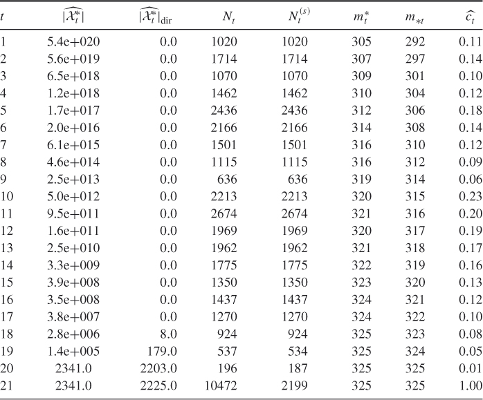
clauses. The exact count is ![]() . A typical dynamics of a run of the adaptive splitting Algorithm 4.2 with
. A typical dynamics of a run of the adaptive splitting Algorithm 4.2 with ![]() ,
, ![]() , and
, and ![]() (single burn-in) is given in Table 4.1.
(single burn-in) is given in Table 4.1.
Table 4.1 Dynamics of Algorithm 4.2 for 3-SAT ![]() model
model

We ran the algorithm 10 times with ![]() ,
, ![]() , and
, and ![]() . The average performance was
. The average performance was
![]()
The direct estimator ![]() gave always the exact result
gave always the exact result ![]() .
.
4.9.1.3 Second Model:  -SAT with Instance Matrix
Our next model is a ![]() -SAT with an instance matrix
-SAT with an instance matrix ![]() taken from www.satlib.org. The exact value is
taken from www.satlib.org. The exact value is ![]() . Table 4.2 presents the dynamics of the adaptive Algorithm 4.2 for this problem.
. Table 4.2 presents the dynamics of the adaptive Algorithm 4.2 for this problem.
Table 4.2 Dynamics of Algorithm 4.2 for the ![]() -SAT with matrix
-SAT with matrix ![]()
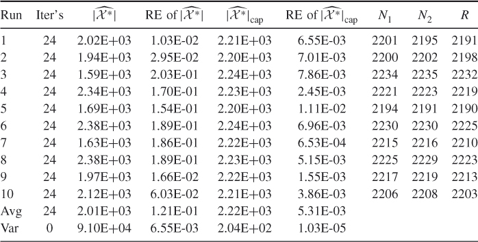
We ran the splitting algorithm 10 times, using sample size ![]() and parameters
and parameters ![]() and
and ![]() for all iterations. We obtained
for all iterations. We obtained
![]()
We also implemented the direct Algorithm 4.5 after the last iteration of the adaptive splitting using ![]() . We obtained
. We obtained
![]()
Table 4.3 presents a comparison of the performances of the adaptive splitting estimator ![]() and its counterpart, the CAP-RECAP estimator, denoted by
and its counterpart, the CAP-RECAP estimator, denoted by ![]() obtained from the capture-recapture Algorithm 4.6. The comparison was done for the same random 3-SAT model with the instance matrix
obtained from the capture-recapture Algorithm 4.6. The comparison was done for the same random 3-SAT model with the instance matrix ![]() . We set
. We set ![]() ,
, ![]() , and
, and ![]() .
.
Table 4.3 Comparison of the Performance of the Adaptive Estimator ![]() and Its CAP-RECAP counterpart
and Its CAP-RECAP counterpart ![]() for the 3-SAT
for the 3-SAT ![]() model
model
Note that the sample ![]() was obtained as soon as soon as Algorithm 4.6 reaches the final level
was obtained as soon as soon as Algorithm 4.6 reaches the final level ![]() , and
, and ![]() was obtained while running it for one more iteration at the same level
was obtained while running it for one more iteration at the same level ![]() . The actual sample sizes
. The actual sample sizes ![]() and
and ![]() were chosen according to the following rule: sample until Algorithm 4.6 screens out 50% of the samples and then stop. It follows from Table 4.3 that for model
were chosen according to the following rule: sample until Algorithm 4.6 screens out 50% of the samples and then stop. It follows from Table 4.3 that for model ![]() this corresponds to
this corresponds to ![]() . It also follows that the relative error of
. It also follows that the relative error of ![]() is about 100 times smaller as compared to
is about 100 times smaller as compared to ![]() .
.
4.9.1.4 Random Graphs with Prescribed Degrees
Random graphs with given vertex degrees is a model for real-world complex networks, including the World Wide Web, social networks, and biological networks. The problem is to find a graph ![]() with
with ![]() vertices, given the degree sequence
vertices, given the degree sequence ![]() with some nonnegative integers. Following [9], a finite sequence
with some nonnegative integers. Following [9], a finite sequence ![]() of non-negative integers is called graphical if there is a labeled simple graph with vertex set
of non-negative integers is called graphical if there is a labeled simple graph with vertex set ![]() in which vertex
in which vertex ![]() has degree
has degree ![]() . Such a graph is called a realization of the degree sequence
. Such a graph is called a realization of the degree sequence ![]() . We are interested in the total number of such realizations for a given degree sequence, hence
. We are interested in the total number of such realizations for a given degree sequence, hence ![]() denotes the set of all graphs
denotes the set of all graphs ![]() with the degree sequence
with the degree sequence ![]() .
.
In order to perform this estimation, we transform the problem into a counting problem by considering the complete graph ![]() of
of ![]() vertices, in which each vertex is connected with all other vertices. Thus, the total number of edges in
vertices, in which each vertex is connected with all other vertices. Thus, the total number of edges in ![]() is
is ![]() , labeled
, labeled ![]() . The random graph problem with prescribed degrees is translated to the problem of choosing those edges of
. The random graph problem with prescribed degrees is translated to the problem of choosing those edges of ![]() such that the resulting graph
such that the resulting graph ![]() matches the given sequence
matches the given sequence ![]() . We set
. We set ![]() when
when ![]() is chosen, and
is chosen, and ![]() , otherwise,
, otherwise, ![]() . So that such an assignment
. So that such an assignment ![]() matches the given degree sequence
matches the given degree sequence ![]() , it holds necessarily that
, it holds necessarily that ![]() , since this is the total number of edges. In other words, the configuration space is
, since this is the total number of edges. In other words, the configuration space is
Let ![]() be the incidence matrix of
be the incidence matrix of ![]() with entries
with entries
It is easy to see that whenever a configuration ![]() satisfies
satisfies ![]() , the associated graph has degree sequence
, the associated graph has degree sequence ![]() . We conclude that the set
. We conclude that the set ![]() is represented by
is represented by
![]()
We first present a small example as illustration. Let ![]() with
with ![]() , and
, and ![]() . After ordering the edges of
. After ordering the edges of ![]() lexicographically, the corresponding incidence matrix is given as
lexicographically, the corresponding incidence matrix is given as
It can be seen that ![]() and
and ![]()
![]() present two solutions of this example.
present two solutions of this example.
For the random graph problem we define the performance function ![]() by
by

where ![]() is the degree of vertex
is the degree of vertex ![]() under the configuration
under the configuration ![]() . Each configuration that satisfies the degree sequence will have a performance function equal to
. Each configuration that satisfies the degree sequence will have a performance function equal to ![]() .
.
The implementation of the Gibbs sampler for this problem is slightly different than for the ![]() -SAT one, in as much as we keep the number of edges in each realization fixed to
-SAT one, in as much as we keep the number of edges in each realization fixed to ![]() . The algorithm below takes care of this requirement and generates a random
. The algorithm below takes care of this requirement and generates a random ![]() .
.
- Input: The prescribed degrees sequence
 .
. - Output: A random
 .
.
The adaptive thresholds in the splitting algorithm are negative, increasing to 0:
![]()
The resulting Gibbs sampler (in Step 3 of the splitting algorithm starting with a configuration ![]() for which
for which ![]() ) can be written as follows.
) can be written as follows.
- Input: A configuration
 with
with  .
. - Output: A uniformly chosen random neighbor with the same property.
For each edge ![]() , while keeping all other edges fixed, do:
, while keeping all other edges fixed, do:
We will apply the splitting algorithm to two problems taken from [9].
4.9.1.5 A Small Problem
For this small problem we have the degree sequence
![]()
The solution can be obtained analytically and is already given in [9], from which we quote:
To count the number of labeled graphs with this degree sequence, note that there are ![]() such graphs with vertex 1 not joined to vertex 2 by an edge (these graphs look like two separate stars), and there are
such graphs with vertex 1 not joined to vertex 2 by an edge (these graphs look like two separate stars), and there are ![]() such graphs with an edge between vertices 1 and 2 (these look like two joined stars with an isolated edge left over). Thus, the total number of realizations of d is
such graphs with an edge between vertices 1 and 2 (these look like two joined stars with an isolated edge left over). Thus, the total number of realizations of d is ![]() .
.
As we will see, the adaptive splitting Algorithm 4.2 easily handles the problem. First we present a typical dynamics (Table 4.4).
Table 4.4 Typical Dynamics of the Splitting Algorithm 4.2 for a small problem using ![]() and
and ![]()
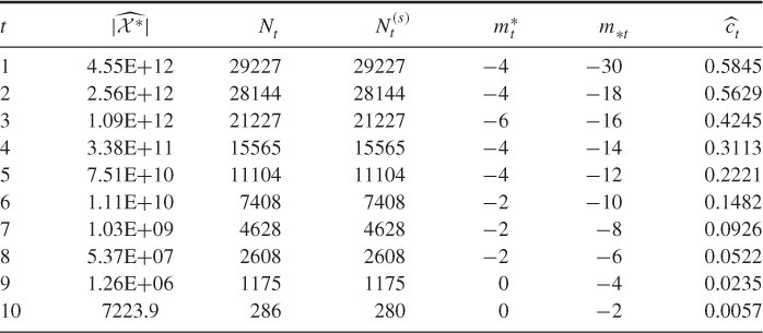
We ran the algorithm 10 times, independently, using sample size ![]() and rarity parameter
and rarity parameter ![]() . The average performance was
. The average performance was
![]()
4.9.1.6 A Large Problem
A much harder instance (see [9]) is defined by
![]()
In [9] the number of such graphs is estimated to be about ![]() . The average performance with the adaptive splitting Algorithm 4.2, based on 10 experiments, using sample size
. The average performance with the adaptive splitting Algorithm 4.2, based on 10 experiments, using sample size ![]() and rarity parameter
and rarity parameter ![]() , was
, was
![]()
4.9.1.7 Binary Contingency Tables
Given are two vectors of positive integers ![]() and
and ![]() such that
such that ![]() for all
for all ![]() ,
, ![]() for all
for all ![]() , and
, and ![]() . A binary contingency table with row sums
. A binary contingency table with row sums ![]() and column sums
and column sums ![]() is a
is a ![]() matrix
matrix ![]() of zero-one entries
of zero-one entries ![]() satisfying
satisfying ![]() for every row
for every row ![]() and
and ![]() for every column
for every column ![]() . The problem is to count all contingency tables.
. The problem is to count all contingency tables.
The extension of the proposed Gibbs sampler for counting the contingency tables follows immediately. We define the configuration space ![]() as the space where all column or row sums are satisfied:
as the space where all column or row sums are satisfied:
Clearly, sampling uniformly on ![]() is straightforward. The sample function
is straightforward. The sample function ![]() is defined by
is defined by
that is, the difference of the row sums ![]() with the target
with the target ![]() if the column sums are right, and vice versa.
if the column sums are right, and vice versa.
The Gibbs sampler is similar to random graphs with prescribed degrees.
- Input: A matrix realization
 with performance value
  .
. - Output: A uniformly chosen random neighbor with the same property.
For each column ![]() and for each 1-entry in this column (
and for each 1-entry in this column (![]() ) do:
) do:
In this way we keep the column sums correct. Similarly, when we started with a matrix configuration with all row sums correct, we execute these steps for each row and swap 1 and 0 per row.
4.9.1.8 Model 1
The data are ![]() with row and column sums
with row and column sums
![]()
The true count value is known to be ![]() (reported in [28]). Table 4.5 presents a typical dynamics of the adaptive splitting Algorithm 4.2 for Model 1 using
(reported in [28]). Table 4.5 presents a typical dynamics of the adaptive splitting Algorithm 4.2 for Model 1 using ![]() and
and ![]() .
.
Table 4.5 Typical Dynamics of the Splitting Algorithm 4.2 for model 1 using ![]() and
and ![]()

The average performance based on 10 experiments using sample size ![]() and rarity parameter
and rarity parameter ![]() was
was
![]()
4.9.1.9 Model 2
Consider the problem of counting tables with Darwin's finch data as marginal sums given in Chen et al. [28]. The data are ![]() with row and columns sums
with row and columns sums
![]()
The true count value in [28] is ![]() . The average performance based on 10 independent experiments using sample size
. The average performance based on 10 independent experiments using sample size ![]() and rarity parameter
and rarity parameter ![]() was
was
![]()
4.9.1.10 Vertex Coloring
Vertex coloring is a problem of coloring the vertices of a graph ![]() consisting of
consisting of ![]() nodes and
nodes and ![]() edges, such that neighboring vertices have different colors. The set of colors has a size
edges, such that neighboring vertices have different colors. The set of colors has a size ![]() . For more details on vertex coloring see Section A.1.1.
. For more details on vertex coloring see Section A.1.1.
- Input: A graph
 with proper coloring.
 - Output: A uniformly chosen random neighbor with the same property.
For each vertex ![]() do:
do:
We consider here two coloring models: a small one and one of moderate size.
4.9.1.11 First Model:  Vertices,
  Edges,
  Colors
The graph ![]() has the following
has the following ![]() adjacency matrix.
adjacency matrix.
The performance is based on 10 independent experiments using sample size ![]() and rarity parameter
and rarity parameter ![]() , was
, was
![]()
Note that the splitting procedure starts with the set ![]() consisting of all feasible colorings of the graph
consisting of all feasible colorings of the graph ![]() (see Section A.1.1). Thus,
(see Section A.1.1). Thus, ![]() . We obtain, in this case, that the probability equals
. We obtain, in this case, that the probability equals
![]()
Because ![]() is not a rareevent, the crude Monte Carlo method can also be used here. The performance of the CMC estimator based on 10 independent runs with
is not a rareevent, the crude Monte Carlo method can also be used here. The performance of the CMC estimator based on 10 independent runs with ![]() and
and ![]() was
was
![]()
It follows the RE of the CMC is about 3 times larger than its counterpart, the splitting Algorithm 4.2.
4.9.1.12 Second Model:  Vertices,
  Edges,
We next consider a larger and sparser coloring model, one with ![]() vertices,
vertices, ![]() edges, and
edges, and ![]() .
.
For this model, we applied the adaptive splitting Algorithm 4.2 with sample size ![]() , rarity parameter
, rarity parameter ![]() , and burn-in parameter
, and burn-in parameter ![]() . The direct algorithm was implemented immediately after the last iteration of the adaptive splitting, using again
. The direct algorithm was implemented immediately after the last iteration of the adaptive splitting, using again ![]() . Table 4.6 presents the dynamics for a single run of the splitting Algorithm 4.2.
. Table 4.6 presents the dynamics for a single run of the splitting Algorithm 4.2.
Table 4.6 Dynamics of Algorithm 4.2 for 4-Coloring graph with ![]() nodes
nodes
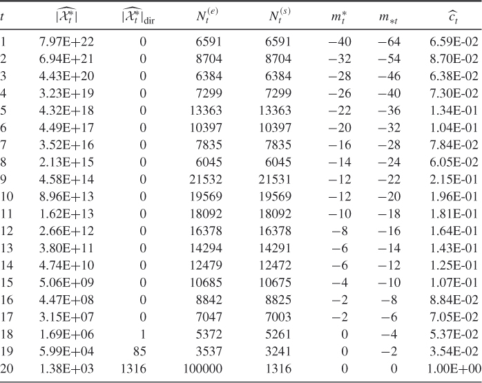
The average performance based on 10 independent experiments was
![]()
The direct splitting algorithm results in ![]() with RE
with RE ![]() .
.
4.9.1.13 Permanent
The permanent of a general ![]() matrix
matrix ![]() is defined as
is defined as
4.27 
where ![]() is the set of all permutations
is the set of all permutations ![]() of
of ![]() .
.
Note that, in contrast to the Hamiltonian cycle problem, the diagonal elements of the matrix ![]() need not to be zeros. The
need not to be zeros. The ![]() permutations with the corresponding product values
permutations with the corresponding product values ![]() are given in Table 4.7. The permanent is
are given in Table 4.7. The permanent is ![]() . The values of the performance function
. The values of the performance function ![]() with all six possible permutation vectors
with all six possible permutation vectors ![]() are given in Table 4.8.
are given in Table 4.8.![]()
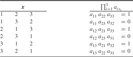
To apply the Gibbs sampler for the permanent problem, we adopt the concept of “neighboring” elements (see, for example, Chapter 10 of Ross [99]) and in particular the concept of 2-opt heuristic [108]. More precisely, given a point (tour) ![]() of length
of length ![]() generated by the pdf
generated by the pdf ![]() , the conditional Gibbs sampling updates the existing tour
, the conditional Gibbs sampling updates the existing tour ![]() to
to ![]() , where
, where ![]() is generated from
is generated from ![]() and where
and where ![]() is the same as
is the same as ![]() with the exception that the points
with the exception that the points ![]() and
and ![]() in
in ![]() are interchanged. We accept the tour
are interchanged. We accept the tour ![]() if
if ![]() , otherwise, we leave the tour
, otherwise, we leave the tour ![]() the same. If
the same. If ![]() is accepted, we update the cost function
is accepted, we update the cost function ![]() (for
(for ![]() ) accordingly. We found empirically that, in order for the tours
) accordingly. We found empirically that, in order for the tours ![]() to be distributed approximately uniformly (at each subspace
to be distributed approximately uniformly (at each subspace ![]() ), we used
), we used ![]() trials.
trials.
The Gibbs sampler may be summarized as follows:
- Input: Given a permutation
 and
and  .
. - Output: A uniformly chosen random neighbor with the same property.
For each ![]() and
and ![]()
![]() do:
do:
We applied the adaptive splitting Algorithm 4.2 to a problem with an instance matrix ![]() matrix. We took a sample size
matrix. We took a sample size ![]() and set the rarity parameter
and set the rarity parameter ![]() and burn-in parameter
and burn-in parameter ![]() . The average performance based on 10 experiments was
. The average performance based on 10 experiments was
![]()
The direct estimator was implemented immediately after the last iteration of the adaptive splitting, using again ![]() . The average performance of the direct algorithm was
. The average performance of the direct algorithm was ![]() with RE
with RE ![]() .
.
4.9.1.14 Hamiltonian Cycles
We solve the Hamiltonian cycles problem by applying the 2-opt heuristic used for the permanent. In counting Hamiltonian cycles we simulated an associated permanent problem by making use of the following observations:
- The set of Hamiltonian cycles of length
 represents a subset of the associated permanent set of trajectories.
 - The latter set is formed from cycles of length
 .
.
It follows that, in order to count the number of Hamiltonian cycles for a given matrix ![]() , one can use the following simple procedure:
, one can use the following simple procedure:
Below we present simulation results for two ![]() models. We choose
models. We choose ![]() ,
, ![]() and
and ![]() . The results are based on the averages of 10 experiments. The adaptive splitting algorithm results in
. The results are based on the averages of 10 experiments. The adaptive splitting algorithm results in
![]()
while the direct algorithm results in
![]()
4.9.1.15 Volume of a Polytope
Here we present numerical results with the splitting Algorithm 4.2, on the volume of a polytope defined as ![]() . We assume in addition that all components
. We assume in addition that all components ![]() . By doing so the polytope
. By doing so the polytope ![]() will be inside the unit
will be inside the unit ![]() -dimensional cube and therefore its volume is very small (rare-event probability) relative to that of the unit cube. In general, however, before implementing the Gibbs sampler, one must find the minimal
-dimensional cube and therefore its volume is very small (rare-event probability) relative to that of the unit cube. In general, however, before implementing the Gibbs sampler, one must find the minimal ![]() -dimensional box, which contains the polytope, that is, for each
-dimensional box, which contains the polytope, that is, for each ![]() , one must find the values
, one must find the values ![]() of the minimal box satisfying
of the minimal box satisfying ![]() . This can be done by solving for each
. This can be done by solving for each ![]() the following two linear programs:
the following two linear programs:
4.29 ![]()
4.30 ![]()
and
4.31 ![]()
4.32 ![]()
We consider two models.
4.9.1.16 First Model
4.33 
Table 4.9 presents the dynamics of a single run of the splitting Algorithm 4.2 with ![]() and
and ![]() . The results are self-explanatory.
. The results are self-explanatory.
Table 4.9 Dynamics of single run of splitting Algorithm 4.2
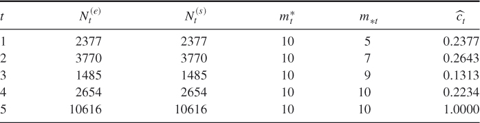
In this model, we also executed the crude Monte Carlo, for which we took a sample ![]() . The results of 10 experiments are
. The results of 10 experiments are
4.9.1.17 Second Model
This problem involves a ![]() matrix, whose main part,
matrix, whose main part, ![]() , comprises the first 60 column vectors of matrix
, comprises the first 60 column vectors of matrix ![]() with 0-1 entries and the rightmost column corresponds to the vector
with 0-1 entries and the rightmost column corresponds to the vector ![]() . Running the splitting Algorithm 4.2 for 10 independent runs, each with
. Running the splitting Algorithm 4.2 for 10 independent runs, each with ![]() and
and ![]() , we obtained average performance
, we obtained average performance
![]()
4.9.2 Combinatorial Optimization
4.9.2.1 Traveling Salesman Problem
We now present some numerical results obtained with splitting Algorithm 4.2 while using the 2-opt heuristics. The models are taken from http://www.iwr.uni-heidelberg.de/groups/comopt/software/TSPLIB95/atsp.
All our results are based on 10 independent runs with the random Gibbs sampler. Below, we consider the ftv33 model with ![]() nodes and the best-known solution, equal to 1286. We used in our simulation studies
nodes and the best-known solution, equal to 1286. We used in our simulation studies ![]() and
and ![]() . We found that the accuracy with
. We found that the accuracy with ![]() is higher than for
is higher than for ![]() , but the CPU time in the latter increased by about 20%. We also found that the accuracy of the splitting Algorithm 4.2 is quite sensitive to
, but the CPU time in the latter increased by about 20%. We also found that the accuracy of the splitting Algorithm 4.2 is quite sensitive to ![]() ,
, ![]() , and
, and ![]() . Below are some results:
. Below are some results:
 ,
,  , and
, and  . The results are

The CPU was 25 sec for a run.
 ,
,  , and
, and  . In this case, the 2-opt heuristic results in the best-known solution is
  in all 10 runs.
 ,
,  , and
, and  . The results are

 ,
,  , and
, and  . The results are

 ,
,  , and
, and  . The results are
 (This is the worst case, with relative error about 7%.)
4.9.2.2 Knapsack Problem
Consider the Sento1.dat knapsack problem given in http://people.brunel.ac.uk/mastjjb/jeb/orlib/files/mknap2.txt. The problem has 30 constraints and 60 variables. We ran the splitting Algorithm 4.4 for 10 independent runs with ![]() ,
, ![]() ,
, ![]() , and we found that it discovers the best-known solution. We also ran it for various integer problems and always found that the results coincided with the best-known solution.
, and we found that it discovers the best-known solution. We also ran it for various integer problems and always found that the results coincided with the best-known solution.
4.9.3 Reliability Models
To estimate the system unreliability parameter ![]() , we use in all our numerical experiments the exponential pdf
, we use in all our numerical experiments the exponential pdf ![]() with the rates
with the rates ![]() , where
, where ![]() is the underlying Bernoulli vector.
is the underlying Bernoulli vector.
Our numerical results are given for a dodecahedron graph in Figure 4.11 and a lattice graph. Note that an ![]() graph has
graph has ![]() rows containing
rows containing ![]() nodes each, arranged in a rectangular lattice. Each node is connected to its neighbors on the left, right, above, and below, where they exist. As an illustration, a
nodes each, arranged in a rectangular lattice. Each node is connected to its neighbors on the left, right, above, and below, where they exist. As an illustration, a ![]() lattice graph is presented in Figure 4.12. In all our numerical experiments, we take the terminals to be the upper-left and the lower-right nodes of the corresponding lattice graph.
lattice graph is presented in Figure 4.12. In all our numerical experiments, we take the terminals to be the upper-left and the lower-right nodes of the corresponding lattice graph.
Figure 4.11 The dodecahedron graph.

Figure 4.12 A ![]() lattice graph, with 40 nodes and 67 edges.
lattice graph, with 40 nodes and 67 edges.
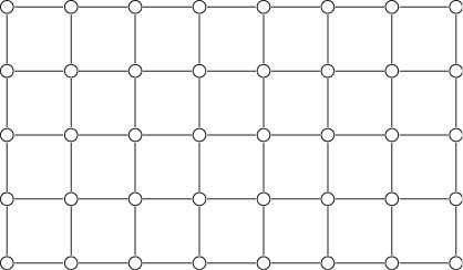
To estimate the unreliability parameter ![]() we run both models for 10 independent scenarios.
we run both models for 10 independent scenarios.
4.9.3.1 Dodecahedron Graph with Terminal Nodes 
We considered the following two cases:
![]()
The average CPU time was ![]() seconds and the relative error was
seconds and the relative error was ![]() .
.
![]()
The average CPU time was ![]() seconds and the relative error was about
seconds and the relative error was about ![]() .
.
4.9.3.2 Lattice  Graph with
We considered the following two cases:
![]()
The average CPU time was ![]() seconds and the relative error was
seconds and the relative error was ![]() .
.
![]()
The average CPU time was ![]() seconds and the relative error was
seconds and the relative error was ![]() .
.
4.10 Appendix: Gibbs Sampler
In this appendix, we show how to sample from a given joint pdf ![]() using the Gibbs sampler, where instead of proceeding with
using the Gibbs sampler, where instead of proceeding with ![]() directly, which might be very difficult, one samples from one-dimensional conditional pdfs
directly, which might be very difficult, one samples from one-dimensional conditional pdfs ![]() , which is typically much simpler.
, which is typically much simpler.
Two basic versions of the Gibbs sampler [108] are available: systematic and random. In the former, the components of the vector ![]() are updated in a fixed, say increasing, order, while in the latter they are chosen randomly according to a discrete uniform
are updated in a fixed, say increasing, order, while in the latter they are chosen randomly according to a discrete uniform ![]() -point pdf. Below we present the systematic version, where for a given vector
-point pdf. Below we present the systematic version, where for a given vector ![]() , one generates a new vector
, one generates a new vector ![]() with the same distribution
with the same distribution ![]() as follows:
as follows:
Iterating with Algorithm 4.15, the Gibbs sampler generates (subject to some mild conditions, see [108]), a sample distributed ![]() .
.
We denote for convenience each conditional pdf ![]() by
by ![]() , where
, where ![]() denotes conditioning on all random variables except the
denotes conditioning on all random variables except the ![]() -th component.
-th component.
We next present a random Gibbs sampler taken from (Ross, 2006) for estimating each ![]() according to (4.11), that is,
according to (4.11), that is,
For many rare-event and counting problems, generation from the conditional pdf ![]() can be achieved directly, that is, skipping Step 5. This should obviously speed things up.
can be achieved directly, that is, skipping Step 5. This should obviously speed things up.