
Appendix A
Additional Topics
A.1 Combinatorial Problems
Combinatorics is a branch of mathematics concerning the study of finite or countable discrete structures and, in particular, how the discrete structures can be combined or arranged. Aspects of combinatorics include counting the structures of a given kind and size, deciding when certain criteria can be met, and combinatorial optimization.
Combinatorial problems arise in many areas of pure mathematics, notably in algebra, probability theory, topology, and geometry, and combinatorics also has many applications in optimization, computer science, ergodic theory, and statistical physics. In the later twentieth century, however, powerful and general theoretical methods were developed, making combinatorics into an independent branch of mathematics in its own right. Combinatorics is used frequently in computer science to obtain formulas and estimates in the analysis of algorithms.
An important part of the study is to analyze the complexity of the proposed algorithms. In combinatorics, we are interested in particular arrangements or combinations of the objects. For instance, neighboring countries are colored differently when drawn on a map. We might be interested in the minimal number of colors needed or in how many different ways we can color the map when given a number of colors to use.
Knuth [68], page 1 distinguishes five issues of concern in combinatorics:
In this book we focus on issues (i), (iii), and (v). Issue (i) is also called the decision problem; issue (iii) is also known as the counting problem. In particular, we consider combinatorial problems that can be modeled by an optimization program and, in fact, most often by an integer linear program. For that purpose, we denote by ![]() the set of feasible solutions of the problem, and we assume that it is a subset of an
the set of feasible solutions of the problem, and we assume that it is a subset of an ![]() -dimensional integer vector space and that is given by the following linear integer constraints (cf. (1.1)):
-dimensional integer vector space and that is given by the following linear integer constraints (cf. (1.1)):

where,
- Decision making: is
 nonempty?
 - Counting: calculate
 .
. - Optimization: solve
 for a given objective or performance function
  .
.
In this book, we describe in detail various problems, algorithms, and mathematical aspects that are related to the issues (i)–(iii) and associated with the problem (A.1). The following two sections deal with a sample of well-known counting and optimization problems, respectively.
A.1.1 Counting
In this section, we present details of the satisfiability problem, independent set problem, vertex coloring problem, Hamiltonian cycle problem, the knapsack problem, and the permanent problem.
A.1.1.1 Satisfiability Problem
The most common satisfiability problem (SAT) comprises the following two components:
- A set of
 boolean variables
  , representing statements that can either be TRUE (
 ) or FALSE (
 ). The negation (the logical NOT) of a variable
  is denoted by
  . A variable or its negation is called a literal.
 - A set of
 distinct clauses
  of the form
 , where the
  's are the literals of the
  variables, and the
  denotes the logical OR operator.
The binary vector ![]() is called a truth assignment, or simply an assignment. Thus,
is called a truth assignment, or simply an assignment. Thus, ![]() assigns truth to
assigns truth to ![]() and
and ![]() assigns truth to
assigns truth to ![]() , for each
, for each ![]() . The simplest SAT problem can now be formulated as follows: find a truth assignment
. The simplest SAT problem can now be formulated as follows: find a truth assignment ![]() such that all clauses are true.
such that all clauses are true.
Denoting the logical AND operator by ![]() , we can represent the above SAT problem via a single formula as
, we can represent the above SAT problem via a single formula as
where ![]() is the number of literals in clause
is the number of literals in clause ![]() and
and ![]() are the literals of the
are the literals of the ![]() variables in clause
variables in clause ![]() . The SAT formula is then said to be in conjunctive normal form (CNF). When all clauses have exactly the same number
. The SAT formula is then said to be in conjunctive normal form (CNF). When all clauses have exactly the same number ![]() of literals per clause, we say that we deal with the
of literals per clause, we say that we deal with the ![]() -SAT problem.
-SAT problem.
The problem of deciding whether there exists a valid assignment, and, indeed, providing such a vector is called the SAT-assignment problem and is ![]() -complete [92]. We are concerned with the harder problem to count all valid assignments, which is
-complete [92]. We are concerned with the harder problem to count all valid assignments, which is ![]() -complete.
-complete.
SAT problems can be converted into the framework of a solution set given by linear constraints. Define the ![]() matrix
matrix ![]() with entries
with entries ![]() by
by
Furthermore, let ![]() be the
be the ![]() -vector with entries
-vector with entries ![]() . Then it is easy to see that, for any configuration
. Then it is easy to see that, for any configuration ![]() ,
,
![]()
Thus, the SAT problem presents a particular case of the integer linear program with constraints given in (A.1).
A.1.1.2 Independent Sets
Consider a graph ![]() with
with ![]() nodes and
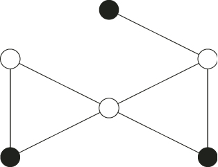
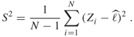
nodes and ![]() edges. Our goal is to count the number of independent node sets of this graph. A node set is called independent if no two nodes are connected by an edge, that is, no two nodes are adjacent; see Figure A.1 for an illustration of this concept.
edges. Our goal is to count the number of independent node sets of this graph. A node set is called independent if no two nodes are connected by an edge, that is, no two nodes are adjacent; see Figure A.1 for an illustration of this concept.
Figure A.1 The black nodes form an independent set inasmuch as they are not adjacent to each other.
The independent set problem can be converted into the family of integer programming problems (A.1) by considering the transpose of the incidence matrix ![]() . The nodes are labeled
. The nodes are labeled ![]() ; the edges are labeled
; the edges are labeled ![]() . Then
. Then ![]() is a
is a ![]() matrices of zeros and ones with
matrices of zeros and ones with ![]() iff the edge
iff the edge ![]() and node
and node ![]() are incident. The decision vector
are incident. The decision vector ![]() denotes which nodes belong to the independent set. Finally, let
denotes which nodes belong to the independent set. Finally, let ![]() be the
be the ![]() -column vector with entries
-column vector with entries ![]() for all
for all ![]() . Then it is easy to see that for any configuration
. Then it is easy to see that for any configuration ![]()
![]()
Having formulated the problem set ![]() as the feasible set of an integer linear program with bounded variables, we can apply the procedure mentioned in Section 4.1 for constructing a sequence of decreasing sets (4.1) in order to start the splitting method.
as the feasible set of an integer linear program with bounded variables, we can apply the procedure mentioned in Section 4.1 for constructing a sequence of decreasing sets (4.1) in order to start the splitting method.
An alternative construction of the sequence of decreasing sets (4.1) is the following. Let ![]() be the set of the first
be the set of the first ![]() edges and define the associated subgraph
edges and define the associated subgraph ![]() ,
, ![]() . Note that
. Note that ![]() , and that
, and that ![]() is obtained from
is obtained from ![]() by adding the edge
by adding the edge ![]() , which is not in
, which is not in ![]() . Define
. Define ![]() to be the set of the independent sets of
to be the set of the independent sets of ![]() , then clearly
, then clearly ![]() . Here
. Here ![]() , because
, because ![]() has no edges and thus every subset of
has no edges and thus every subset of ![]() is an independent set, including the empty set.
is an independent set, including the empty set.
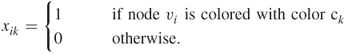
A.1.1.3 Vertex Coloring
Given a graph ![]() with
with ![]() nodes
nodes ![]() , and
, and ![]() edges
edges ![]() , color the nodes of
, color the nodes of ![]() with at most a
with at most a ![]() colors given from a set of colors
colors given from a set of colors ![]() , such that for each edge
, such that for each edge ![]() , nodes
, nodes ![]() and
and ![]() have different colors. We shall show how to cast the node coloring problem into the framework (A.1). Define the decision variables
have different colors. We shall show how to cast the node coloring problem into the framework (A.1). Define the decision variables ![]() for
for ![]() and
and ![]() by
by
Then, ![]() iff
iff
An alternative to (A.2) framework can be obtained by arguing as follows. Define decision variables ![]() for
for ![]() by
by
![]()
Then, ![]() iff
iff
A.3 ![]()
The procedure for node coloring via the randomized algorithm is the same as for the independent sets problem. Again, let ![]() be the set of the first
be the set of the first ![]() edges and let
edges and let ![]() be the associated subgraph,
be the associated subgraph, ![]() . Note that
. Note that ![]() , and that
, and that ![]() is obtained from
is obtained from ![]() by adding the edge
by adding the edge ![]() . Define
. Define ![]() to be the set of the node colorings of
to be the set of the node colorings of ![]() , then clearly
, then clearly ![]() . Here
. Here ![]() , because
, because ![]() has no edges and thus we can color any node with any color.
has no edges and thus we can color any node with any color.
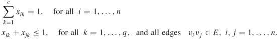
A.1.1.4 Hamiltonian Cycles
Given a graph ![]() with
with ![]() nodes and
nodes and ![]() edges, find all Hamiltonian cycles. Figure A.2 presents a graph with eight nodes and several Hamiltonian cycles, one of which is marked in bold lines.
edges, find all Hamiltonian cycles. Figure A.2 presents a graph with eight nodes and several Hamiltonian cycles, one of which is marked in bold lines.
Figure A.2 A Hamiltonian graph. The bold edges form a Hamiltonian cycle.
A.1.1.5 Permanent
Let ![]() be a
be a ![]() matrix consisting of zeros and ones only. The permanent of
matrix consisting of zeros and ones only. The permanent of ![]() is defined by
is defined by
A.4 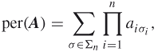
where ![]() is the set of all permutations
is the set of all permutations ![]() of
of ![]() .
.
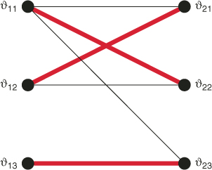
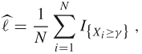
It is well known that the permanent of ![]() equals the number of perfect matchings in a balanced bipartite graph
equals the number of perfect matchings in a balanced bipartite graph ![]() with matrix
with matrix ![]() as its biadjacency matrix [90]: two disjoint sets of nodes
as its biadjacency matrix [90]: two disjoint sets of nodes ![]() and
and ![]() , where
, where ![]() iff
iff ![]() . Recall that a matching is a collection of edges
. Recall that a matching is a collection of edges ![]() such that each node occurs at most once in
such that each node occurs at most once in ![]() . A perfect matching is a matching of size
. A perfect matching is a matching of size ![]() .
.
To cast the bipartite perfect matching problem in an integer linear program, we define the decision variables ![]() by
by
Let ![]() be the set of all perfect matchings of the bipartite graph associated with the given binary matrix
be the set of all perfect matchings of the bipartite graph associated with the given binary matrix ![]() . Then
. Then ![]() iff
iff
A.5 
As an example, let ![]() be the
be the ![]() matrix
matrix
A.6 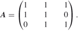
The corresponding bipartite graph is given in Figure A.3. The graph has three perfect matchings, one of which is displayed in the figure.
Figure A.3 A bipartite graph. The bold edges form a perfect matching.
A.1.1.6 Knapsack Problem
Given items of sizes ![]() and a positive integer
and a positive integer ![]() , find the numbers of vectors
, find the numbers of vectors ![]() , such that
, such that
The integer ![]() represents the size of the knapsack, and
represents the size of the knapsack, and ![]() indicates whether or not item
indicates whether or not item ![]() is placed in it. Let
is placed in it. Let ![]() denote the set of all feasible solutions, that is, all different combinations of items that can be placed in the knapsack without exceeding its capacity. The goal is to determine
denote the set of all feasible solutions, that is, all different combinations of items that can be placed in the knapsack without exceeding its capacity. The goal is to determine ![]() .
.
A.1.2 Combinatorial Optimization
In this section, we present details of the max-cut problem, the traveling salesman problem, Internet security problem, set covering/partitioning/packing problem, knapsack problems, the maximum satisfiability problem, the weighted matching problem, and graph coloring problems.
A.1.2.1 Max-Cut Problem
The maximal-cut (max-cut) problem in a graph can be formulated as follows. Given a graph ![]() with a set of nodes
with a set of nodes ![]() , a set of edges
, a set of edges ![]() between the nodes, and a weight function on the edges,
between the nodes, and a weight function on the edges, ![]() . The problem is to partition the nodes into two subsets
. The problem is to partition the nodes into two subsets ![]() and
and ![]() such that the sum of the weights
such that the sum of the weights ![]() of the edges going from one subset to the other is maximized:
of the edges going from one subset to the other is maximized:
A cut can be conveniently represented via its corresponding cut vector ![]() , where
, where ![]() if node
if node ![]() belongs to same partition as
belongs to same partition as ![]() , and
, and ![]() else. For each cut vector
else. For each cut vector ![]() , let
, let ![]() be the partition of
be the partition of ![]() induced by
induced by ![]() , such that
, such that ![]() contains the set of nodes
contains the set of nodes ![]() . Unless stated otherwise, we let
. Unless stated otherwise, we let ![]() (thus,
(thus, ![]() ).
).
Let ![]() be the set of all cut vectors
be the set of all cut vectors ![]() and let
and let ![]() be the corresponding cost of the cut. Then,
be the corresponding cost of the cut. Then,
A.7 
When we do not specify, we assume that the graph is undirected. However, when we deal with a directed graph, the cost of a cut ![]() includes both the cost of the edges from
includes both the cost of the edges from ![]() to
to ![]() and from
and from ![]() to
to ![]() . In this case, the cost corresponding to a cut vector
. In this case, the cost corresponding to a cut vector ![]() is, therefore,
is, therefore,
A.8 
A.1.2.2 Traveling Salesman Problem
The traveling salesman problem (TSP) can be formulated as follows. Consider a weighted graph ![]() with
with ![]() nodes, labeled
nodes, labeled ![]() . The nodes represent cities, and the edges represent the roads between the cities. Each edge from
. The nodes represent cities, and the edges represent the roads between the cities. Each edge from ![]() to
to ![]() has weight or cost
has weight or cost ![]() , representing the length of the road. The problem is to find the shortest tour that visits all the cities exactly once and such that the starting city is also the terminating one.
, representing the length of the road. The problem is to find the shortest tour that visits all the cities exactly once and such that the starting city is also the terminating one.
Let ![]() be the set of all possible tours and let
be the set of all possible tours and let ![]() be the total length of tour
be the total length of tour ![]() . We can represent each tour via a permutation
. We can represent each tour via a permutation ![]() with
with ![]() . Mathematically, the TSP reads as
. Mathematically, the TSP reads as
A.9 
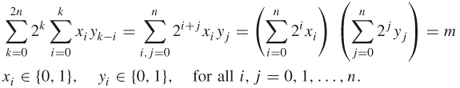
A.1.2.3 RSA or Internet Security Problem
The RSA, also called the Internet security problem, reads as follows: find two primes, provided we are given a large integer ![]() known to be a product of these primes. Clearly, we can write the given number
known to be a product of these primes. Clearly, we can write the given number ![]() in the binary system with
in the binary system with ![]() -bit integers as
-bit integers as
![]()
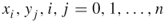
Mathematically, the problem reads as follows: find binary ![]() such that
such that
Remarks:
- The problem (A.10) can be formulated for any basis, say for a decimal rather than a binary one.
- To have a unique solution, we can impose in addition the constraint
 .
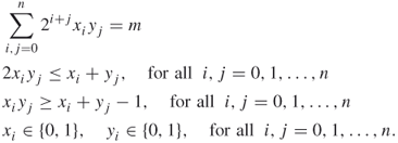
. - The RSA problem can also be formulated as:
Find binary
 such that
A.11
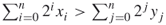
Let ![]() . In this case, the primes are
. In this case, the primes are ![]() and
and ![]() . We can write them as
. We can write them as
![]()
and
![]()
respectively. In this case ![]() and the program (A.10) reduces to:
and the program (A.10) reduces to:
Find binary ![]() such that
such that
A.12 
The program should deliver the unique solution
![]()
Note that we should consider ![]() and
and ![]() as the same solution as the previous one.
as the same solution as the previous one.![]()
A.1.2.4 Set Covering, Set Packing, and Set Partitioning
Consider a finite set ![]() and let
and let ![]() ,
, ![]() be a collection of subsets of the set
be a collection of subsets of the set ![]() where
where ![]() . A subset
. A subset ![]() is called a cover of
is called a cover of ![]() if
if ![]() , and is called a packing of
, and is called a packing of ![]() if
if ![]() for all
for all ![]() and
and ![]() . If
. If ![]() is both a cover and packing, it is called a partitioning.
is both a cover and packing, it is called a partitioning.
Suppose ![]() is the cost associated with
is the cost associated with ![]() . Then the set covering problem is to find a minimum cost cover. If
. Then the set covering problem is to find a minimum cost cover. If ![]() is the value or weight of
is the value or weight of ![]() , then the set packing problem is to find a maximum weight or value packing. Similarly, the set partitioning problem is to find a partitioning with minimum cost. These problems can be formulated as zero-one linear integer programs as shown below. For all
, then the set packing problem is to find a maximum weight or value packing. Similarly, the set partitioning problem is to find a partitioning with minimum cost. These problems can be formulated as zero-one linear integer programs as shown below. For all ![]() and
and ![]() , let
, let
and
Then, the set covering, set packing, and set partitioning formulations are given by

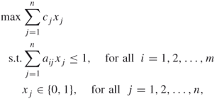
and

respectively.
A.1.2.5 Maximum Satisfiability Problem
The satisfiability problem has been introduced in Section A.1.1. When there is no feasible solution, one might be interested in finding an assignment of truth values to the variables that satisfies the maximum number of clauses, called the MAX-SAT problem.
If one associates a weight ![]() to each clause
to each clause ![]() , one obtains the weighted MAX-SAT problem, denoted by MAX W-SAT. The assignment of truth values to the
, one obtains the weighted MAX-SAT problem, denoted by MAX W-SAT. The assignment of truth values to the ![]() variables that maximizes the sum of the weights of the satisfied clauses is determined. Of course, MAX-SAT is contained in MAX W-SAT (all weights are equal to one). When all clauses have exactly the same number
variables that maximizes the sum of the weights of the satisfied clauses is determined. Of course, MAX-SAT is contained in MAX W-SAT (all weights are equal to one). When all clauses have exactly the same number ![]() of literals per clause, we say that we deal with the MAX-
of literals per clause, we say that we deal with the MAX-![]() -SAT problem, or MAX W-
-SAT problem, or MAX W-![]() -SAT in the weighted case.
-SAT in the weighted case.
The MAX W-SAT problem has a natural integer linear programming formulation (ILP). Recall the boolean decision variables ![]() , meaning TRUE (
, meaning TRUE (![]() ) and FALSE (
) and FALSE (![]() ). Let the boolean variable
). Let the boolean variable ![]() if clause
if clause ![]() is satisfied,
is satisfied, ![]() otherwise. The integer linear program is
otherwise. The integer linear program is

where ![]() and
and ![]() denote the set of indices of variables that appear un-negated and negated in clause
denote the set of indices of variables that appear un-negated and negated in clause ![]() , respectively.
, respectively.
Because the sum of the ![]() is maximized and because each
is maximized and because each ![]() appears as the right-hand side of one constraint only,
appears as the right-hand side of one constraint only, ![]() will be equal to one if and only if clause
will be equal to one if and only if clause ![]() is satisfied.
is satisfied.
A.1.2.6 Weighted Matching
Let ![]() be a graph with
be a graph with ![]() nodes (
nodes (![]() even), and let
even), and let ![]() be a weight function on the edges, then the (general weighted) matching problem is formulated as
be a weight function on the edges, then the (general weighted) matching problem is formulated as
A.13 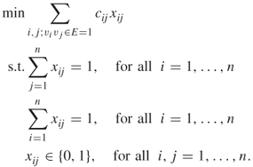
A.1.2.7 Knapsack Problems
All knapsack problems consider a set of items with associated profit ![]() and weight
and weight ![]() . A subset of the items is to be chosen such that the weight sum does not exceed the capacity
. A subset of the items is to be chosen such that the weight sum does not exceed the capacity ![]() of the knapsack, and such that the largest possible profit sum is obtained. We will assume that all coefficients
of the knapsack, and such that the largest possible profit sum is obtained. We will assume that all coefficients ![]() ,
, ![]() ,
, ![]() are positive integers, although weaker assumptions may sometimes be handled in the individual problems.
are positive integers, although weaker assumptions may sometimes be handled in the individual problems.
The 0-1 knapsack problem is the problem of choosing some of the ![]() items such that the corresponding profit sum is maximized without the weight sum exceeding the capacity
items such that the corresponding profit sum is maximized without the weight sum exceeding the capacity ![]() . Thus, it may be formulated as the following maximization problem:
. Thus, it may be formulated as the following maximization problem:
A.14 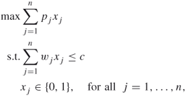
where ![]() is a binary variable having value
is a binary variable having value ![]() if item
if item ![]() should be included in the knapsack, and
should be included in the knapsack, and ![]() otherwise. If we have a bounded amount
otherwise. If we have a bounded amount ![]() of each item type
of each item type ![]() , then the bounded knapsack problem appears:
, then the bounded knapsack problem appears:
A.15 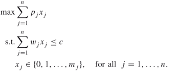
Here ![]() gives the amount of each item type that should be included in the knapsack in order to obtain the largest objective value. The unbounded knapsack problem is a special case of the bounded knapsack problem, since an unlimited amount of each item type is available:
gives the amount of each item type that should be included in the knapsack in order to obtain the largest objective value. The unbounded knapsack problem is a special case of the bounded knapsack problem, since an unlimited amount of each item type is available:
A.16 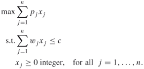
Actually, any variable ![]() of an unbounded knapsack problem will be bounded by the capacity
of an unbounded knapsack problem will be bounded by the capacity ![]() , as the weight of each item is at least one. But, generally, there is no benefit by transforming an unbounded knapsack problem into its bounded version.
, as the weight of each item is at least one. But, generally, there is no benefit by transforming an unbounded knapsack problem into its bounded version.
The most general form of a knapsack problem is the multiconstrained knapsack problem, which is basically a general integer programming problem, where all coefficients ![]() ,
, ![]() , and
, and ![]() are non-negative integers. Thus, it may be formulated as
are non-negative integers. Thus, it may be formulated as
A.17 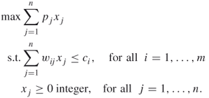
The quadratic knapsack problem presented is an example of a knapsack problem with a quadratic objective function. It may be stated as
A.18 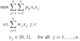
Here, ![]() is the profit obtained if both items
is the profit obtained if both items ![]() and
and ![]() are chosen, while
are chosen, while ![]() is the weight of item
is the weight of item ![]() . The quadratic knapsack problem is a knapsack counterpart to the quadratic assignment problem, and theproblem has several applications in telecommunication and hydrological studies.
. The quadratic knapsack problem is a knapsack counterpart to the quadratic assignment problem, and theproblem has several applications in telecommunication and hydrological studies.
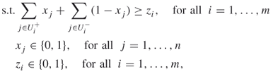
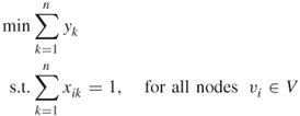
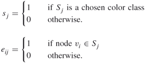
A.1.2.8 Graph Coloring
Similar to many combinatorial optimization problems, the graph coloring problem has several mathematical programming formulations. Five such formulations are presented in the following:
(F-1):
A.22 ![]()
In the above model, ![]() if color
if color ![]() is used. The binary variables
is used. The binary variables ![]() are associated with node
are associated with node ![]() :
: ![]() if and only if color
if and only if color ![]() is assigned to node
is assigned to node ![]() . Constraints (A.19) ensure that exactly one color is assigned to each node. Constraints (A.20) prevent adjacent nodes from having the same color. Constraints (A.21) guarantee that no
. Constraints (A.19) ensure that exactly one color is assigned to each node. Constraints (A.20) prevent adjacent nodes from having the same color. Constraints (A.21) guarantee that no ![]() can be
can be ![]() unless color
unless color ![]() is used. The optimal objective function value gives the chromatic number of the graph. Moreover, the sets
is used. The optimal objective function value gives the chromatic number of the graph. Moreover, the sets ![]() for all
for all ![]() , comprise a partition of the nodes into (minimum number of) independent sets.
, comprise a partition of the nodes into (minimum number of) independent sets.
(F-2):
A.23 ![]()
The value of ![]() indicates which color is assigned to
indicates which color is assigned to ![]() , for
, for ![]() . Constraints (A.24) and (A.25) prevent two adjacent nodes from having the same color. This can be seen by noting that, if
. Constraints (A.24) and (A.25) prevent two adjacent nodes from having the same color. This can be seen by noting that, if ![]() , then no feasible assignment of
, then no feasible assignment of ![]() will satisfy both (A.24) and (A.25). The optimal objective function value equals the chromatic number of the graph under consideration.
will satisfy both (A.24) and (A.25). The optimal objective function value equals the chromatic number of the graph under consideration.
The coloring problem can also be formulated as a set partitioning problem. Let ![]() be all the independent sets of
be all the independent sets of ![]() . Let the rows of the 0-1 matrix
. Let the rows of the 0-1 matrix ![]() be the characteristic vectors of
be the characteristic vectors of ![]() ,
, ![]() . Define variables
. Define variables ![]() as follows:
as follows:
(F-3):
A.26 
where ![]() , and
, and ![]() is of dimension
is of dimension ![]() .
.
(F-4):
A.27 
The graph coloring problem can also be formulated as a special case of the quadratic assignment problem. Given an integer ![]() and a graph
and a graph ![]() , the optimal objective function value of the following problem is zero if and only if
, the optimal objective function value of the following problem is zero if and only if ![]() is
is ![]() colorable.
colorable.
(F-5):
A.28 
A.2 Information
In this section we discuss briefly Shannon's entropy and Kullback–Leibler's cross-entropy. The subsequent material is taken almost verbatim from Section 1.14 [108].
A.2.1 Shannon Entropy
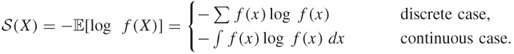
One of the most celebrated measures of uncertainty in information theory is the Shannon entropy, or simply entropy. The entropy of a discrete random variable ![]() with density
with density ![]() is defined as
is defined as
![]()
Here ![]() is interpreted as a random character from an alphabet
is interpreted as a random character from an alphabet ![]() , such that
, such that ![]() with probability
with probability ![]() . We will use the convention
. We will use the convention ![]() .
.
It can be shown that the most efficient way to transmit characters sampled from ![]() over a binary channel is to encode them such that the number of bits required to transmit
over a binary channel is to encode them such that the number of bits required to transmit ![]() is equal to
is equal to ![]() . It follows that
. It follows that ![]() is the expected bit length required to send a random character
is the expected bit length required to send a random character ![]() .
.
A more general approach, which includes continuous random variables, is to define the entropy of a random variable ![]() with density
with density ![]() by
by
Definition (A.29) can easily be extended to random vectors ![]() as (in the continuous case)
as (in the continuous case)
A.30 ![]()
Often, ![]() is called the joint entropy of the random variables
is called the joint entropy of the random variables ![]() and is also written as
and is also written as ![]() . In the continuous case,
. In the continuous case, ![]() is frequently referred to as the differential entropy to distinguish it from the discrete case.
is frequently referred to as the differential entropy to distinguish it from the discrete case.
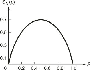
Let ![]() have a
have a ![]() distribution for some
distribution for some ![]() . The density
. The density ![]() of
of ![]() is given by
is given by ![]() and
and ![]() , so that the entropy of
, so that the entropy of ![]() is
is
![]()
The graph of the entropy as a function of ![]() is depicted in Figure A.4. Note that the entropy is maximal for
is depicted in Figure A.4. Note that the entropy is maximal for ![]() , which gives the uniform density on
, which gives the uniform density on ![]() .
.
Figure A.4 The entropy for the ![]() distribution as a function of
distribution as a function of ![]() .
.
Next, consider a sequence ![]() of iid
of iid ![]() random variables. Let
random variables. Let ![]() . The density of
. The density of ![]() , say
, say ![]() , is simply the product of the densities of the
, is simply the product of the densities of the ![]() , so that
, so that
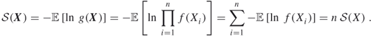
The properties of ![]() in the continuous case are somewhat different from those in the discrete one. In particular,
in the continuous case are somewhat different from those in the discrete one. In particular,
It is not difficult to see that of any density ![]() , the one that gives the maximum entropy is the uniform density on
, the one that gives the maximum entropy is the uniform density on ![]() . That is,
. That is,
A.31 ![]()
A.2.2 Kullback–Leibler Cross-Entropy
Let ![]() and
and ![]() be two densities on
be two densities on ![]() . The Kullback–Leibler cross-entropy between
. The Kullback–Leibler cross-entropy between ![]() and
and ![]() is defined (in the continuous case) as
is defined (in the continuous case) as
A.32 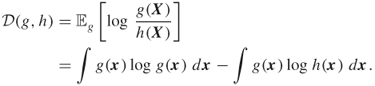
![]() is also called the Kullback–Leibler divergence, the cross-entropy, and the relative entropy. If not stated otherwise, we shall call
is also called the Kullback–Leibler divergence, the cross-entropy, and the relative entropy. If not stated otherwise, we shall call ![]() the cross-entropy between
the cross-entropy between ![]() and
and ![]() . Notice that
. Notice that ![]() is not a distance between
is not a distance between ![]() and
and ![]() in the formal sense, because, in general,
in the formal sense, because, in general, ![]() . Nonetheless, it is often useful to think of
. Nonetheless, it is often useful to think of ![]() as a distance because
as a distance because
![]()
and ![]() if and only if
if and only if ![]() . This follows from Jensen's inequality (if
. This follows from Jensen's inequality (if ![]() is a convex function, such as
is a convex function, such as ![]() , then
, then ![]() ). Namely,
). Namely,
![]()
A.3 Efficiency of Estimators
In this book, we frequently use
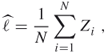
which presents an unbiased estimator of the unknown quantity ![]() , where
, where ![]() are independent replications of some random variable
are independent replications of some random variable ![]() .
.
By the central limit theorem, ![]() has approximately a
has approximately a ![]() distribution for large
distribution for large ![]() . We shall estimate
. We shall estimate ![]() via the sample variance
via the sample variance
By the law of large numbers, ![]() converges with probability 1 to
converges with probability 1 to ![]() . Consequently, for
. Consequently, for ![]() and large
and large ![]() , the approximate
, the approximate ![]() confidence interval for
confidence interval for ![]() is given by
is given by
![]()
where ![]() is the
is the ![]() quantile of the standard normal distribution. For example, for
quantile of the standard normal distribution. For example, for ![]() we have
we have ![]() . The quantity
. The quantity
![]()
is often used in the simulation literature as an accuracy measure for the estimator ![]() . For large
. For large ![]() it converges to the relative error of
it converges to the relative error of ![]() , defined as
, defined as
A.34 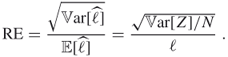
The square of the relative error
A.35 ![]()
is called the squared coefficient of variation.
Consider estimation of the tail probability ![]() of some random variable
of some random variable ![]() for a large number
for a large number ![]() . If
. If ![]() is very small, then the event
is very small, then the event ![]() is called a rare event and the probability
is called a rare event and the probability ![]() is called a rare-event probability.
is called a rare-event probability.
We may attempt to estimate ![]() via (A.33) as
via (A.33) as
which involves drawing a random sample ![]() from the pdf of
from the pdf of ![]() and defining the indicators
and defining the indicators ![]() ,
, ![]() . The estimator
. The estimator ![]() thus defined is called the crude Monte Carlo (CMC) estimator. For small
thus defined is called the crude Monte Carlo (CMC) estimator. For small ![]() the relative error of the CMC estimator is given by
the relative error of the CMC estimator is given by
A.37 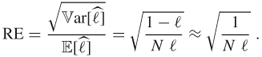
As a numerical example, suppose that ![]() . In order to estimate
. In order to estimate ![]() accurately with relative error, say,
accurately with relative error, say, ![]() , we need to choose a sample size
, we need to choose a sample size
![]()
This shows that estimating small probabilities via CMC estimators is computationally meaningless.![]()
A.3.1 Complexity
The theoretical framework in which one typically examines rare-event probability estimation is based on complexity theory (see, for example, [4]).
In particular, the estimators are classified either as polynomial-time or as exponential-time. It is shown in [4] that for an arbitrary estimator, ![]() of
of ![]() , to be polynomial-time as a function of some
, to be polynomial-time as a function of some ![]() , it suffices that its squared coefficient of variation,
, it suffices that its squared coefficient of variation, ![]() , or its relative error,
, or its relative error, ![]() , is bounded in
, is bounded in ![]() by some polynomial function,
by some polynomial function, ![]() For such polynomial-time estimators, the required sample size to achieve a fixed relative error does not grow too fast as the event becomes rarer.
For such polynomial-time estimators, the required sample size to achieve a fixed relative error does not grow too fast as the event becomes rarer.
Consider the estimator (A.36) and assume that ![]() becomes very small as
becomes very small as ![]() . Note that
. Note that
![]()
Hence, the best one can hope for with such an estimator is that its second moment of ![]() decreases proportionally to
decreases proportionally to ![]() as
as ![]() . We say that the rare-event estimator (A.36) has bounded relative error if for all
. We say that the rare-event estimator (A.36) has bounded relative error if for all ![]()
A.38 ![]()
for some fixed ![]() . Because bounded relative error is not always easy to achieve, the following weaker criterion is often used. We say that the estimator (A.36) is logarithmically efficient (sometimes called asymptotically optimal) if
. Because bounded relative error is not always easy to achieve, the following weaker criterion is often used. We say that the estimator (A.36) is logarithmically efficient (sometimes called asymptotically optimal) if
A.39 ![]()
Consider the CMC estimator (A.36). We have
![]()
so that
![]()
Hence, the CMC estimator is not logarithmically efficient, and therefore alternative estimators must be found to estimate small ![]() .
.![]()
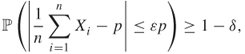
A.3.2 Complexity of Randomized Algorithms
A randomized algorithm is said to give an ![]() -approximation for a parameter
-approximation for a parameter ![]() if its output
if its output ![]() satisfies
satisfies
that is, the “relative error” ![]() of the approximation
of the approximation ![]() lies with high probability (
lies with high probability (![]() ) below some small number
) below some small number ![]() .
.
One of the main tools in proving (A.40) for various randomized algorithms is the so-called Chernoff bound, which states that for any random variable ![]() and any number
and any number ![]()
Namely, for any fixed ![]() and
and ![]() , define the functions
, define the functions ![]() and
and ![]() . Then, clearly
. Then, clearly ![]() for all
for all ![]() . As a consequence, for any
. As a consequence, for any ![]() ,
,
![]()
The bound (A.41) now follows by taking the smallest such ![]() .
.
An important application is the following.
provided ![]() .
.
For the proof see, for example, Rubinstein and Kroese [108].
Note that the sample mean in Theorem A.1 provides a FPRAS for estimating ![]() . Note also that the input vector
. Note also that the input vector ![]() consists of the Bernoulli variables
consists of the Bernoulli variables ![]() .
.
There exists a fundamental connection between the ability to sample uniformly from some set ![]() and counting the number of elements of interest. Because exact uniform sampling is not always feasible, MCMC techniques are often used to sample approximately from a uniform distribution.
and counting the number of elements of interest. Because exact uniform sampling is not always feasible, MCMC techniques are often used to sample approximately from a uniform distribution.
It is well-known [88] that the definition of variation distance coincides with that of an ![]() -uniform sample in the sense that a sampling algorithm returns an
-uniform sample in the sense that a sampling algorithm returns an ![]() -uniform sample on
-uniform sample on ![]() if and only if the variation distance between its output distribution
if and only if the variation distance between its output distribution ![]() and the uniform distribution
and the uniform distribution ![]() satisfies
satisfies
Bounding the variation distance between the uniform distribution and the empirical distribution of the Markov chain obtained after some warm-up period is a crucial issue while establishing the foundations of randomized algorithms because, with a bounded variation distance, one can produce an efficient approximation for ![]() .
.
An important issue is to prove that given an FPAUS for a combinatorial problem, one can construct a corresponding FPRAS.
An FPAUS for independent sets takes as input a graph ![]() and a parameter
and a parameter ![]() . The sample space
. The sample space ![]() consists of all independent sets in
consists of all independent sets in ![]() with the output being an
with the output being an ![]() -uniform sample from
-uniform sample from ![]() . The time to produce such an
. The time to produce such an ![]() -uniform sample should be polynomial in the size of the graph and
-uniform sample should be polynomial in the size of the graph and ![]() . Based on the product formula (4.2), Mitzenmacher and Upfal [88] prove that, given an FPAUS, one can construct a corresponding FPRAS.
. Based on the product formula (4.2), Mitzenmacher and Upfal [88] prove that, given an FPAUS, one can construct a corresponding FPRAS.![]()