Chapter 2
Cross-Entropy Method
2.1 Introduction
The cross-entropy (CE) method is a powerful technique for solving difficult estimation and optimization problems, based on Kullback-Leibler (or cross-entropy) minimization [15]. It was pioneered by Rubinstein in 1999 [100] as an adaptive importance sampling procedure for the estimation of rare-event probabilities. Subsequent work in [101] [102] has shown that many optimization problems can be translated into a rare-event estimation problem. As a result, the CE method can be utilized as randomized algorithms for optimization. The gist of the idea is that the probability of locating an optimal or near-optimal solution using naive random search is a rare event probability. The cross-entropy method can be used to gradually change the sampling distribution of the random search so that the rare event is more likely to occur. For this purpose, using the cross-entropy or Kullback-Leibler divergence as a measure of closeness between two sampling distributions, the method estimates a sequence of parametric sampling distributions that converges to a distribution with probability mass concentrated in a region of near-optimal solutions.
To date, the CE method has been successfully applied to optimization and estimation problems. The former includes mixed-integer nonlinear programming [69], continuous optimal control problems [111] [112], continuous multiextremal optimization [71], multidimensional independent component analysis [116], optimal policy search [19], clustering [11] [17, 72], signal detection [80], DNA sequence alignment [67] [93], fiber design [27], noisy optimization problems such as optimal buffer allocation [2], resource allocation in stochastic systems [31], network reliability optimization [70], vehicle routing optimization with stochastic demands [29], power system combinatorial optimization problems [45], and neural and reinforcement learning [81] [86, 118] [128]. CE has even been used as a main engine for playing games such as Tetris, Go, and backgammon [26].
In the estimation setting, the CE method can be viewed as an adaptive importance sampling procedure. In the optimization setting, the optimization problem is first translated into a rare-event estimation problem, and then the CE method for estimation is used as an adaptive algorithm to locate theoptimum.
The CE method is based on a simple iterative procedure where each iteration contains two phases: (a) generate a random data sample (trajectories, vectors, etc.) according to a specified mechanism; (b) update the parameters of the random mechanism on the basis of the data, in order to produce a “better” sample in the next iteration.
Among the two, optimization and estimation, CE is best known for optimization, for which it is able to handle problems of size up to thousands in a reasonable time limit. For estimation and also counting problems, multilevel CE can be useful only for problems of small and moderate size. The main reason for that is, unlike optimization, in estimation multilevel CE involves likelihood ratios factors for all variables. The well-known degeneracy of the likelihood ratio estimators [106] causes CE to perform poorly in high dimensions. To overcome this problem, [25] proposes a variation of the CE method by considering a single iteration for determining the importance sampling density. For this approach to work, one must be able to generate samples from the optimal (zero-variance) density.
A tutorial on the CE method is given in [37]. A comprehensive treatment can be found in [107]. The CE method website (www.cemethod.org) lists several hundred publications.
The rest of this chapter is organized as follows. Section 2.2 presents a general CE algorithm for the estimation of rare event probabilities, while Section 2.3 introduces a slight modification of this algorithm for solving combinatorial optimization problems. We consider applications of the CE method to the multidimensional knapsack problem, to the Mastermind game, and to Markov decision problems. Also, we provide supportive numerical results on the performance of the algorithm for these problems. Sections 2.4 and 2.5 discuss advanced versions of CE to deal with continuous and noisy optimization, respectively.
2.2 Estimation of Rare-Event Probabilities
Consider the problem of computing a probability of the form
for some fixed level ![]() . In this expression
. In this expression ![]() is the sample performance, and
is the sample performance, and ![]() a random vector with probability density function (pdf)
a random vector with probability density function (pdf) ![]() , sometimes called the prior pdf. The standard or crude Monte Carlo estimation method is based on repetitive sampling from
, sometimes called the prior pdf. The standard or crude Monte Carlo estimation method is based on repetitive sampling from ![]() and using the sample average:
and using the sample average:
where ![]() are independent and identically distributed (iid) samples drawn from
are independent and identically distributed (iid) samples drawn from ![]() . However, for rare-event probabilities, say
. However, for rare-event probabilities, say ![]() or less, this method fails for the following reasons [108]. The efficiency of the estimator is measured by its relative error (RE), which is defined as
or less, this method fails for the following reasons [108]. The efficiency of the estimator is measured by its relative error (RE), which is defined as
Clearly, for the standard estimator (2.2)
![]()
Thus, for small probabilities, meaning ![]() , we get
, we get
This says that the sample size ![]() is of the order
is of the order ![]() to obtain relative error of
to obtain relative error of ![]() . For rare-event probabilities, this sample size leads to unmanageable computation time. For instance, let
. For rare-event probabilities, this sample size leads to unmanageable computation time. For instance, let ![]() be the maximum number of customers that during a busy period of an
be the maximum number of customers that during a busy period of an ![]() queue is present. For a load at 80%, the probability can be computed to be
queue is present. For a load at 80%, the probability can be computed to be ![]() . A simulation to obtain relative error of 10% would require about
. A simulation to obtain relative error of 10% would require about ![]() samples of
samples of ![]() (busy cycles). On a 2.79 Ghz (0.99GB RAM) PC this would take about 18 days.
(busy cycles). On a 2.79 Ghz (0.99GB RAM) PC this would take about 18 days.
Assuming asymptotic normality of the estimator, the confidence intervals (CI) follow in a standard way. For example, a 95% CI for ![]() is given by
is given by
![]()
This shows again the reciprocal relationship between sample size and rare-event probability to obtain accuracy: suppose one wishes that the confidence half width is at most ![]() % relative to the estimate
% relative to the estimate ![]() . This boils down to
. This boils down to
![]()
For variance reduction we apply importance sampling simulation using pdf ![]() , that is, we draw independent and identically distributed samples
, that is, we draw independent and identically distributed samples ![]() from
from ![]() , calculate their likelihood ratios
, calculate their likelihood ratios
![]()
and set the importance sampling estimator by
By writing ![]() , we see that this estimator is of the form
, we see that this estimator is of the form ![]() . Again, we measure efficiency by its relative error, similar to (2.3), which might be estimated by
. Again, we measure efficiency by its relative error, similar to (2.3), which might be estimated by ![]() , with
, with
2.5 
being the sample variance of the ![]() .
.
In almost all realistic problems, the prior pdf ![]() belongs to a parameterized family
belongs to a parameterized family
2.6 ![]()
That means that ![]() is given by some fixed parameter
is given by some fixed parameter ![]() . Then it is natural to choose the importance sampling pdf
. Then it is natural to choose the importance sampling pdf ![]() from the same family using another parameter
from the same family using another parameter ![]() , or
, or ![]() , etc. In that case the likelihood ratio becomes
, etc. In that case the likelihood ratio becomes
2.7 ![]()
We refer to the original parameter ![]() as the nominal parameter of the problem, and we call parameters
as the nominal parameter of the problem, and we call parameters ![]() used in the importance sampling, the reference parameters.
used in the importance sampling, the reference parameters.
the problem is cast in the framework of (2.1). Note that we can estimate (2.1) via (2.4) by drawing ![]() independently from exponential distributions that are possibly different from the original ones. That is,
independently from exponential distributions that are possibly different from the original ones. That is, ![]() instead of
instead of ![]() ,
, ![]() .
.
The idea of the CE method is to choose the importance sampling pdf ![]() from within the parametric class of pdfs
from within the parametric class of pdfs ![]() such that the Kullback-Leibler entropy between
such that the Kullback-Leibler entropy between ![]() and the optimal (zero variance) importance sampling pdf
and the optimal (zero variance) importance sampling pdf ![]() , given by [107],
, given by [107],
![]()
is minimal. The Kullback-Leibler divergence between ![]() and
and ![]() is given by
is given by
2.8 ![]()
The CE minimization procedure then reduces to finding an optimal reference parameter, ![]() , say by cross-entropy minimization:
, say by cross-entropy minimization:
where ![]() is any reference parameter and the subscript in the expectation operator indicates the density of
is any reference parameter and the subscript in the expectation operator indicates the density of ![]() . This
. This ![]() can be estimated via the stochastic counterpart of (2.9):
can be estimated via the stochastic counterpart of (2.9):
where ![]() are drawn from
are drawn from ![]() .
.
The optimal parameter ![]() in (2.10) can often be obtained in explicit form, in particular when the class of sampling distributions forms an exponential family [[107], pages 319–320]. Indeed, analytical updating formulas can be found whenever explicit expressions for the maximal likelihood estimators of the parameters can be found [[37], page 36].
in (2.10) can often be obtained in explicit form, in particular when the class of sampling distributions forms an exponential family [[107], pages 319–320]. Indeed, analytical updating formulas can be found whenever explicit expressions for the maximal likelihood estimators of the parameters can be found [[37], page 36].
In the other cases, we consider a multilevel approach, where we generate a sequence of reference parameters ![]() and a sequence of levels
and a sequence of levels ![]() , while iterating in both
, while iterating in both ![]() and
and ![]() . Our ultimate goal is to have
. Our ultimate goal is to have ![]() close to
close to ![]() after some number of iterations and to use
after some number of iterations and to use ![]() in the importance sampling density
in the importance sampling density ![]() to estimate
to estimate ![]() .
.
We start with ![]() and choose
and choose ![]() to be a not too small number, say
to be a not too small number, say ![]() . At the first iteration, we choose
. At the first iteration, we choose ![]() to be the optimal parameter for estimating
to be the optimal parameter for estimating ![]() , where
, where ![]() is the
is the ![]() -quantile of
-quantile of ![]() . That is,
. That is, ![]() is the largest real number for which
is the largest real number for which ![]() Thus, if we simulate under
Thus, if we simulate under ![]() , then level
, then level ![]() is reached with a reasonably high probability of around
is reached with a reasonably high probability of around ![]() . In this way we can estimate the (unknown!) level
. In this way we can estimate the (unknown!) level ![]() , simply by generating a random sample
, simply by generating a random sample ![]() from
from ![]() , and calculating the
, and calculating the ![]() -quantile of the order statistics of the performances
-quantile of the order statistics of the performances ![]() ; that is, denote the ordered set of performance values by
; that is, denote the ordered set of performance values by ![]() , then
, then
![]()
where ![]() denotes the integer part. Next, the reference parameter
denotes the integer part. Next, the reference parameter ![]() can be estimated via (2.10), replacing
can be estimated via (2.10), replacing ![]() with the estimate of
with the estimate of ![]() . Note that we can use here the same sample for estimating both
. Note that we can use here the same sample for estimating both ![]() and
and ![]() . This means that
. This means that ![]() is estimated on the basis of the
is estimated on the basis of the ![]() best samples, that is, the samples
best samples, that is, the samples ![]() for which
for which ![]() is greater than or equal to
is greater than or equal to ![]() . These form the elite samples in the first iteration. We repeat these steps in the subsequent iterations. The two updating phases, starting from
. These form the elite samples in the first iteration. We repeat these steps in the subsequent iterations. The two updating phases, starting from ![]() are given below:
are given below:
The procedure terminates when at some iteration ![]() a level
a level ![]() is reached that is at least
is reached that is at least ![]() , and thus the original value of
, and thus the original value of ![]() can be used without getting too few samples. We then reset
can be used without getting too few samples. We then reset ![]() to
to ![]() , reset the corresponding elite set, and deliver the final reference parameter
, reset the corresponding elite set, and deliver the final reference parameter ![]() , using again (2.12). This
, using again (2.12). This ![]() is then used in (2.4) to estimate
is then used in (2.4) to estimate ![]() .
.
Instead of updating the parameter vector ![]() directly via (2.12), we use the following smoothed version:
directly via (2.12), we use the following smoothed version:
where ![]() is the parameter vector given in (2.12), and
is the parameter vector given in (2.12), and ![]() is called the smoothing parameter, typically with
is called the smoothing parameter, typically with ![]() . Clearly, for
. Clearly, for ![]() we have our original updating rule. The reason for using the smoothed (2.13) instead of the original updating rule is twofold: (a) to smooth out the values of
we have our original updating rule. The reason for using the smoothed (2.13) instead of the original updating rule is twofold: (a) to smooth out the values of ![]() , (b) to reduce the probability that some component
, (b) to reduce the probability that some component ![]() of
of ![]() will be zero or one at the first few iterations. This is particularly important when
will be zero or one at the first few iterations. This is particularly important when ![]() is a vector or matrix of probabilities. Because in those cases, when
is a vector or matrix of probabilities. Because in those cases, when ![]() it is always ensured that
it is always ensured that ![]() , while for
, while for ![]() one might have (even at the first iterations) that either
one might have (even at the first iterations) that either ![]() or
or ![]() for some indices
for some indices ![]() . As a result, the algorithm will converge to a wrong solution.
. As a result, the algorithm will converge to a wrong solution.
The resulting CE algorithm for rare-event probability estimation can thus be written as follows.
Apart from specifying the family of sampling pdfs, the sample sizes ![]() and
and ![]() , and the rarity parameter
, and the rarity parameter ![]() , the algorithm is completely self-tuning. The sample size
, the algorithm is completely self-tuning. The sample size ![]() for determining a good reference parameter can usually be chosen much smaller than the sample size
for determining a good reference parameter can usually be chosen much smaller than the sample size ![]() for the final importance sampling estimation, say
for the final importance sampling estimation, say ![]() versus
versus ![]() = 100,000. Under certain technical conditions [107], the deterministic version of Algorithm 2.1 is guaranteed to terminate (reach level
= 100,000. Under certain technical conditions [107], the deterministic version of Algorithm 2.1 is guaranteed to terminate (reach level ![]() ) provided that
) provided that ![]() is chosen small enough.
is chosen small enough.
Note that Algorithm 2.1 breaks down the “hard” problem of estimating the very small probability ![]() into a sequence of “simple” problems, generating a sequence of pairs
into a sequence of “simple” problems, generating a sequence of pairs ![]() , depending on
, depending on ![]() , which is called the rarity parameter. Convergence of Algorithm 2.1 is discussed in [107]. Other convergence proofs for the CE method may be found in [33] and [84].
, which is called the rarity parameter. Convergence of Algorithm 2.1 is discussed in [107]. Other convergence proofs for the CE method may be found in [33] and [84].
Optimization problems of the form (2.12) appear frequently in statistics. In particular, if the ![]() factor is omitted, which will turn out to be important in CE optimization, one can write (2.12) also as
factor is omitted, which will turn out to be important in CE optimization, one can write (2.12) also as
![]()
where the product is the joint density of the elite samples. Consequently, ![]() is chosen such that the joint density of the elite samples is maximized. Viewed as a function of the parameter
is chosen such that the joint density of the elite samples is maximized. Viewed as a function of the parameter ![]() , rather than the data
, rather than the data ![]() , this function is called the likelihood. In other words,
, this function is called the likelihood. In other words, ![]() is the maximum likelihood estimator (it maximizes the likelihood) of
is the maximum likelihood estimator (it maximizes the likelihood) of ![]() based on the elite samples. When the
based on the elite samples. When the ![]() factor is present, the form of the updating formula remains similar.
factor is present, the form of the updating formula remains similar.
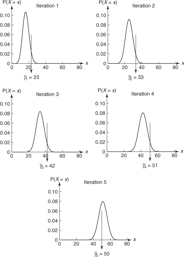
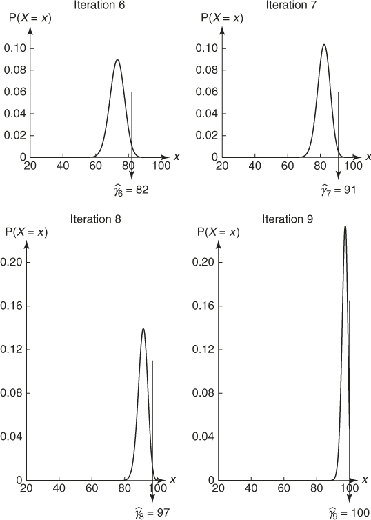
To provide further insight into Algorithm 2.1, we shall follow it step-by-step in a couple of toy examples.

is a rare-event probability. Assume further that ![]() is fixed and we want to estimate the optimal parameter
is fixed and we want to estimate the optimal parameter ![]() in
in ![]() using (2.12).
using (2.12).
where
is the likelihood ratio of the ![]() -th sample. To find the optimal
-th sample. To find the optimal ![]() , we consider the first-order condition. We obtain
, we consider the first-order condition. We obtain
In other words, ![]() is simply the sample fraction of the elite samples, weighted by the likelihood ratios. Note that, without the weights
is simply the sample fraction of the elite samples, weighted by the likelihood ratios. Note that, without the weights ![]() , we would obtain the maximum likelihood estimator of
, we would obtain the maximum likelihood estimator of ![]() for the
for the ![]() distribution based on the elite samples, in accordance with Remark 2.5. Note also that (2.14) can be viewed as a stochastic counterpart of the deterministic updating formula
distribution based on the elite samples, in accordance with Remark 2.5. Note also that (2.14) can be viewed as a stochastic counterpart of the deterministic updating formula
where ![]() is the
is the ![]() -quantile of the
-quantile of the ![]() distribution.
distribution.
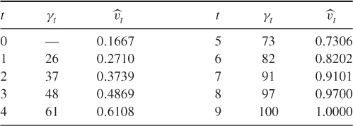
| 0 | — | 0.1667 |
| 1 | 23 | 0.2530 |
| 2 | 33 | 0.3376 |
| 3 | 42 | 0.4263 |
| 4 | 51 | 0.5124 |
| 5 | 50 | 0.5028 |
![]()
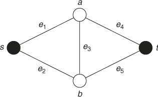
as the nominal parameter and estimate the probability ![]() that the minimum path length is greater than
that the minimum path length is greater than ![]() .
.
2.15 
2.3 Cross-Entropy Method forOptimization
Consider the following optimization problem:
having ![]() as the set of optimal solutions.
as the set of optimal solutions.
The problem is called a discrete or continuous optimization problem, depending on whether ![]() is discrete or continuous. An optimization problem where some
is discrete or continuous. An optimization problem where some ![]() are discrete and some others are continuous variables is called a mixed optimization problem. An optimization problem with a finite state space (
are discrete and some others are continuous variables is called a mixed optimization problem. An optimization problem with a finite state space (![]() ) is called a combinatorial optimization problem. The latter will be the main focus of this section.
) is called a combinatorial optimization problem. The latter will be the main focus of this section.
We will show here how the cross-entropy method can be applied for approximating a pdf ![]() that is concentrated on
that is concentrated on ![]() . In fact, the iterations of the cross-entropy algorithm generate a sequence of pdfs
. In fact, the iterations of the cross-entropy algorithm generate a sequence of pdfs ![]() associated with a sequence of decreasing sets converging to
associated with a sequence of decreasing sets converging to ![]() .
.
Suppose that we set the optimal value ![]() , then an optimal pdf
, then an optimal pdf ![]() is characterized by
is characterized by
![]()
This matches exactly to the case of degeneracy of the cross-entropy algorithm for rare-event simulation in Example 2.7.
Hence, the starting point is to associate with the optimization problem (2.16) a meaningful estimation problem. To this end, we define a collection of indicator functions ![]() on
on ![]() for various levels
for various levels ![]() . Next, let
. Next, let ![]() be a family of probability densities on
be a family of probability densities on ![]() , parameterized by real-valued parameters
, parameterized by real-valued parameters ![]() . For a fixed
. For a fixed ![]() we associate with (2.16) the problem of estimating the rare-event probability
we associate with (2.16) the problem of estimating the rare-event probability
We call the estimation problem (2.17) the associated stochastic problem.
It is important to understand that one of the main goals of CE in optimization is to generate a sequence of pdfs ![]() , converging to a pdf
, converging to a pdf ![]() that is close or equal to an optimal pdf
that is close or equal to an optimal pdf ![]() . For this purpose we apply Algorithm 2.1 for rare-event estimation, but without fixing in advance
. For this purpose we apply Algorithm 2.1 for rare-event estimation, but without fixing in advance ![]() . It is plausible that if
. It is plausible that if ![]() is close to
is close to ![]() , then
, then ![]() assigns most of its probability mass on
assigns most of its probability mass on ![]() , and thus any
, and thus any ![]() drawn from this distribution can be used as an approximation to an optimal solution
drawn from this distribution can be used as an approximation to an optimal solution ![]() , and the corresponding function value as an approximation to the true optimal
, and the corresponding function value as an approximation to the true optimal ![]() in (2.16).
in (2.16).
In summary, to solve a combinatorial optimization problem we will employ the CE Algorithm 2.1 for rare-event estimation without fixing ![]() in advance. By doing so, the CE algorithm for optimization can be viewed as a modified version of Algorithm 2.1. In particular, in analogy to Algorithm 2.1, we choose a not very small number
in advance. By doing so, the CE algorithm for optimization can be viewed as a modified version of Algorithm 2.1. In particular, in analogy to Algorithm 2.1, we choose a not very small number ![]() , say
, say ![]() , initialize the parameter
, initialize the parameter ![]() by setting
by setting ![]() , and proceed as follows:
, and proceed as follows:
Note that, in contrast to the formulas (2.11) and (2.12) (for the rare-event setting), formulas (2.19) and (2.20) do not contain the likelihood ratio factors ![]() . The reason is that in the rare-event setting, the initial (nominal) parameter
. The reason is that in the rare-event setting, the initial (nominal) parameter ![]() is specified in advance and is an essential part of the estimation problem. In contrast, the initial reference vector
is specified in advance and is an essential part of the estimation problem. In contrast, the initial reference vector ![]() in the associated stochastic problem is quite arbitrary. In effect, by dropping the likelihood ratio factor, we can efficiently estimate at each iteration
in the associated stochastic problem is quite arbitrary. In effect, by dropping the likelihood ratio factor, we can efficiently estimate at each iteration ![]() the CE optimal high-dimensional reference parameter vector
the CE optimal high-dimensional reference parameter vector ![]() for the rare event probability
for the rare event probability ![]() by avoiding the degeneracy properties of the likelihood ratio.
by avoiding the degeneracy properties of the likelihood ratio.
Thus, the main CE optimization algorithm, which includes smoothed updating of parameter vector ![]() and which presents a slight modification of Algorithm 2.1 can be summarized as follows.
and which presents a slight modification of Algorithm 2.1 can be summarized as follows.
Note that when ![]() must be minimized instead of maximized, we simply change the inequalities “
must be minimized instead of maximized, we simply change the inequalities “![]() ” to “
” to “![]() ” and take the
” and take the ![]() -quantile instead of the
-quantile instead of the ![]() -quantile. Alternatively, one can just maximize
-quantile. Alternatively, one can just maximize ![]() .
.
then stop.
As an alternative estimate for ![]() , one can consider
, one can consider
2.22 ![]()
Before one implements the algorithm, one must decide on specifying the initial vector ![]() , the sample size
, the sample size ![]() , the stopping parameter
, the stopping parameter ![]() , and the rarity parameter
, and the rarity parameter ![]() . However, the execution of the algorithm is “self-tuning.”
. However, the execution of the algorithm is “self-tuning.”
Note that the estimation Step 7 of Algorithm 2.1 is omitted in Algorithm 2.2, because, in the optimization setting, we are not interested in estimating ![]() per se.
per se.
Algorithm 2.2 can, in principle, be applied to any discrete optimization problem. However, for each individual problem, two essential ingredients need to be supplied:
In general, there are many ways to generate samples from ![]() , and it is not always immediately clear which way of generating the sample will yield better results or easier updating formulas.
, and it is not always immediately clear which way of generating the sample will yield better results or easier updating formulas.
Below we present several applications of the CE method to combinatorial optimization problems, namely to the multidimensional 0/1 knapsack problem, the mastermind game, and to reinforcement learning in Markov decision problems. We demonstrate numerically the efficiency of the CE method and its fast convergence for several case studies. For additional applications of CE, see [107].
2.3.1 The Multidimensional 0/1 Knapsack Problem
Consider the multidimensional 0/1 knapsack problem (see Section A.1.2):
In other words, the goal is to maximize the performance function ![]()
![]() over the set
over the set ![]() given by the knapsack constraints of (2.23).
given by the knapsack constraints of (2.23).
Note that each item ![]() is either chosen,
is either chosen, ![]() , or left out,
, or left out, ![]() . We model this by a Bernoulli random variable
. We model this by a Bernoulli random variable ![]() , with parameter
, with parameter ![]() . By setting these variables independent, we get the following parameterized set:
. By setting these variables independent, we get the following parameterized set:
of Bernoulli pdfs. The optimal solution ![]() of the knapsack problem (2.23) is characterized by a degenerate pdf
of the knapsack problem (2.23) is characterized by a degenerate pdf ![]() for which all
for which all ![]() ; that is,
; that is,
![]()
To proceed, consider the stochastic program 2.20. We have
where, for convenience, we write ![]() . Applying the first-order optimality conditions we have
. Applying the first-order optimality conditions we have
for ![]() .
.
As a concrete example, consider the knapsack problem; available at http://people.brunel.ac.uk/∼mastjjb/jeb/orlib/mknapinfo.html from the OR Library involving ![]() variables and
variables and ![]() constraints. In this problem the vector
constraints. In this problem the vector ![]() is
is
![]()
and the matrix ![]() and the vector
and the vector ![]() are
are
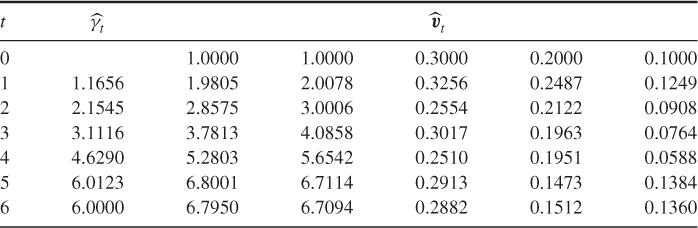
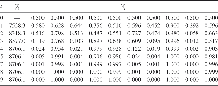
The performance of the CE algorithm is illustrated in Table 2.4 using the sample size ![]() , rarity parameter
, rarity parameter ![]() , and smoothing parameter
, and smoothing parameter ![]() . The initial probabilities were all set to
. The initial probabilities were all set to ![]() . Observe that the probability vector
. Observe that the probability vector ![]() quickly converges to a degenerate one, corresponding to the solution
quickly converges to a degenerate one, corresponding to the solution ![]() with value
with value ![]() , which is also the optimal known value
, which is also the optimal known value ![]() . Hence, the optimal solution has been found.
. Hence, the optimal solution has been found.
Table 2.4 The evolution of ![]() and
and ![]() for the
for the ![]() -Knapsack Example, using
-Knapsack Example, using ![]() ,
, ![]() , and
, and ![]() samples
samples
2.3.2 Mastermind Game
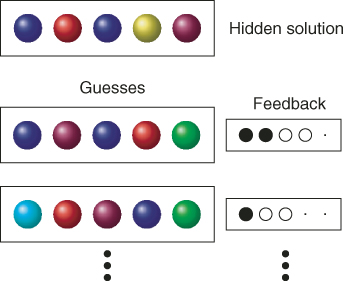
In the well-known game Mastermind, the objective is to decipher a hidden “code” of colored pegs through a series of guesses. After each guess, new information on the true code is provided in the form of black and white pegs. A black peg is earned for each peg that is exactly right and a white peg for each peg that is in the solution, but in the wrong position; see Figure 2.4. To get a feel for the game, one can visit www.archimedes-lab.org/mastermind.html and play the game.
Figure 2.4 The Mastermind game.
Consider a Mastermind game with ![]() colors, numbered
colors, numbered ![]() and
and ![]() pegs (positions). The hidden solution and a guess can be represented by a row vector of length
pegs (positions). The hidden solution and a guess can be represented by a row vector of length ![]() with numbers in
with numbers in ![]() . For example, for
. For example, for ![]() and
and ![]() the solution could be
the solution could be ![]() , and a possible guess
, and a possible guess ![]() . Let
. Let ![]() be the space of all possible guesses; clearly
be the space of all possible guesses; clearly ![]() . On
. On ![]() we define a performance function
we define a performance function ![]() that returns for each guess
that returns for each guess ![]() the “pegscore”
the “pegscore”
where ![]() and
and ![]() are the number of black and white pegs returned after the guess,
are the number of black and white pegs returned after the guess, ![]() . We have assumed, somewhat arbitrarily, that a black peg is worth twice as much as a white peg. As an example, for the solution
. We have assumed, somewhat arbitrarily, that a black peg is worth twice as much as a white peg. As an example, for the solution ![]() and guess
and guess ![]() above one gets two black pegs (for the first and third pegs in the guess) and two white pegs (for the second and fourth pegs in the guess, which match the fifth and second pegs of the solution but are in the wrong place). Hence the score for this guess is 6.
above one gets two black pegs (for the first and third pegs in the guess) and two white pegs (for the second and fourth pegs in the guess, which match the fifth and second pegs of the solution but are in the wrong place). Hence the score for this guess is 6.
There are some specially designed algorithms that efficiently solve the problem for different number of colors and pegs. For examples, see www.mathworks.com/contest/mastermind.cgi/home.html.
Note that, with the above performance function, the problem can be formulated as an optimization problem, that is, as ![]() , and hence we could apply the CE method to solve it. In order to apply the CE method we first need to generate random guesses
, and hence we could apply the CE method to solve it. In order to apply the CE method we first need to generate random guesses ![]() using an
using an ![]() probability matrix
probability matrix ![]() . Each element
. Each element ![]() of
of ![]() describes the probability that we choose the
describes the probability that we choose the ![]() th color for the
th color for the ![]() th peg (location). Since only one color may be assigned to one peg, we have that
th peg (location). Since only one color may be assigned to one peg, we have that
2.25 
In each stage ![]() of the CE algorithm, we sample independently for each row (that is, each peg) a color using a probability matrix
of the CE algorithm, we sample independently for each row (that is, each peg) a color using a probability matrix ![]() and calculate the score
and calculate the score ![]() according to (2.24). The updating of the elements
according to (2.24). The updating of the elements ![]() of the probability matrix
of the probability matrix ![]() is performed according to
is performed according to
where the samples ![]() are drawn independently and identically distributed using matrix
are drawn independently and identically distributed using matrix ![]() . Note that in this case
. Note that in this case ![]() in (2.26) simply counts the fraction of times among the elites that color
in (2.26) simply counts the fraction of times among the elites that color ![]() has been assigned to peg
has been assigned to peg ![]() .
.
2.3.2.1 Simulation Results
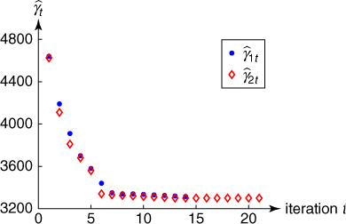
Table 2.5 represents the dynamics of the CE algorithm for the Mastermind test problem denoted at www.mathworks.com/contest/mastermind.cgi/home.html as “problem (5.2.3)” with the matrix ![]() of size
of size ![]() . We used
. We used ![]() ,
, ![]() , and
, and ![]() . It took 34 seconds of CPU time to find the true solution.
. It took 34 seconds of CPU time to find the true solution.
Table 2.5 Dynamics of Algorithm 2.2 for the mastermind problem with ![]() colors and
colors and ![]() pegs. In each iteration
pegs. In each iteration ![]() was the sampled maximal score
was the sampled maximal score
| 1 | 31 | 26 |
| 2 | 34 | 28 |
| 3 | 38 | 32 |
| 4 | 42 | 35 |
| 5 | 48 | 40 |
| 6 | 55 | 45 |
| 7 | 60 | 51 |
| 8 | 64 | 57 |
| 9 | 70 | 63 |
| 10 | 72 | 68 |
| 11 | 72 | 72 |
2.3.3 Markov Decision Process and Reinforcement Learning
The Markov decision process (MDP) model is standard in machine learning, operations research, and related fields. The application to reinforcement learning in this section is based on [83]. We start by reviewing briefly some of the basic definitions and concepts in MDP. For details see, for example, [95].
An MDP is defined by a tuple ![]() where
where
At each time instance ![]() , the decision maker observes the current state
, the decision maker observes the current state ![]() and determines the action to be taken (say
and determines the action to be taken (say ![]() ). As a result, a reward given by
). As a result, a reward given by ![]() is received immediately, and a new state
is received immediately, and a new state ![]() is chosen according to
is chosen according to ![]() . A policy or strategy
. A policy or strategy ![]() is a rule that determines, for each history
is a rule that determines, for each history ![]() of states and actions, the probability distribution of the decision maker's actions at time
of states and actions, the probability distribution of the decision maker's actions at time ![]() . A policy is called Markov if each action depends only on the current state
. A policy is called Markov if each action depends only on the current state ![]() . A Markov policy is called stationary if it does not depend on the time
. A Markov policy is called stationary if it does not depend on the time ![]() . If the decision rule
. If the decision rule ![]() of a stationary policy is nonrandomized, we say that the policy is deterministic.
of a stationary policy is nonrandomized, we say that the policy is deterministic.
In the sequel, we consider problems for which an optimal policy belongs to the class of stationary Markov policies. Associated with such a MDP are the stochastic processes of consecutive observed states ![]() and actions
and actions ![]() . For stationary policies we may denote
. For stationary policies we may denote ![]() , which is a random variable on the action set
, which is a random variable on the action set ![]() . In case of deterministic policies it degenerates in a single action. Finally, we denote the immediate rewards in state
. In case of deterministic policies it degenerates in a single action. Finally, we denote the immediate rewards in state ![]() by
by ![]() .
.
The goal of the decision maker is to maximize a certain reward function. The following are standard reward criteria:
2.28 
Suppose that the MDP is identified; that is, the transition probabilities and the immediate rewards are specified and known. Then it is well known that there exists a deterministic stationary optimal strategy for the above three cases. Moreover, there are several efficient methods for finding it, such as value iteration and policy iteration [95].
In the next section, we will restrict our attention to the stochastic shortest path MDP, where it is assumed that the process starts from a specific initial state ![]() and terminates in an absorbing state
and terminates in an absorbing state ![]() with zero reward. For the finite horizon reward criterion
with zero reward. For the finite horizon reward criterion ![]() is the time at which
is the time at which ![]() is reached (which we will assume will always happen eventually). It is well known that for the shortest path MDPthere exists a stationary Markov policy that maximizes
is reached (which we will assume will always happen eventually). It is well known that for the shortest path MDPthere exists a stationary Markov policy that maximizes ![]() for each of the reward functions above.
for each of the reward functions above.
However, when the transition probability or the reward in an MDP are unknown, the problem is much more difficult and is referred to as a learning probability. A well-known framework for learning algorithms is reinforcement learning (RL), where an agent learns the behavior of the system through trial-and-error with an unknown dynamic environment; see [61].
There are several approaches to RL, which can be roughly divided into the following three classes: model-based, model-free, and policy search. In the model-based approach, a model of the environment is first constructed. The estimated MDP is then solved using standard tools of dynamic programming (see [66]).
In the model-free approach, one learns a utility function instead of learning the model. The optimal policy is to choose at each state an action that maximizes the expected utility. The popular Q-learning algorithm (e.g., [125]) is an example of this approach.
In the policy search approach, a subspace of the policy space is searched, and the performance of policies is evaluated based on their empirical performance (e.g., [7]). An example of a gradient-based policy search method is the REINFORCE algorithm of [127]. For a direct search in the policy space approach see [98]. The CE algorithm in the next section belongs to the policy search approach.
where ![]() is a positive sequence satisfying
is a positive sequence satisfying
2.29 
2.3.3.1 Policy Learning via the CE Method
We consider a CE learning algorithm for the shortest path MDP, where it is assumed that the process starts from a specific initial state ![]() , and that there is an absorbing state
, and that there is an absorbing state ![]() with zero reward. The objective is given in (2.27), with
with zero reward. The objective is given in (2.27), with ![]() being the stopping time at which
being the stopping time at which ![]() is reached (which we will assume will always happen).
is reached (which we will assume will always happen).
To put this problem in the CE framework, consider the maximization problem (2.27). Recall that for the shortest path MDP an optimal stationary strategy exists. We can represent each stationary strategy as a vector ![]() with
with ![]() being the action taken when visiting state
being the action taken when visiting state ![]() . Writing the expectation in (2.27) as
. Writing the expectation in (2.27) as
2.30 
we see that the optimization problem (2.27) is of the form ![]() . We shall also consider the case where
. We shall also consider the case where ![]() is measured (observed) with some noise, in which case we have a noisy optimization problem.
is measured (observed) with some noise, in which case we have a noisy optimization problem.
The idea now is to combine the random policy generation and the random trajectory generation in the following way: At each stage of the CE algorithm we generate random policies and random trajectories using an auxiliary ![]() matrix
matrix ![]() , such that for each state
, such that for each state ![]() we choose action
we choose action ![]() with probability
with probability ![]() . Once this “policy matrix”
. Once this “policy matrix” ![]() is defined, each iteration of the CE algorithm comprises the following two standard phases:
is defined, each iteration of the CE algorithm comprises the following two standard phases:
The matrix ![]() is typically initialized to a uniform matrix (
is typically initialized to a uniform matrix (![]() .) We describe both the trajectory generation and updating procedure in more detail. We shall show that in calculating the associated sample performance, one can take into account the Markovian nature of the problem and speed up the Monte Carlo process.
.) We describe both the trajectory generation and updating procedure in more detail. We shall show that in calculating the associated sample performance, one can take into account the Markovian nature of the problem and speed up the Monte Carlo process.
2.3.3.2 Generating Random Trajectories
Generation of random trajectories for MDP is straightforward and is given for convenience only. All one has to do is to start the trajectory from the initial state ![]() and follow the trajectory by generating at each new state according to the probability distribution of
and follow the trajectory by generating at each new state according to the probability distribution of ![]() , until the absorbing state
, until the absorbing state ![]() is reached at, say, time
is reached at, say, time ![]() ,
,
2.3.3.3 Updating Rules
Let the ![]() trajectories
trajectories ![]() , their scores,
, their scores, ![]()
![]() , and the associated
, and the associated ![]() -quantile
-quantile ![]() of their order statistics be given. Then one can update the parameter matrix
of their order statistics be given. Then one can update the parameter matrix ![]() using the CE method, namely as per
using the CE method, namely as per
where the event ![]() means that the trajectory
means that the trajectory ![]() contains a visit to state
contains a visit to state ![]() and the event
and the event ![]() means the trajectory corresponding to policy
means the trajectory corresponding to policy ![]() contains a visit to state
contains a visit to state ![]() in which action
in which action ![]() was taken.
was taken.
We now explain how to take advantage of the Markovian nature of the problem. Let us think of a maze where a certain trajectory starts badly, that is, the path is not efficient in the beginning, but after some time it starts moving quickly toward, the goal. According to (2.32), all the updates are performed in a similar manner in every state in the trajectory. However, the actions taken in the states that were sampled near the target were successful, so one would like to “encourage” these actions. Using the Markovian property one can substantially improve the above algorithm by considering for each state the part of the reward from the visit to that state onward. We therefore use the same trajectory and simultaneously calculate the performance for every state in the trajectory separately. The idea is that each choice of action in a given state affects the reward from that point on, regardless of the past.
The sampling Algorithm 2.3 does not change in steps 1 and 2. The difference is in step 3. Given a policy ![]() and trajectory
and trajectory ![]() , we calculate the performance from every state until termination. For every state
, we calculate the performance from every state until termination. For every state ![]() in the trajectory, the (estimated) performance is
in the trajectory, the (estimated) performance is ![]() . The updating formula for
. The updating formula for ![]() is similar to (2.32), however, each state
is similar to (2.32), however, each state ![]() is updated separately according to the (estimated) performance
is updated separately according to the (estimated) performance ![]() obtained from state
obtained from state ![]() onward.
onward.
It is important to understand here that, in contrast to (2.32), the CE optimization is carried for every state separately and a different threshold parameter ![]() is used for every state
is used for every state ![]() , at iteration
, at iteration ![]() . This facilitates faster convergence for “easy” states where the optimal strategy is easy to find. The above trajectory sampling method can be viewed as a variance reduction method. Numerical results indicate that the CE algorithm with updating (2.33) is much faster than that with updating (2.32).
. This facilitates faster convergence for “easy” states where the optimal strategy is easy to find. The above trajectory sampling method can be viewed as a variance reduction method. Numerical results indicate that the CE algorithm with updating (2.33) is much faster than that with updating (2.32).
2.3.3.4 Numerical Results with the Maze Problem
The CE Algorithm with the updating rule (2.33) and trajectory generation according to Algorithm 2.3 was tested for a stochastic shortest path MDP and, in particular, for a maze problem, which presents a two-dimensional grid world. The agent moves on a grid in four possible directions. The goal of the agent is to move from the upper-left corner (the starting state) to the lower-right corner (the goal) in the shortest path possible. The maze contains obstacles (walls) into which movement is not allowed. These are modeled as forbidden moves for the agent.
We assume the following:
In addition, we introduce the following:
- A small (failure) probability not to succeed moving in an allowed direction
- A small probability of succeeding moving in the forbidden direction (“moving through the wall”)
In Figure 2.5 we present the results for ![]() maze. We set the following parameters:
maze. We set the following parameters: ![]() ,
, ![]() ,
, ![]() .
.
Figure 2.5 Performance of the CE Algorithm for the ![]() maze. Each arrow indicates a probability
maze. Each arrow indicates a probability ![]() of going in that direction.
of going in that direction.
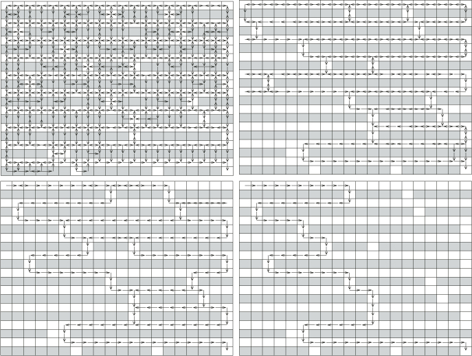
The initial policy was a uniformly random one. The success probabilities in the allowed and forbidden states were taken to be 0.95 and 0.05, respectively. The arrows ![]() in Figure 2.5 indicate that at the current iteration the probability of going from
in Figure 2.5 indicate that at the current iteration the probability of going from ![]() to
to ![]() is at least 0.01. In other words, if
is at least 0.01. In other words, if ![]() corresponds to the action that will lead to state
corresponds to the action that will lead to state ![]() from
from ![]() then we will plot an arrow from
then we will plot an arrow from ![]() to
to ![]() provided
provided ![]() .
.
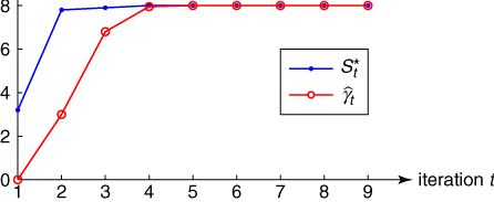
In all our experiments, CE found the target exactly, within 5–10 iterations, and CPU time was less than one minute (on a 500MHz Pentium processor). Note that the successive iterations of the policy in Figure 2.5 quickly converge to the optimal policy. We have also run the algorithm for several other mazes and the optimal policy was always found.
2.4 Continuous Optimization
When the state space is continuous, in particular, when ![]() , the optimization problem (2.16) is often referred to as a continuous optimization problem. The CE sampling distribution on
, the optimization problem (2.16) is often referred to as a continuous optimization problem. The CE sampling distribution on ![]() can be quite arbitrary and does not need to be related to the function that is being optimized. The generation of a random vector
can be quite arbitrary and does not need to be related to the function that is being optimized. The generation of a random vector ![]() in Step 2 of Algorithm 2.2 is most easily performed by drawing the
in Step 2 of Algorithm 2.2 is most easily performed by drawing the ![]() coordinates independently from some two-parameter distribution. In most applications a normal (Gaussian) distribution is employed for each component. Thus, the sampling density
coordinates independently from some two-parameter distribution. In most applications a normal (Gaussian) distribution is employed for each component. Thus, the sampling density ![]() of
of ![]() is characterized by a vector of means
is characterized by a vector of means ![]() and a vector of variances
and a vector of variances ![]() (and we may write
(and we may write ![]() ). The choice of the normal distribution is motivated by the availability of fast normal random number generators on modern statistical software and the fact that the cross-entropy minimization yields a very simple solution—at each iteration of the CE algorithm the parameter vectors
). The choice of the normal distribution is motivated by the availability of fast normal random number generators on modern statistical software and the fact that the cross-entropy minimization yields a very simple solution—at each iteration of the CE algorithm the parameter vectors ![]() and
and ![]() are the vectors of sample means and sample variance of the elements of the set of
are the vectors of sample means and sample variance of the elements of the set of ![]() best-performing vectors (that is, the elite set); see, for example, [71]. In summary, the CE method for continuous optimization with a Gaussian sampling density is as follows.
best-performing vectors (that is, the elite set); see, for example, [71]. In summary, the CE method for continuous optimization with a Gaussian sampling density is as follows.
2.34 ![]()
2.36 ![]()
Smoothing, as in Step 5, is often crucial to prevent premature shrinking of the sampling distribution. Instead of using a single smoothing factor, it is often useful to use separate smoothing factors for ![]() and
and ![]() (see (2.35)). In particular, it is suggested in [108] to use the following dynamic smoothing for
(see (2.35)). In particular, it is suggested in [108] to use the following dynamic smoothing for ![]() :
:
2.37 ![]()
where ![]() is an integer (typically between 5 and 10) and
is an integer (typically between 5 and 10) and ![]() is a smoothing constant (typically between 0.8 and 0.99). Finally, significant speed-up, can be achieved by using a parallel implementation of CE [46].
is a smoothing constant (typically between 0.8 and 0.99). Finally, significant speed-up, can be achieved by using a parallel implementation of CE [46].
Another approach is to inject extra variance into the sampling distribution, for example, by increasing the components of ![]() , once the distribution has degenerated; see the examples below and [11].
, once the distribution has degenerated; see the examples below and [11].
has various local maxima. In this case, implementing the CE Algorithm 2.4 we found that the global maximum of this function is approximately ![]() and is attained at
and is attained at ![]() . The choice of the initial value for
. The choice of the initial value for ![]() is not important, but the initial standard deviations should be chosen large enough to ensure initially a “uniform” sampling of the region of interest. The CE algorithm is stopped when all standard deviations of the sampling distribution are less than some small
is not important, but the initial standard deviations should be chosen large enough to ensure initially a “uniform” sampling of the region of interest. The CE algorithm is stopped when all standard deviations of the sampling distribution are less than some small ![]() .
.
2.5 Noisy Optimization
One of the distinguishing features of the CE Algorithm 2.2 is that it can easily handle noisy optimization problems, that is, when the objective function ![]() is corrupted with noise. We denote such noisy function as
is corrupted with noise. We denote such noisy function as ![]() and assume that for each
and assume that for each ![]() we can readily obtain an outcome of
we can readily obtain an outcome of ![]() , for example, via generation of some additional random vector
, for example, via generation of some additional random vector ![]() , whose distribution may depend on
, whose distribution may depend on ![]() .
.
A classical example of noisy optimization is simulation-based optimization [107]. A typical instance is the buffer allocation problem (BAP). The objective in the BAP is to allocate ![]() buffer spaces among the
buffer spaces among the ![]() “niches” (storage areas) between
“niches” (storage areas) between ![]() machines in a serial production line, so as to optimize some performance measure, such as the steady-state throughput. This performance measure is typically not available analytically and thus must be estimated via simulation. A detailed description of the BAP with application of CE is given in [107].
machines in a serial production line, so as to optimize some performance measure, such as the steady-state throughput. This performance measure is typically not available analytically and thus must be estimated via simulation. A detailed description of the BAP with application of CE is given in [107].
Another example is the noisy traveling salesman problem (TSP), where, say, the cost matrix ![]() , denoted now by
, denoted now by ![]() , is random. Think of
, is random. Think of ![]() as the “random” time to travel from city
as the “random” time to travel from city ![]() to city
to city ![]() .
.
The total cost of a tour ![]() is given by
is given by
We assume that ![]() .
.
The main CE optimization Algorithm 2.2 for deterministic functions ![]() is valid also for noisy ones
is valid also for noisy ones ![]() . Extensive numerical studies [107] with such noisy Algorithm 2.2 show that it works nicely because, during the course of optimization, it filters out efficiently the noise component from
. Extensive numerical studies [107] with such noisy Algorithm 2.2 show that it works nicely because, during the course of optimization, it filters out efficiently the noise component from ![]() .
.
We applied our CE Algorithm 2.2 to both deterministic and noisy TSP. We selected a number of benchmark problems from the TSP library (www.iwr.uni-heidelberg.de/groups/comopt/software/TSPLIB95/tsp/). In all cases, the same set of CE parameters were chosen: ![]() ,
, ![]() ,
, ![]() . Table 2.6 presents the performance of the deterministic version of Algorithm 2.2 for several TSPs from this library. To study the variability in the solutions, each problem was repeated 10 times. In Table 2.6, “min”, “mean”, and “max” denote the smallest (that is, best), average, and largest of the 10 estimates for the optimal value. The best-known solution is denoted by
. Table 2.6 presents the performance of the deterministic version of Algorithm 2.2 for several TSPs from this library. To study the variability in the solutions, each problem was repeated 10 times. In Table 2.6, “min”, “mean”, and “max” denote the smallest (that is, best), average, and largest of the 10 estimates for the optimal value. The best-known solution is denoted by ![]() .
.
Table 2.6 Case studies for the TSP
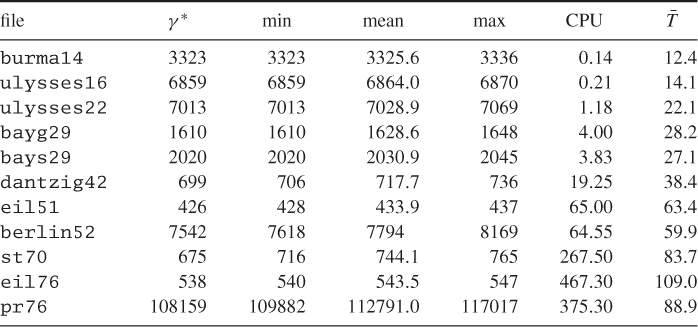
The average CPU time in seconds and the average number of iterations are given in the last two columns. The size of the problem (number of nodes) is indicated in its name. For example, st70 has ![]() nodes.
nodes.
2.39 
where ![]() is fixed, say
is fixed, say ![]() . Define next
. Define next
2.40 ![]()
and
2.41 ![]()
respectively, where ![]() is fixed, say
is fixed, say ![]() . Clearly, for
. Clearly, for ![]() and moderate
and moderate ![]() and
and ![]() , we may expect that
, we may expect that ![]() , provided the variance of
, provided the variance of ![]() is bounded.
is bounded.
2.42 ![]()
where ![]() and
and ![]() are fixed and
are fixed and ![]() is a small number, say
is a small number, say ![]() .
.