Chapter 3

Minimum Cross-Entropy Method

This chapter deals with the minimum cross-entropy method, also known as the MinxEnt method for combinatorial optimization problems and rare-event probability estimation. The main idea of MinxEnt is to associate with each original optimization problem an auxiliary single-constrained convex optimization program in terms of probability density functions. The beauty is that this auxiliary program has a closed-form solution, which becomes the optimal zero variance solution, provided the “temperature” parameter is set to minus infinity. In addition, the associated pdf based on the product of marginals obtained from the joint optimal zero variance pdf coincide with the parametric pdf of the cross-entropy (CE) method. Thus, we obtain a strong connection between CE and MinxEnt, providing solid mathematical foundations.

3.1 Introduction

Let be a continuous function defined on some closed bounded -dimensional domain . Assume that is a unique minimum point over . The following theorem is due to Pincus [94].

Let be a real-valued continuous function over closed bounded -dimensional domain . Further assume that there is a unique minimum point over at which attains (there is no restriction on the number of local minima). Then the coordinates of of are given by

3.1

The proof of the theorem is based on Laplace's formula, which for sufficiently large can be written as

This is because, for large , the major contribution to the integrals appearing in (3.1) comes from a small neighborhood of the minimizer .

Pincus' theorem holds for discrete optimization as well (assuming ). In this case, the integrals should be replaced by the relevant sums.

There are many Monte Carlo methods for evaluating the coordinates of , that is, for approximating the ratio appearing in (3.1). Among them is the celebrated simulated annealing method, which is based on a Markov chain Monte Carlo technique, also called Metropolis' sampling procedure. The idea of the method is to sample from the Boltzmann density

3.2

without resorting to calculation of the integral (the denumerator). For details see [108].

It is important to note that, in general, sampling from the complex multidimensional pdf is a formidable task. If, however, the function is separable, that is, it can be represented by

then the pdf in (3.2) decomposes as the product of its marginal pdfs, that is, it can be written as

3.3

Clearly, for a decomposable function sampling from the one-dimensional marginal pdfs of is fast.

Consider the application of the simulated annealing method to combinatorial optimization problems. As an example, consider the traveling salesman problem with cities. In this case, [1] shows how simulated annealing runs a Markov chain with states and denoting the length of the tour. As the stationary distribution of will become a degenerated one, that is, it converges to the optimal solution (shortest tour in the case of traveling salesman problem). It can be proved [1] that, in the case of multiple solutions, say solutions, we have that as the stationary distribution of will be uniform on the set of the optimal solutions.

The main drawback of simulated annealing is that it is slow and , called the annealing temperature, must be chosen heuristically.

We present a different Monte Carlo method, which we call MinxEnt. It is also associated with the Boltzmann distribution, however, it is obtained by solving a MinxEnt program of a special type and is suitable for rare-event probability estimation and approximation of the optimal solutions of a broad class of NP-hard linear integer and combinatorial optimization problems.

The main idea of the MinxEnt approach is to associate with each original optimization problem an auxiliary single-constrained convex MinxEnt program of a special type, which has a closed form solution.

The rest of this chapter is organized as follows. In Section 3.2, we present some background on the classic MinxEnt program. In Section 3.3, we establish connections between rare-event probability estimation and MinxEnt, and present what is called the basic MinxEnt (BME). Section 3.4 presents a new MinxEnt method, which involves indicator functions and is called the indicator MinxEnt (IME). We prove that the optimal pdf obtained from the solution of the IME program is a zero variance one, provided the temperature parameter is set to minus infinity. This is quite a remarkable result. In addition, we prove that the parametric pdf based on the product of marginals obtained from the optimal zero-variance pdf coincides with the parametric pdf of the standard CE method, which we covered in the previous chapter. A remarkable consequence is that we obtain a strong mathematical foundation for CE. In Section 3.5 we present the IME algorithm for optimization.

3.2 Classic MinxEnt Method

The classic MinxEnt program reads as

3.4

Here, and are -dimensional pdfs; are given functions; and is an -dimensional vector. Here, is assumed to be known and is called the prior pdf. The program (3.4) is called the classic minimum cross-entropy or simply the MinxEnt program. If the prior is constant, then , so that the minimization of in (3.4) can be replaced with the maximization of

3.5

where is the Shannon entropy [63]. The corresponding program is called the Jaynes' MinxEnt program. Note that the former minimizes the Kullback-Leibler cross-entropy, while the latter maximizes the Shannon entropy [63]. For a good paper on the generalization of MinxEnt, see [16].

The MinxEnt program, which under mild conditions [8] presents a convex constrained functional optimization problem, can be solved via Lagrange multipliers. The solution is given by [8]

3.6

where are obtained from the solution of the following system of equations:

3.7

The MinxEnt solution can be written as

3.8

where

3.9

is the normalization constant.

In the particular case where each is coordinate-wise separable, that is,

3.10

and the components of the random vector are independent. The joint pdf in (3.6) reduces to the product of marginal pdfs. In such case, we say that is decomposable.

In particular, the -th component of can be written as

3.11

3.12

coincides with the celebrated optimal exponential change of measure (ECM). Note that typically in a multidimensional ECM, one twists each component separately, using possibly different twisting parameters. In contrast, the optimal solution to the MinxEnt program is parameterized by a single-dimensional parameter , so for the multidimensional case ECM differs from MinxEnt.

To obtain better insight into the MinxEnt program, consider a particular case of (3.12) associated with die tossing. We assume and is a given discrete distribution (the prior) over the six faces of the die, where denotes the nominal parameter vector. We restrict to densities that are parameterized in this way; that is, with for all , such that . Then we denote the Kullback-Leibler cross-entropy by , which stands for . Similarly, the Shannon entropy is abbreviated to .

3.13

The optimal parameter vector , derived from the solution of (3.13), can be written component-wise as

3.14

where is derived from the numerical solution of

3.15

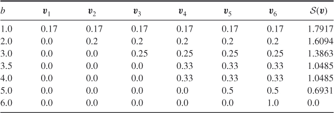
Table 3.1, which is an exact replica of Table 4.1 of [63], presents , , and the entropy as functions of for a fair die, that is, with the prior . The table is self-explanatory.

Table 3.1 , , and as Function of for a Fair Die

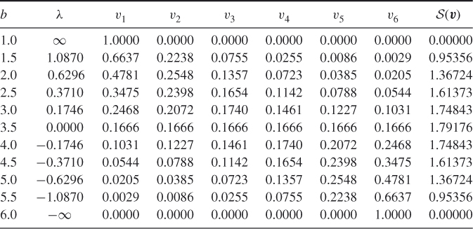
• If , then and, thus, .
• is strictly concave in and the maximal entropy .
• For the extreme values of , that is, for and , the corresponding optimal solutions are and , respectively; that is, the pdf becomes degenerated. For these cases:
  1. The entropy is , and thus there is no uncertainty (for both degenerated vectors, and ).

  2. For and we have that and , respectively. This important observation is in the spirit of Pincus [94] Theorem 3.1 and will play an important role below.

  3. It can also be readily shown that is degenerated regardless of the prior .

The above observations for the die example can be readily extended to the case where instead of one considers with and with arbitrary 's.

Taking into account that MaxEnt (with the objective function , see (3.5)) can be viewed as a particular case of MinxEnt with constant prior , we can rewrite the basic MinxEnt formulas (3.6) and (3.7) as

3.16

where are obtained from the solution of the following system of equations:

3.17

We extend next the MinxEnt program (3.4) to both equality and inequality constraints; that is, we consider the following general MinxEnt program:

3.18

In this case, applying the Kuhn-Tucker [75] conditions to the program (3.18) we readily obtain that remains the same as in (3.6), while are found from the solution of the following convex program:

3.19

3.3 Rare Events and MinxEnt

To establish the connection between MinxEnt and rare events, we consider the problem of computing a rare-event probability of the form

3.20

Here, is a random vector with pdf , is a performance function, and is such that is a rare event.

Suppose that we estimate by the importance sampling estimator

3.21

using the importance sampling pdf (see Section 2.2). Then the MinxEnt program that determines has the following single-constrained formulation:

3.22

The solution is (cf. (3.6))

3.23

and solves

3.24

We call (3.22) and (3.23), (3.24) the basic MinxEnt (BME) program and solution, respectively. This is the nonparametric setting in which generally the solution is a difficult pdf to generate samples from. As a typical example, suppose that the prior is the uniform pdf on a bounded state space , that is , where denotes the total area of the set . The rare event is . The importance sampling estimator (3.21) using the MinxEnt solution (3.23) becomes

where is a random sample from .

We give two simple examples; the first one leads to a simple simulation procedure from , the second one does not.

Suppose that , , and . In this case on , and

where and are independent uniform random variables. Thus,

The parameter solves

This is easily solved numerically for any given . The importance sampling pdf becomes

on , otherwise . Hence, under the importance sampling pdf , and are again independent but have a conditional exponential distribution with parameter , conditioned on . Generating samples from is straightforward.

Suppose that , , and . Thus, on , and

where is the circle segment above the chord . Clearly, when . Note that and are dependent. Generating samples from is easy and can be done, for example, by acceptance-rejection from uniform samples in the square . In this example we get explicit expressions neither for the normalizing constant nor for the importance sampling pdf .

As we already mentioned in Chapter 2, the cross-entropy method assumes that the prior pdf belongs to a parameterized family of pdfs (2.6), where is called the nominal parameter vector. The solution to the MinxEnt program as given in (3.23) is generally not a pdf in that parameterized family. In some cases it is possible to find an approximate pdf as in the following setting.

We say that the parameterized family of pdfs satisfies marginal expectation parameterization when

Let be the prior pdf. The MinxEnt solution for is

3.25

Suppose that the family satisfies the marginal expectation parameterization, and let be any parameter vector for the family . Then the above analysis suggests carrying out the importance sampling using equal to given in (3.25). Hence, we approximate the MinxEnt solution by with

3.26

Note that formula (3.26) is similar to the corresponding cross-entropy solution [107]

3.27

with one main difference: the indicator function in the CE formula is replaced by .

Let , and suppose that is a binary random vector with independent components and probabilities

In other words,

Assume further that the performance function is , and we want to find the optimal parameter to calculate the probability of the event .

Because is decomposable, the MinxEnt program results in a product form

with

The parameter is obtained by solving

This equation is solved numerically, resulting in and

The CE solution is given in (3.27), which is estimated by the adaptive CE algorithm. Note that in this simple example the MinxEnt program does not need to learn the optimal parameters, but it requires a numerical procedure to find them. We executed 100 simulation experiments of the CE and BME methods with different seeds and measured their average statistical and computing performance. The CE algorithm used a sample size and rarity parameter at each iteration; the Lagrange parameter was found by bisection with an error of . In the final importance sampling estimator, we used 2,000,000 samples. We found that under these assumptions the computing times were about the same, but the BME variance is smaller than the CE one: the reduction is 72%, where

The gain is

3.4 Indicator MinxEnt Method

Consider the set

3.28

where are arbitrary functions. As before, we assume that the random variable is distributed according to a prior pdf .

Hence, we associate with (3.28) the following multiple-event probability:

3.29

Note that (3.29) extends (3.20) in the sense that it involves simultaneously an intersection of events , that is, multiple events rather than a single one . Note also that some of the constraints may be equality ones, that is, . Note finally that (3.29) has some interesting applications in rare-event simulation. For example, in a queueing model one might be interested in estimating the probability of the simultaneous occurrence of two events, and , where the first is associated with buffer overflow (the number of customers is at least ), and the second is associated with the sojourn time (the waiting time of the customers in the queueing system is at least ).

We assume that each individual event , is not rare, that is each probability is not a rare-event probability, say but their intersection forms a rare-event probability . Similar to the single-event case in (3.20) we are interested in efficient estimation of defined in (3.29).

The main idea of the indicator MinxEnt approach is to design an importance sampling pdf such that under all constraints are fulfilled with certainty. For that purpose, we define

3.30

Then the indicator MinxEnt program is defined by the following single-constrained MinxEnt program

3.31

Its solution (see Section 3.2) is

3.32

where is obtained from the solution of the following equation:

3.33

We call (3.31) and (3.32), (3.33) the indicator MinxEnt (IME) program and solution, respectively.

When (3.33) has no solution, then, in fact, the set is empty.

We will use to estimate the rare-event probability given in (3.29). In forthcoming Lemmas 3.1 and 3.2 we will show that coincides with the zero-variance optimal importance sampling pdf, that is, with

3.34

Specifically, this gives

3.35

Note that the classic multiconstrained MinxEnt program (3.4) involves expectations of , while the proposed single-constrained one (3.31) is based on the expectations of the indicators of , so the name indicator MinxEnt program or simply IME program.

For the IME program (3.31) reduces to

3.36

where .

Observe also that, in this case, the single-constrained programs (3.36) and (3.22) do not coincide: in the former case we use an expectation of the indicator of , that is, , while in the latter case we use an expectation of , that is, . We shall treat the program (3.36) in more details in Section 3.5.

The optimal of the IME program (3.31) satisfying (3.33) is .

The proof is given for a discrete domain . For a continuous domain we replace the summations by integrations.

To prove that the optimal of the IME program (3.31) is , we proceed as follows. Denoting, as before, we can write (3.33) as

where we used in equality (i) that when because .

For the optimal IME pdf in (3.32) corresponds to the zero-variance importance sampling pdf (3.34).

The proof is given for a discrete domain . For a continuous domain we replace the summations by integrations. By Lemma 3.1, and, denoting as before , we can write (3.32) as

Observe again that generating samples from a multidimensional Boltzmann pdf, like in (3.32), is a difficult task. One might apply Markov chain Monte Carlo algorithms [108], but these are time consuming.

Assume further that the prior is given as a parameterized pdf . Then, similar to [103], we shall approximate in (3.32) by a product of the marginal pdfs of a parameterized pdf . That is, , with

3.37

which coincides with (3.26) up to the notations. A further restriction assumes that each component of is discrete random variable on . Then (3.37) extends to

3.38

3.39

3.4.1 Connection between CE and IME

To establish the connection between CE and IME we need the following result:

For the optimal parameter vector in (3.37) of the marginal pdfs of the optimal in (3.32) coincides with the in (3.39) for the CE method.

The proof is very similar to Lemma 3.2 and is omitted.

Theorem 3.2 is crucial for the foundations of the CE method. Indeed, designed originally in [101] as a heuristics for rare-event estimation and combinatorial optimization problems, Theorem 3.2 states that CE has strong connections with the IME program (3.31). The main reason is that the optimal parametric pdf (with in (3.37) and ) and the CE pdf (with as in (3.39)) obtained heuristically from the solution of the following cross-entropy program:

are the same, provided is the zero variance IS pdf.

The crucial difference between the proposed IME method and its CE counterparts lies in their simulation-based versions: in the latter we always require to generate a sequence of tuples , while in the former we can fix in advance the temperature parameter (to be set a large negative number) and then generate a sequence of parameter vectors based on (3.37) alone. In addition, in contrast to CE, neither the elite sample nor the rarity parameter are involved in IME. As result, the proposed IME Algorithm becomes typically simpler, faster and at least as accurate as the standard CE based on (3.39).

3.5 IME Method for Combinatorial Optimization

We consider here unconstrained and constrained optimization, respectively.

3.5.1 Unconstrained Combinatorial Optimization

Consider the following non-smooth (continuous or discrete) unconstrained optimization program:

Before proceeding with optimization recall that

1. The basic MinxEnt method of Section 3.3 is based on program (3.22), while the indicator MinxEnt method of Section 3.4 is based on program (3.36).

2. The programs (3.22) and (3.36) are different in the sense that, in the former, we require the condition , while for the latter we require the condition .

3. The parameter vector in the basic MinxEnt is updated according to (3.26), where is obtained from (3.7), while in the indicator MinxEnt according to (3.37) (where ).

4. The crucial difference between the two methods is that, in the basic MinxEnt, a sequence of the triplets is generated [103], while in the indicator MinxEnt only a sequence of tuples is generated with being fixed and equal to a large negative number. The levels are chosen again by considering the quantile of the samples performance values, similar to the cross-entropy method.

If not stated otherwise, we shall use the indicator MinxEnt.

To proceed with , denote by the optimal function value. In this case, the indicator MinxEnt program becomes

3.40

The corresponding updating of the component of the vector can be written as

3.41

where is a big negative number.

To motivate the program (3.40), consider again the die rolling example.

Table 3.2 presents data similar to Table 3.1 for the die rolling example using the MinxEnt program (3.40) with . In particular, it presents (updated according to (3.37)) and the entropy as functions of for a fair die with the indicator of , while calculating using (3.40) with . One can see that, from the comparison of Table 3.2 and Table 3.1, that the entropy in the latter is smaller than in the former, which is based on the MinxEnt program (3.22).

Table 3.2 and as function of b for a Fair Die while Calculating

1. Initialize: Define , choose uniformly distributed over . Set to a large negative number, say . Set (iteration = level counter).

2. Draw: Generate a sample from the density .

3. Select: Compute the elite sampling value of (similar to in CE).

4. Update: Use the same sample and compute , according to (3.41).

5. Smooth: Smooth out the vector according to

3.42

where , () is called the smoothing parameter.

6. Iterate: If the stopping criterion is met, stop; otherwise, set and return to Step 2.

As a stopping criterion one can use, for example, the following: if for some , say

3.43

then stop.

Note that as a modification of Algorithm 3.1 one can adopt the one where Step 3 is eliminated, that is, all samples are involved while updating , according to (3.41). The reason is that for large negative there is not too much difference for , whether we use the elite sample (as in Step 3) or the entire one (without Step 3).

3.5.2 Constrained Combinatorial Optimization: The Penalty Function Approach

Consider the following constrained combinatorial optimization problem (with inequality constraints):

3.44

Assume in addition that the vector is binary and all components and are positive numbers. Using the penalty method approach we can reduce the original constraint problem (3.44) to the following unconstrained one

3.45

where the penalty function is defined as

3.46

Here,

3.47

where is a positive number. If not stated otherwise, we assume that . Note that is an increasing function of the number of the constraints that satisfies and the penalty parameter is chosen such that is negative when and only when at least one of the constraints is not satisfied. If satisfies all the constraints in (3.44), then and the value is equal to the value of the original performance function in (3.44). Clearly, the optimization program (3.44) can again be associated with the rare-event probability estimation problem, where is a vector of iid components.

We found that our numerical results with MinxEnt Algorithm 3.1 for different unconstrained and constrained combinatorial optimization problems show that it is comparable with its counterpart CE in both accuracy and the CPU time.