Chapter 10

Decision Analysis

10.1 Beliefs and Actions

It is early morning, you are about to set off for the day and you wonder whether to wear the light coat you took yesterday, or perhaps a heavier garment might be more suitable. Your hesitation is due to your uncertainty about the weather; will it be as warm as yesterday or maybe turn cooler? We have seen how your doubts about the weather can be measured in terms of your belief that it will be cooler, a value that has been called probability, and we have seen how uncertainties can be combined by means of the rules of the probability calculus. We have also seen how probabilities may be used, for example in changing your beliefs in the light of new information, as a scientist might do in reaction to an experimental result, or a juror on being presented with new evidence, or as you might do with the problem of the coat by listening to a weather forecast. But there is another feature of your circumstances beyond your uncertainty concerning the weather, which involves the consequences that might result from whatever action you take over the coat. If you take a heavy garment in warm weather, you will be uncomfortably hot and maybe have to carry it; whereas a light coat would be more pleasant. If you wear the light coat and the weather is cold, you may be uncomfortably cold. In this little problem, you have to do something, you have to act. Thinking about the act involves not only uncertainty, and therefore probability, but also the possible consequences of your action, being too hot or too cold. In agreement with our earlier analysis of uncertainty, we now need to discuss the measurement of how desirable or unpleasant the outcomes could be, to examine their calculus, and, a new feature, to explore the manner in which desirability and uncertainty may be combined to produce a solution to your problem with the coat. This is the topic of the present chapter, called decision analysis because we analyze the manner in which you ought sensibly to decide between taking the light or the heavy coat.

All of us are continually having to take decisions under uncertainty about how to act, often a trivial one like that of the coat but occasionally of real moment, as when we decide whether to accept a job offer, or when we act over the purchase of a house. In all such problems, apart from the uncertainties, there are problems with the outcomes that could result from the actions that might be taken. The intrusion of another aspect besides uncertainty has been touched on earlier; for example, when it was emphasized how your belief in an event E was separate from your satisfaction with E were it to happen. The need for this separation was one reason why, in §3.6, betting concepts were not used as a basis for probability, preferring the neutral concept of balls in urns, because, in the action of placing a bet, two ideas were involved, the uncertainty of the outcome and quality of that outcome. An extreme example concerned a nuclear accident (Example 13 of Chapter 1) where the very small probability needs to be balanced against the very serious consequences were a major accident to occur. In this chapter, decision analysis is developed as a method of making the uncertainties and the qualities of the outcomes combine, leading to a sensible, coherent way of deciding how to act. The method will again be normative or prescriptive, not descriptive. The distinction is here important because there is considerable evidence that people do not always act coherently, so that there is potentially considerable room for improvement in decision making by the adoption of the normative approach. Incidentally, it will not be necessary to distinguish between a decision to act and the action itself, so that we can allow ourselves the liberty of using the words interchangeably.

All of us have beliefs that have no implications for our actions, beliefs which exist purely as opinions separate from our daily activities. For example, I have beliefs about who wrote the plays ordinarily attributed to Shakespeare but they have no influence on a decision whether or not to attend a production of Hamlet, for the play is what matters, not whether Shakespeare or Marlowe or the Earl of Oxford wrote it. Sometimes beliefs can lie inactive as mere opinions and then a circumstance arises where they can be used. Recently I read an article about a person and, as a result, developed beliefs about her probity of which no use was made. Later, in an election to the governing body of a society to which I belong, her name appeared on the list of candidates for election. It was then reasonable and possible to use my opinion of her probity to decide not to vote for her. The important point about beliefs, illustrated here, is not that they be involved in action, but that they should have the potentiality to be used in action whenever the belief is relevant to the act.

This chapter shows that beliefs in the form of probability are admirably adapted for decision making. This is a most important advantage that probability and its calculus have over other ways of expressing belief that have appeared. For example, statisticians have introduced significance levels as measures, of belief in scientific hypotheses, but they can be misleading and lead to unsound decisions. Computer scientists and some manufacturers use fuzzy logic to handle uncertainty and action. This is admirable, at least in that it recognizes the existence of uncertainty and incorporates it into product design, but is mischievous in that it can mislead. The decision analysis presented here fits uncertainty with desirability perfectly like two interlocking pieces of a jigsaw puzzle. It does this by assessing desirability in terms of probability and then employing the calculus of probability to fit the two aspects of probability together.

10.2 Comparison of Consequences

The exposition of decision analysis begins by discussion of the simplest possible case, from which it will easily be possible to develop the general principles that govern more complicated circumstances. If only one action is possible, it has to be taken; there is no choice and no problem. The simplest, interesting case then is where there are two possible acts and one, and only one, of them has to be selected by you. The two acts will be denoted by A₁ and A₂; A for action, the subscripts describing the first and second acts, respectively. The simplest case of uncertainty is where there is a single event that can either be true, E, or false, E ^c. Therefore the first case for analysis is one in which two acts are contemplated and the only relevant uncertainty lies in the single event. The situation is conveniently represented in the form of a contingency table (§4.1) with two rows corresponding to the two actions and two columns referring respectively, to the truth and falsity of E, giving the bare structure of Table 10.1.

Table 10.1

A1
A2

It would not be right to think of A₂ as the complement of A₁ in the sense of the action of not doing A₁. If A₁ is the action of going to the cinema, A₂ cannot be the action of not going to the cinema. On the contrary, A₂ must specify what you do if attendance is not at the cinema: read a book, make love, go to the bar? Two actions are being compared. We return to this important point in §10.11. Such a table, with two rows and two columns, has four cells. Consider one of them, say that in the top, left-hand corner corresponding to action A₁ being taken when E is true. Since the only uncertainty in the problem is contained in E, the outcome, when A₁ is taken and E occurs, is known to you and no uncertainty remains. It is termed a consequence. This table has four possible consequences; for example, in the right-hand bottom corner, you have the consequence of taking A₂ when E does not occur. I emphasize that a consequence contains no uncertainty, it is sure, you know exactly what will happen and if you did not, you would necessarily need to include other uncertain events besides E, thereby increasing the size of the table.

It was mentioned above that consequences or, as they were called there, outcomes, vary in their desirability; some, like winning the lottery are good, others, like breaking your leg, are bad. What we seek is some way of expressing these desirabilities of sure consequences in a form that will combine with the uncertainty. To accomplish this we make the assumption that any pair of consequences, c₁ and c₂, can be compared in the sense that either c₁ is more desirable than c₂, or c₂ is more desirable than c₁, or they are equally desirable. This is surely a minimal requirement, for if you cannot compare two completely described situations with uncertainty absent, it will be difficult, if not impossible, to compare two acts where uncertainty is present. Notice that the comparison is made by you and need not agree with that made by someone else, and in that respect it is like probability in being personal. We will return to this important point in §10.7. There are many cases in which the comparison demanded by the assumption is hard to determine, but recall this is a normative, not a descriptive, analysis, so that you would surely wish to do it, even if it is difficult. The point is related to the difficulty earlier encountered of comparing an event with the drawing of balls from an urn; you felt it was sensible, but hard to do. After the analysis has been developed further, a return will be made to this point and methods of making comparisons between consequences proposed in §10.3.

A further assumption is made about the comparisons, namely that they are coherent in the sense that, with three consequences, if c₁ is more desirable than c₂ and c₂ more desirable than c₃, then necessarily c₁ is more desirable than c₃. This is an innocuous assumption that finds general acceptance, when it is recalled that each consequence is without uncertainty. The following device may convince you of its necessity. It will be used again in §10.12. To avoid repeatedly saying “is more desirable than”, the phrase will be replaced by the symbol . Suppose the first two comparisons hold, and but you think in violation of the third comparison. We aim to convince you that, while each of the comparisons may be sensible on their own, to hold all three of the comparisons in the last sentence at the same time is absurd. Suppose you contemplate , is more desirable than it (the second comparison) and you would welcome a magician with a magic wand who could replace by . Similarly by the first comparison, , you might use the magician again to replace by . Finally by the third comparison , the magician could be employed again, to replace by , which takes you back to where you started with , so that the magician has been employed three times to no avail. The magician will likely have charged you for his services with the wand, so you will have paid him three times with no improvement in outcome. You are a perpetual moneymaking machine—how nice to know you. The device will be referred to as a wand. An apparent criticism of it will be discussed in connection with Efron's dice in §12.10. From now on it is supposed that consequences have been coherently compared. Notice that this is an extension of the meaning of coherence, previously used with uncertainty, to consequences.

Returning to Table 10.1 with its four cells occupied by four consequences, one of the four must be the best in the comparisons and one must be the worst. The decision problem is trivial if they are all equal. So let us attach a numerical value of 1 to the best and 0 to the worst, leaving at most two other consequences to have their numerical values found by the following ingenious method. Consider any consequence c that is intermediate between the worst and the best, better than the former, worse than the latter. We are going to replace c by a gamble that you consider just as desirable as c. Take a situation in which you withdraw a ball at random from the standard urn, full of red and white balls; if it is red, c is replaced by the best consequence, if white by the worst. Clearly your comparison of the gamble with c will be enormously influenced by the proportion of red balls in the urn, the more the red balls, the better the gamble. If they are all red, you will desert c in favor of the best; if all white, you will eagerly retain c. It is hard to escape the conclusion that there is a proportion of red balls that will make you indifferent between c and the random selection of a ball with the stated outcomes. The argument for the existence of the critical number of red balls is almost identical to the one used to justify the measurement of probability in §3.4. If accepted, you can replace c by a gamble where there is a probability, that is denoted by u, of attaining the best (and 1 − u of the worst), where u is the probability of withdrawing a red ball equal, by randomness, to the proportion of red balls in the urn. The number so attached to a consequence is called its utility; the best consequence having utility 1, the worst 0, and any intermediate consequence a value between these two extremes. What this device does is to regard the sure consequence c as equivalent to a value between the best and the worst, this value being a probability u, thereby providing a numerical measure of the desirability of c. The nomenclature and the importance of utility is discussed in §10.7, for the moment let us see how it works in the simple table above and, to make it more intelligible, consider some special acts and events.

Before we do so, the reader should be warned that some people use the term utility merely as a description of worth, without specifying how the measurement is to be made. It is common, particularly in the humanities, to dismiss such a view as utilitarian. The measurement of utility by means of a gamble, as proposed here, is essential in justifying the use of expectation (§10.9) and the reduction of a complex system to a single number.

10.3 Medical Example

Suppose that you have a past history of cancer, you are currently sick and it is possible that your cancer has returned and spread. This is the uncertain event E, for which you will have a probability based on the knowledge that you currently have, a probability that will be abbreviated to p because both E and will remain unaltered throughout the analysis and the results will thereby become easier to appreciate. Notice that p has nothing to do with the probabilities conceptually involved in the determination of your utilities; it purely describes your uncertainty about the spread of cancer in the light of what the doctors and others have told you. The complementary event E ^c is that you have no cancer. Suppose further that there are two medical procedures, or actions, that might be taken. The first A₁ is a comparatively mild method, whereas A₂ involves serious surgery. Your problem is whether to opt for A₁ or A₂. In practice there will be other uncertainties present, such as the surgeon's skill but, for the moment, let us confine ourselves to E and the two procedures, leaving until later the elaboration needed to come closer to reality.

With two acts and a single uncertain event, there are four consequences that we list:

The next stage is to assign utilities to each of these consequences.

First, you need to decide which is the best of these four consequences. Since this is an opinion by “you” and people sensibly differ in their attitudes toward illness, we can only take one possibility, but here A₁ and E ^c is reasonably the best with a happy outcome from a minor medical procedure. Similarly A₁ and E is reasonably the worst. Notice that all these judgments are by “you” and not by the doctors. You may well like to listen to their advice when they may recommend one action above the other, but you are under no obligation to adopt their recommendation. This emphasizes the point we have repeatedly made that our development admits many views; it merely tells you how to organize your views, and now your actions, into a coherent whole.

Having determined the best and worst of the four consequences and assigned values 0 and 1, you need, using the procedure described above, to assess utilities for the remaining two consequences arising from action A₂. The result will be a table (Table 10.2), as the earlier one, but with probabilities and utilities included.

Table 10.2

A1	0	1
A2	u	v
	p	1 − p

Here u and v are the utilities for the two consequences that might arise from A₂, p is the probability that you have cancer. Consider the value u assigned to the consequence of serious surgery A₂, which removes the cancer E but leads to months of recovery. The method of §10.2 invites you to consider an imaginary procedure that could immediately take you to the best consequence (A₁ and E ^c) of rapid, sure recovery, but could alternatively put you in the terrible position of having low life expectancy with the cancer (A₁ and E). Your choice of the value u means that you have equated your present state (A₂ and E) to this imaginary procedure in which u is your probability of the best, and 1 − u of the worst, consequence. A similar choice with the consequence A₂ and E ^c leads to the value v. Of course, the procedure is fanciful in being able to restore the cancer but we often wish we had a magic wand to give us something we greatly desire, while literature contains many examples where the magic goes wrong. We return to “wand” procedures in §10.12. Again you might find it hard to settle on u and v but it is logically compelling that they must exist. Furthermore, once they are determined, the solution to your decision problem proceeds easily, the utilities and probabilities can be combined, unlike chalk and cheese, and the better act found, in a way now to be described.

Consider the serious option A₂, which, in its original form, can lead to two consequences of utilities u and v but, by the wand device, can each conceptually lead to either the worst or the best consequence with utilities 0 and 1. Surely you would prefer the act that has the higher probability of achieving the best, and thereby lower for the worst, so let us calculate , the probability of the best consequence were A₂ selected. We do this by extending the conversation (§5.6) to include the uncertain event E, giving

(10.1)

where all the probabilities on the right-hand side are known, either from the utility considerations or from the uncertainty of E. Thus by the wand and by your original uncertainty for E. Inserting their values, we have

(10.2)

It is possible to do the same calculation with A₁ but it is obvious there that A₁ only leads to the best consequence if E ^c holds, so

(10.3)

Since you want to maximize your probability of getting the best consequence, where the only other possibility is to obtain the worst, you prefer A₂ to A₁ and undergo serious surgery if (10.2) exceeds (10.3). That is if

Recall that the symbol > means “greater than” (§2.9). Bravely doing a little mathematics by first subtracting from both sides and simplifying, yields

and then dividing both sides by , we obtain

(10.4)

as the condition for preferring the serious surgery. This inequality relates an expression on the left involving only utilities to one on the right with probabilities, namely the odds against (§3.8) the cancer having spread, and says that the serious surgery A₂ should only be undertaken if the odds against the cancer having spread are sufficiently small, the critical value involving the utilities. The odds against are small only if the probability of cancer is large, so you would undertake the serious operation only then. (Equation (10.4) can be expressed in terms of probability, rather than odds, as .) This result, in terms of either odds or probability, is intuitively obvious, the new element the analysis provides is a statement of exactly what is meant by large. There are several aspects of this result that deserve attention.

10.4 Maximization of Expected Utility

The method just developed has the important ability to combine two different concepts, uncertainty and desirability. It demonstrates how we might simultaneously discuss the small probability of a nuclear accident and the serious consequences were it to happen. In our little medical example, it combines the diagnosis with the prognosis. These combinations have been effected by using the language of probability to measure the desirabilities, or utilities, and then employing the calculus of probabilities, in the form of the extension of the conversation, to put the two probabilities together. It is because utility has been described in terms of probability that the combination is possible. Some writers have advocated utilitarian concepts in which utility is merely regarded as a numerical measure of worth, the bigger the number, the better the outcome is. Our concept is more than this, it measures utility on the scale of probability. To help appreciate this point, consider a utilitarian who attaches utilities 0, ½, and 1 to three consequences. This clearly places the outcomes in order with 0 the worst, 1 the best, and ½, the intermediate, but what does it mean to say that the best is as much an improvement over the intermediate, as that is over the worst, 1 − ½ = ½ − 0? It is clear what is meant here, namely that the intermediate is halfway between the best and the worst in the sense that it is equated to a gamble that has equal probabilities of receiving the best or the worst.

Having emphasized the importance of combining uncertainty with desirability, let us look at how the combination proceeds, returning to (10.2) above, which itself is an abbreviated form of (10.1), and concentrating on the right-hand side, here repeated for convenience,

Expressions like this have been encountered before. In discussing an uncertain quantity, which could assume various values, each with its own probability, we found it useful to form the products of value and probability and sum the results over all values, calling the result the expectation of the uncertain quantity as in §9.3. The expression here is the expectation of the utility acquired by taking action A₂, or briefly the expected utility of A₂, since it takes the two values of utility, u and v, multiplies each by its associated probability, p and 1 − p, and adds the results. Similarly (10.3) above is the expected utility of A₁, as is easily seen by replacing the utilities, u and v, in the second row of Table 10.2 corresponding to A₂ with those, 0 and 1, in the first row for A₁. Consequently the choice between the two acts rests on a comparison of their two expected utilities, the recommendation being to take the larger. This is an example of the general method referred to as maximum expected utility, abbreviated to MEU, in which you select that action, which, for you, has the highest expected utility.

10.5 More on Utility

In obtaining the utilities in the medical example, attention was confined to the four consequences in the table. It is often useful to fit a decision problem into a wider picture and use other comparisons, partly because it thereby provides more opportunities for coherence to be exploited. Here we might introduce perfect health as the best consequence and death as the worst. (Let it be emphasized again, this may not be your opinion, you may think there is a fate worse than death.) The four consequences in the table could then be compared with these extremes of 1 and 0, with the result as shown in Table 10.3.

Table 10.3

A1	s	t
A2	u	v
	p	1 − p

Here s and t replace 0 and 1, respectively; u and v will change but the same letters have been used. Then A₂ has the same expression for its expected utility but that of A₁ becomes . Consequently A₂ is preferred over A₁ by MEU if

on subtracting from each side of the inequality. Dividing both sides of the latest inequality by , A₂ is preferred if, and only if,

(10.5)

that is if the odds against cancer having spread are less than a function of the utilities. This is the same as (10.4) when s = 0 and t = 1. Let us look at this function carefully. Suppose each of the four utilities, s, t, u, and v had been increased by a fixed amount, then the function would not have changed since it involves differences of utilities. Suppose they had each been multiplied by the same, positive number, then again the function would be unaltered since ratios are involved. In other words, it does not matter where the origin 0 is, or what the scale is to give 1 the best, the relevant criterion for the choice of act, here is unaffected. We say that utility is invariant under changes of origin or scale. In this it is like longitude on the earth; we use Greenwich as the origin, but any other place could be used; we use degrees east or west as the scale but we could use radians or kilometers at the equator. Probability is firmly pinned to 0, false, and 1, true, but utility can go anywhere and is fixed only when 0 and 1 have been fixed.

In the medical example we took a situation in which the best and worst of the four consequences both pertained to the same action. This need not necessarily be true, so let us take an example in which they are relevant to different actions. The resulting table (Table 10.4) might look like this:

where A₁ with E ^c is the best and A₂ with E the worst, the other two consequences having utilities s and v where the same letters are retained, and they will be between 0 and 1, intermediate between the worst and the best. Now something interesting happens. Suppose E were true, then A₁ is better than A₂ since s exceeds 0; suppose E ^c were true, then A₁ is still better than A₂ since 1 exceeds v; as a result, whatever happens A₁ is better than A₂ and, adopting a charming Americanism, you are on to a sure thing. (Notice that in the original Table 10.2, A₂ was better when E was true since , but A₁ was better when E was false since . There was a real problem in choosing between the acts.) A sure thing avoids MEU although MEU would give the same result as the reader can easily verify. I was once in the position of deciding whether to buy a new house or stay where we were, and judged that a relevant factor was whether I was likely to stay in my present job for the next 5 years or change jobs. If staying, it was clearly better to buy, but after some thought we decided that purchase was more sensible even if I did change jobs. We were on to a sure thing.

Table 10.4

A1	s	1
A2	0	v
	p	1 − p

10.6 Some Complications

To appreciate another point about MEU let us return to (10.1) and notice that it contains , the probability of E were A₂ to be selected; similarly in considering A₁, would arise. In the medical example it was tacitly assumed that these two probabilities were equal; the choice of action, rather than the action itself, not influencing your cancer. There are situations in which they can be different. Consider the action of buying a new washing machine, where there is a choice between two models, A₁ being cheap and A₂ more expensive. The prime uncertain event E for you is a serious failure within a decade. Ordinarily on the principle that the more expensive machine is less likely to fail. (Notice that this is a likelihood comparison, so “likely to fail” is correct.) If this were not so, A₁ is a sure thing under reasonable conditions. Even when the choice of act influences the uncertainty, MEU still obtains, as can be seen from (10.1). If p₁ and p₂ are your probabilities of E given A₁ and given A₂, respectively then, generalizing Table 10.3, A₁ is preferred to A₂ if, and only if,

(10.6)

which does not simplify in any helpful way.

In this general case, the sure-thing principle does not necessarily obtain. To see this take the utilities in Table 10.4, where we observed the principle, but replace p by and as in (10.6). Consider the numerical values

with and as in Table 10.4. Inserting all six values into (10.6) we have

that simplifies to that is not true, so that is preferred over . This despite being preferred both when E is true and when false , so the principle is violated. Notice that this is despite the losses s – u and t – v, being the same at ¼, whether E is true or false. The explanation lies in the fact that , which is where the larger utilities, t and v arise, has greater probability when is taken, 4/5, than when is selected, 1/5. Short cuts, like the sure-thing principle, can be dangerous, only MEU can be relied upon.

A serious limitation of the decision analysis so far presented is that it only involves one uncertain event. However, the extension to any number is straightforward. Suppose there are two events, E and F. These yield four exclusive and exhaustive (§9.1) possibilities EF, EF ^c, E ^c F, and E ^c F ^c, and the decision table has four columns and hence eight consequences. Assign 4 probabilities to the events, in the case where choice of action does not affect the uncertainty, or 8 when it does. Also assign 8 utilities, when the expected utility for an action, corresponding to a row, can be calculated by multiplying the utility in each column by its corresponding probability and adding the 4 results, as in the general extension of the conversation in §9.1. This calculation is done for each row and that action (row) is selected of higher expected utility. Clearly this method extends to any number of actions and we may omit the mathematics. Generally MEU covers all situations where a single person “you” is involved. We have seen the difficulties with two persons, exemplified by the prisoners' dilemma in §5.11.

Finally a warning that is addressed to pessimists. There are many treatments of decision analysis that do not speak in terms of utility but rather use losses. To see how this works, suppose you knew which event was true, equivalently which column of the decision table obtained. Then, all uncertainty being removed, you can choose among the decisions, the rows of the table, naturally selecting that of highest utility, any other act resulting in a loss in comparison. Thus the general form of Table 10.3 supposes, in accord with Table 10.2, that if E is true, A₂ is the better act. Then u exceeds s and A₁ would incur a loss in comparison. Similarly, if E ^c is true and A₁ the better act, again as in Table 10.2, t exceeds v and A₂ will incur a loss . A loss is what you suffer, in comparison with the best, by not doing the best. The attractive feature of losses is that the general solution we found, expressed in (10.5), only involves the losses, not the four separate utilities, resulting in a reduction from 4 utilities to only 2 losses and even then only their ratio is relevant. As a result of the simplicity of losses over utilities, the former have become popular; unfortunately they have a serious disadvantage. To see this, notice that the general solution (10.5) only applies when the events have the same uncertainty, expressed through the probability p there, for all acts. When this is not true and the uncertainties are different at p₁ and p₂, the general solution is provided by (10.6), which is not expressible solely in terms of losses. Readers might like to convince themselves of this, either by doing a little mathematics or by choosing two different sets of utilities (s, t, u, v) with the same losses and observing that (10.6) will not yield the same advice in the two sets despite the identity of the losses. It is usually better to assign utilities directly to consequences, rather than relate consequences by considering differences.

10.7 Reason and Emotion

Let us leave the more technical considerations of utility and how it is used in decision analysis; instead let us contemplate the concept itself. The first thing to note is that utility applies to a consequence, which itself is the outcome of a specific act when a specific event is true. A consequence, alternatively called an outcome, can have many aspects. For example, in the cancer problem discussed above, there was a consequence, there described as A₁ and E ^c, where the mild treatment had been applied and no cancer found, so that recovery is sure. But you may wish to take into account other aspects of this outcome besides the simple recovery, like the occurrence of your silver wedding anniversary next month that you would now be able to enjoy. If a decision was to go to the opera, the quality of the performance would enter into your utilities, as well as the cost of the ticket. Generally, you can include anything you think relevant when contemplating a consequence. For example, people often bet when, on a monetary basis, the odds are unfavorable. This may be coherent if account is taken in the utility of the thrill of gambling, where a win of 10 dollars is not just an increase in assets but is exciting in the way that a 10 dollar payment of an outstanding debt would not be. There are connections with the confusion between uncertainty and desirability (§3.6). In summary, a consequence can include anything; in particular it can include emotions and matters of faith.

Throughout this book we have applied reasoning, first to the uncertainties and now to decision making in the face of that uncertainty. We have avoided concepts like faith and emotions, concentrating entirely on coherence, which is essentially reason. Coherence generalizes the logic of truth and falsity to embrace uncertainty and action. But in utility, a concept derived entirely by reasoning, we see that it is possible, even desirable, to include ideas beyond reason. We can take account of the silver wedding, the thrill of a gamble, or my preference for Verdi over Elton John (§2.4). Indeed, we not only can take, but must take, if our decision making is truly to reflect our preferences. It has repeatedly been emphasized that probability is personal; we now see the same individuality applies to utility. The distinction between the two is that probability includes beliefs, whereas utility incorporates preferences. The distinction between the two is not sharp and I may say that I believe Verdi is a better artist than John, though the contrast is more honestly expressed by saying that I prefer Verdi to John. A key feature is that an approach using pure reason has led to the conclusion that something more than pure reason must be included. This may be expressed in an epigram:

Pure reason shows that reason is not enough.

My personal judgment is that this result is very important. The reasoning process is essentially the same throughout the world, whereas emotions and faiths vary widely. What is being claimed here is that persons of all faiths can use the reasoning process, expressed through MEU, to communicate. This is done by each faith incorporating its own utilities and probabilities into MEU. On its own, MEU does not eliminate differences between emotions, as has been seen in the prisoners' dilemma (§5.11), but it may lessen the impact of the differences by providing a common language of communication, so important if several faiths are to coexist in peace.

We have seen that your uncertainties can, and indeed should, be altered by evidence, and that the formal way to do this is by Bayes rule. Utilities can also be affected by evidence, though the change here is less formal. For example, your utility for classical music will typically be influenced by attendances at performances of it. Or your love of gambling will respond to experiences at the casino. Evidence therefore plays an important role in MEU. This will be discussed in more detail when the scientific method is studied in Chapter 11. Evidence is especially important when it can be shared, either by direct experience, or through reliable reporting. It was seen in §6.9 that the shared experience of drawing balls from an urn led to disparate views of the constitution of the urn approaching agreement. It is generally true that shared evidence, coherently treated, brings beliefs and preferences closer together. In contrast, there are beliefs and preferences that are not based on shared evidence. Orthodox medicine is evidence-based, but alternative medicine relies less on evidence and so does not fit so comfortably within MEU. This is not to dismiss alternative medicine, only to comment that individual uncertainties and utilities will necessarily differ among themselves more than when shared evidence is available.

10.8 Numeracy

There is a serious objection to our approach that deserves to be addressed. We have seen that a consequence may be a complicated concept involving many different features, some, like money, being tangible, but others, like pleasure derived from a piece of music, intangible. These features may be important but imprecise. The objection questions whether it is sensible to reduce such a collection of disparate ideas to a single number in the form of utility; is not this carrying simplicity too far? We have encountered in §3.1 a similar objection to belief being reduced to a number, probability. Here the idea is extended even further to embrace utility and the combination of utility and probability in expected utility. A complicated set of ideas is reduced to a number; is it not absurd? If we set aside those people who hate arithmetic and cannot do even simple mathematics, rejoicing in their innumeracy, there are three important rejoinders to these protests.

The first is the one advanced in §3.1 when countering the similar objection in respect of probability; namely that, in any situation save the very simplest, one has to combine and contrast several aspects. Numbers combine more easily, and according to strict rules, than any other features. In decision analysis, it is necessary to deal with several consequences that have to be contrasted and combined. Thus in the medical example of §10.3 there were four, rather different, consequences that had first to be compared, and then some combinations calculated so that you could choose between the two actions contemplated. Numbers do the combining more effectively than any other device. A sensible strategy would therefore try reducing the complicated consequences to numbers and see what happens. The result of doing this, MEU, has much to recommend it and works very well provided some limitations, explored in §10.11, are appreciated.

This is certainly the most powerful argument in support of numeracy but there is a second argument that depends on the recognition that the utility is not, and does not pretend to be, a complete description of the consequence. It is only a summary that is adequate for its purpose, namely to act in a particular context. Similarly, the price of a book is a numerical description that takes into account tangibles, like the number of pages, but also intangibles like its popularity. Nevertheless it is adequate for the purpose of distribution among the public, without describing all aspects of the book. Neither utility nor price, which may well be different, capture the total concept of a consequence or a book; they provide a summary that is adequate for their intended purpose.

The third reason for reducing all aspects of decision analysis to numbers is that, properly done, it overcomes the supreme difficulty, not just of combining beliefs, or contrasting preferences in the form of consequences, but of combining beliefs with preferences. This has historically proved a hard task. The solution proposed here is to measure your preferences in terms of gambles on the best and worst, so introducing probabilities, the measure that has already been used for beliefs. By doing this, the two numerical scales, for beliefs and for preferences, are the same and can, therefore, be combined in the form of expected utility, where the expectation incorporates your belief probabilities and the utility includes your preferences. Notice that the amalgam of beliefs and preferences comes about through a rule of probability; namely the extension of the conversation, as displayed in Equation (10.1) of §10.3. It is the ingenious idea of measuring preferences on a scale of probability that enables the combination to be made, and the manner of its making is dictated by the calculus of probability. It is not necessary to introduce a new concept in order to achieve the combination, for the tool is already there. Alternatively expressed, the use of expectation arises naturally and its use does not involve an additional assumption.

The proceedings in a court of law show how these numerate ideas might be used. The legal profession wisely separates the two aspects of belief and decision (§10.14). In the trial, it is the responsibility of the jury to deal with the uncertainty surrounding whether or not the defendant is guilty. It is usually the judge who decides what to do when the verdict is “guilty”. Our solution, which has considerable difficulties in implementation but is sound in principle, is to have the jury express a probability for guilt, instead of the apparently firm assertion. The judge would then incorporate society's utilities with the probability provided and decide on the sentence by maximizing expected utility. The key issue here is the combination of two different concepts.

Underlying these ideas is the assumption that the jury acts as a single person, a single “you”. The agreement is normally effected in the jury room. We have little to say formally about the process of reaching agreement, beyond remarking that the members will have shared evidence that, as with the urns (§6.9), encourages beliefs to converge. A similar problem on a larger scale arises when society presents a view from among the diverse opinions of its members. Democracy currently seems the best way of achieving this, leading to the majority attitude often being accepted. We might note that some legal systems have moved toward the acceptance of majority, rather than unanimous, verdicts by a jury.

10.9 Expected Utility

The analysis in this chapter has introduced two ideas: utility and expected utility. Returning to Equation (10.1), here repeated for convenience,

the first probability on the right-hand side is a utility, namely that of the consequence E and A₂, whereas the lone probability on the left we called an expected utility. (Equation (10.2) may provide further clarification.) We now demonstrate that the utility is itself an expectation. Because, in the demonstration, the conditions, E and A₂, remain fixed throughout, let them effectively be forgotten by incorporating them into the knowledge base so that the utility above is written p (best). Now suppose that, in your formulation of the decision problem, you felt that E was not the only relevant, uncertain event but that you ought to think about other uncertainties. Thus, in the medical example of §10.3, you might, in addition to the uncertainty about your cancer, feel the surgeon's expertise is also relevant. In other words, you feel the need to extend the conversation to include F, the event that the surgeon was skilled. This gives

(10.7)

Now let us look at the first probability on the right-hand side which, in full, is

on restoring E and A₂. This is your utility of the consequence of taking decision A₂ with E and F both true. Similar remarks apply to , with the result that the utility p (best), on the left-hand side of (10.7) is revealed as an expected utility found by taking the product of a utility with its associated probability p (F) and adding the similar product with F ^c.

The argument is general and the conclusion is that any utility, taking into account only E, is equal to an expected utility when additional notice is taken of another event F. In fact, any utility is really your expectation over all the uncertainties you have omitted from your decision analysis. Thus the two terms, utility and expected utility are synonymous. It is usual to use the former term when uncertainty is not emphasized and use the adjective only when it is desired to emphasize the expectation aspect. Whether you include F, or generally how many uncertainties you take into account, is up to you and is essentially a question of how small or large (§11.7) is the world you need.

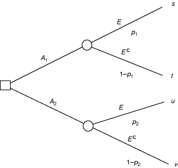
10.10 Decision Trees

This is a convenient place to introduce a pictorial device that is often very useful in thinking about a decision problem, using Table 10.3 as an example. The fundamental problem is a choice between A₁ and A₂. This choice is represented by a decision node, drawn as a square, followed by two branches, one for A₁ and one for A₂, as in Figure 10.1. If A₁ is selected, either E or E ^c arises, where the outcome, unlike a decision node, is not in your hands but rests on uncertainty and is therefore represented by a random node, drawn as a circle, followed by two branches, one for E, one for E ^c (Figure 10.1). Their respective probabilities may be used as labels for the branches. The case (§10.6) where these may depend on the act has been drawn. Similar nodes and branches follow from A₂. Finally, at the ends of the last 4 branches we may write the utilities of the 4 consequences, like fruit on the tree, and Figure 10.1 is complete. It is called a decision tree but, unlike nature's trees, it grows from left to right, rather than upright, the growth reflecting time, the earlier stages on the left, the final ones, the consequences, on the right. Clearly any number of branches, corresponding to acts, may proceed from a decision node, not just two as here, and any number, corresponding to events, from a random node. Although time flows from left to right, the analysis proceeds in reverse time order, from right to left, from the imagined, uncertain future back to now, the choice of act. To see how this works, consider the upper, random node, that flowing from A₁, where the branches following, to the right, can be condensed to provide the expected utility (cf. Equation (10.6)) on multiplying each utility on a branch by its corresponding probability and adding the results. Similarly at the random node from A₂ there is an expected utility and, going back to the decision node, the choice between A₁ and A₂ is made by selecting that with the larger expected utility. The general procedure is to move from right to left, taking expectations at a random node and maxima at a decision node.

It is easy to see how to include another event in the tree as in §10.9. Consider the upper branches in Figure 10.1 proceeding through A₁ and E. Another random node followed by two branches, corresponding to the extra events F and F ^c, may be included as in Figure 10.2 with utilities s₁ and s₂ at their ends, replacing the original utility s. Again we proceed from the far right, obtaining at the random node for F and F ^c, expected utility

that, we saw in §10.9, equals s, and we are back to Figure 10.1. Similar extensions may be made at the three other terminations of Figure 10.1. Notice again, the equivalence between the expected utility and the original utility.

The real power of a decision tree is seen when there is a series of decisions that have to be made in sequence, one after another, with uncertain events occurring between. Without going into detail and exhibiting the complete, large tree, consider a medical example where, as above, there is initially a choice between two treatments A₁ and A₂. Let us follow A₁ and suppose event E occurs, that the patient develops complications, when a further decision about treatment may need to be made. Suppose treatment B is selected and event F then occurs. The corresponding part of the tree is given in Figure 10.3. Probabilities may be placed on the branches proceeding from the random node. In principle the tree could continue forever with a contemplated series of acts and events but, in practice, it will be expedient to stop after a few branches. When it does, utility evaluations may be inserted at the right-hand ends. In the example, it is natural to stop after F. Analysis of the tree is simple in principle: proceed from right to left, at each random node calculate an expected utility, at each decision node select the branch with maximum expected utility. In the example of Figure 10.3, at the final, random node the probability on each branch, of which only one is shown, is multiplied by the terminal utility and the results added, giving the expected utility of B. With a similar procedure for the actions alternative to B, that act among them of maximum expected utility may be selected. This maximum effectively replaces the branches labeled B and F in Figure 10.3, and we are back to the simple form of Figure 10.1, except that we have only drawn the uppermost sequences of branches, and a choice made, as there, between A₁ and A₂.

Notice how the analysis of the tree proceeds in reverse time order, from the acts and events in the future back to the present decisions. This is reflected in an issue that applies generally in life and is captured succinctly in the epigram:

you cannot decide what to do today until you have decided what to do with the tomorrows that today's decisions might bring.

A beautiful example of this is to be found in §12.3 where a decision is taken that, in the short term is disadvantageous but, in the long term, yields an optimum result. The medical example of Figure 10.3 illustrated this, for a choice between A₁ and A₂ now depends on events like E and what act, like B, will be necessary to take tomorrow. The construction of a decision tree demands that you think not solely in terms of immediate effects but with serious consideration of longer term consequences. Of course the tree will have to stop somewhere but the timescale depends very much on the nature of the problem. The little problem of which coat to wear need scarcely go beyond that day, but decision problems about nuclear waste may need to consider millennia.

10.11 The Art and Science of Decision Analysis

The construction of a decision tree is an art form of real value, even when separated from the numeracy of the science of probabilities and utilities, and the analysis through maximization of expected utility. Thinking within the framework of the tree encourages, indeed almost forces, you to think seriously about what might happen and what the consequences could be if it did. Then again, like all good art, it is a fine communicator in that it clearly presents to another person the problem laid out in a form that is easily appreciated. Even if the reader is uncomfortable with numeracy, despite the persuasive arguments that have been used here, such a person can value the clarity of the tree. They might also be impressed by the power and convenience that trees offer. Decisions today affect decisions tomorrow. Events today affect events tomorrow. The numerical approach offers a principled way to combine these factors to make a sound recommendation for what to do now. I look forward to an enlightened age when it will be thought mandatory for any proposal for action to be accompanied by its decision tree.

Unfortunately, the happy situation of the last sentence will not easily come about because people in power perceive a gross disadvantage in trees and their associated probabilities and utilities; namely that trees expose their thinking to informed criticism. Partly this arises for the reason just given, that a decision tree is good art and therefore a good communicator exposing the decision maker's thinking to public gaze. But there is more to it than that, for the study of the tree reveals what possible actions have been considered and how one has been balanced against another. Also the tree tells us what uncertain events have been considered: did a firm take into account accidents to the work force, or only shareholders' profits? This is before numeracy enters and the uncertainties and consequences measured. Were they to be included, then the exposure of the decision maker's views would be complete. Although probabilities have made some progress toward acceptance so that, for example, one does see statements about the chance of dying from lung cancer, utilities are hardly ever mentioned, in my view because they expose the real motivations behind a recommendation for action. An example will be met in §14.6, where the current financial crisis is discussed. The bankers' decision-making may not have used MEU, but even if it did the bankers have been silent about their utilities.

The introduction of decision trees, while it would go some way to make society more open, would expose a more fundamental difficulty, the difference between personal and social utility, between the desires of the individual and those of society. This is a conflict that has always been with us and is clearly exposed by the apparatus of a decision tree. Here is an example. An individual automobile driver, unencumbered by speed limits, may feel that his utility is maximized by driving fast. Partly to protect others on the road and partly because such a driver may underestimate the danger to himself of driving fast, we have agreed democratically to speed limits, and to fines for speeders. We pay police to enforce these laws, and we pay fines if we speed and are caught. We do so in order to change the individual utilities of drivers, to make it individually optimal for them to drive more slowly.

The two utilities, of the individual and of society, are in conflict and my own view is that a major unresolved problem is how to balance the wishes of the individual against those of society. This is another aspect of the point mentioned in §5.11 that the contribution that the methods here described make toward our understanding of uncertainty and its use in decision analysis, do not apply to conflict situations. Our view is personalistic. This is not to say that the ideas cannot be applied to social problems, they can; but they do not demonstrate how radically different views may be accommodated. The way we proceed in a democratic society is for each party to publish its manifesto, or platform, and for the electorate to choose between them. An extension, in the spirit of this book, would be for the platforms to include probabilities but especially utilities. While this system may be the best we have, it has defects and there is a real need for a normative system that embraces dissent and is not as personalistic as that presented here, though recall that the “you” of our method could be a government, at least when it is dealing with issues within the country. It is principally in dealing with another government that serious inadequacies arise.

Our study of decision analysis does reveal one matter that is often ignored, especially in elections. However you structure decision making, either in the form of a table or through a tree, the choice is always between the members of a list of possible decisions from which you select what you think is the best. To put it differently, it makes no sense to include another row in your table, or another branch in your tree, corresponding to “do something else”. Nor, when the uncertain events are listed, does it make sense to include “something else happens.” In both cases it is essential to be more specific, for otherwise the subsequent development along the tree cannot be foreseen, nor the numeracy included. It is not sensible, as a politician suggested, to distinguish between known unknowns and unknown unknowns. Everything is a choice between what is available. We have mentioned that the construction of a decision tree is an art form and one of the main contributions to good art is the ability to think of new possibilities. Scientific method is almost silent on this matter, except to make one aware of the need for innovation, yet it is surely true that some good decision making has come about through the introduction of a possibility that had not previously been contemplated. However, once ingenuity has been exhausted, only choice remains:

One does not do something because it is good, but because it is better than anything else you can think of.

In particular, you should vote in an election and choose the party that you judge to be the best, for to deny yourself the choice allows others to select.

A related merit of decision trees is that they encourage you to think of further branches, either relating to an uncertain event or to another possible action. For example, it has been suggested that good decision makers are characterized by their ability to think of an act that others have not contemplated. It is even possible that the art of making the tree is more important than the science of solving it by MEU. Of course, one has to balance the complication that arises from including extra branches against the desire for simplicity.

10.12 Further Complications

Before we leave decision analysis, there is one matter, more technical in character, that must be mentioned. To appreciate this, return to Figure 10.3, which is part of a decision tree in which action A₁ resulted in an event E, to which the response was a further act B, followed by an event F, so that the time order proceeds from left to right. Here A₁ is the first, and F the last, feature. At the end of the tree, on the right, it is necessary to insert a utility in the form of a number. The point to make here is that this utility, describing the consequence of acts A₁ and B with events E and F, could depend on all four of these branches, though not, of course, on other branches like A₂, which do not end at the same place. Mathematically the utility of a consequence is a function of all branches that lead to that consequence; here . Thus it would typically happen that A₁, a medical treatment, would be costly in time, money, and equipment, resulting in a loss of utility in comparison with a simpler treatment like A₂. Exactly how this is incorporated into the final utility is a matter for further discussion; all that is being said here is that the cost should be incorporated. Similarly E may have costs, both in terms of hospital care and through long-term effects.

Similar remarks apply to the probabilities on the branches emanating from random nodes. They can depend on all branches that precede it to the left, before it in time. We have repeatedly emphasized that probability depends on two things: the uncertain event and the conditions under which the uncertainty is being considered. The latter includes both what you know to be true and what you are supposing to be true. This applies here and, for example, at the branch labeled with the uncertain event F, the relevant probability is since A₁, E, and B precede F and you are supposing them to be true. Similarly you have . It often happens that some form of independence obtains, for example that given E and B, F is independent of A₁. This can be expressed in words by saying that the outcome of the second act does not depend on the original act but only on its outcome. We may then write , omitting A₁. Such independence conditions play a key role in decision analysis, in particular, making the calculations much simpler than they otherwise would be.

Many people are unhappy with the wand device that was used to construct our form of utility, so let us look at it more carefully and use as an example a situation where you are trying to assess the utility of your present state of health. Here you are asked to contemplate a magic wand, which would restore you to perfect health but might go wrong and kill you. You are being asked to compare your present state with something better and with something worse, the comparison involving a probability u that the wand will do its magic, and 1 − u that it will cause disaster. With perfect health having utility 1, disaster utility 0, u is the least value you will accept before using the wand and is the utility of your present state. Many people object to the use of an imaginary device, or what is often called a thought experiment, namely an experiment that does not use materials but only thinking. Since you have of necessity to think about a consequence, the procedure may not be unreasonable. Recall too, the point made above, that we have to make choices between actions, so that anyone who objects to wands must produce an alternative procedure. Indeed, there are two questions to be addressed:

As has been said before, utility as probability answers the second question extremely well. As to the first, notice that the wand at least provides a sensible measure. If your current state of health is fairly good, the passage to perfect health would not be a great improvement, so only worth a small probability of death. The last phrase means 1 − u is small and therefore u is near one. On the contrary, if you are in severe pain, perfect health would be a great advance, worth risking death for, and 1 − u could be large, u near 0. So things go in the right direction, but there is more to it than that, for the probability connection enables us to exploit the powerful, basic device of coherence.

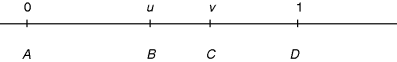
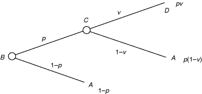
To see how this works consider four consequences labeled A, B, C, and D, the more advanced the letter in the alphabet, the better it is, so A is the worst, utility 0; D is the best, utility 1. B and C are the intermediates with utilities u and v, respectively, with u less than v. (See Figure 10.4). These values will have been obtained by the wand device using A and D as before. Now another possibility suggests itself; since B is an intermediate between A and C, why not consider replacing B by a wand that would yield C with probability p and A with probability 1 − p. How should p relate to u and v ? This is easily answered, for you have just agreed to replace B by a probability p of C, and previously you have agreed to replace C by a probability v of D. Putting these two statements together by the product rule, you must agree that B can be replaced by a probability pv of D. (In all these replacements, the alternative is A.) But earlier B had been equivalent to a probability u of D, so therefore

You may prefer to use a tree as in Figure 10.5 with random nodes only and the probabilities, necessarily adding to 1, at the tips of the tree. These considerations lead to the following practical device: Use three wands to evaluate u, v, and p; then check that indeed p = u /v. If it does, you are coherent; if not, then you must need to adjust at least one of u, v, and p so that it is true for the adjusted values and coherence is obtained. Without coherence, you would be a perpetual, money-making machine (see §10.2).

There is more, for consider replacing C by a wand with probability q of D and 1 − q of B. How is q related to u and v ? Since B can be replaced by a probability 1 − u at A, C must be equivalent to a probability of A by the product rule again. But you previously agreed that C could be replaced by 1 − v at A, so

and a further coherence check is possible. The important, general lesson that emerges from these considerations is that if you need to contemplate several consequences (at least four) then there are several wands that you can use, not just to produce a utility for each consequence but also to check on coherence. Indeed, as with probability, there is a very real advantage in increasing the numbers of events and consequences, because you thereby increase the opportunities for checks on coherence. The argument is essentially one for coherence in utility, as well as in probability, resulting in coherence in decision analysis.

10.13 Combination of Features

The ability to combine utility assessment with coherence becomes even more important when the consequences involved concern two, or more, disparate features. To illustrate, consider circumstances that have two features, your state of health and your monetary assets. To keep things simple, suppose there are two states of health, good and bad; and two levels of assets, high and low. These yield four consequences conveniently represented in Table 10.5.

Table 10.5 Consequences with two features.

		Assets
Health	Low	High
Good	u	1
Bad	0	v

The consequence of both good health and high assets is clearly the best; that of bad health with low assets the worst, so you can ascribe to them utilities 1 and 0, respectively and derive values u and v for the other two, as shown in the table. Notice this table differs from earlier ones in that no acts are involved. Suppose you are in bad health with high assets, utility v, and that u = v, then you would be equally content, because of the same utility, with good health and low assets. Expressed differently, you would be willing to pay the difference between high and low assets to be restored to good health. If v exceeds u, v > u, you would not be prepared to pay the difference; but if u exceeds v, u > v, you would be willing to pay even more.

In reality assets are on a continuous scale and not just confined to two values; similarly health has many gradations. It is then more convenient to describe the situation as in Figure 10.6 with two scales, that for assets horizontally, increasing from left to right; that for health vertically, the quality increasing as one ascends. In this representation you would want to aim top-right, toward the northeast, whereas unpleasant consequences occur in the southwest. Without any consideration of uncertainty or any wands, you could construct curves, three of which are shown in the figure, upon any one of which your utility is constant, just as u might equal v in the tabulation. Moving along any one of these curves, as from A to B in the figure, your perception of utility remains constant and the loss in assets results in an improvement in health. Movement in the contrary direction might correspond to deteriorations in health caused by working hard in order to gain increased assets. The same type of figure will be found useful when financial matters are studied in §14.6.

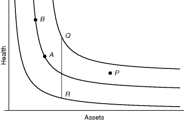
The further northeast the curves are, the higher your utility on them, and to compare the values on different curves you could use a thought experiment of the type already considered. For example, suppose you are at P with high assets but intermediate health, you might think of an imaginary medical treatment that could either improve your health to Q or make it worse at R, but costing you money, so, losing you assets. What probability of improvement would persuade you to undertake the treatment? There are many thought experiments of this type that would both provide a utility along a curve and also check on coherence. What this analysis finally achieves is a balance between health and money, effectively trading one for the other. Modern society uses money as the medium for the measurement of many things, whereas decision analysis uses the less materialistic and more personal concept of utility. People who have a lot of money often say “money isn't everything”, which is true, but utility is everything because, in principle, it can embrace the enjoyment of a Beethoven symphony or the ugliness of a rock concert, thereby revealing an aspect of my utility. One aspect that is too technical to discuss in any detail here is the utility of money or, more strictly, of assets. Typically you will have utility for assets like that shown in Figure 10.7, where you attach higher utility to increased assets, but the increase of utility with increase in assets flattens out to become almost constant at really high assets. For example, the pairs (A, B) and (P, Q) in the figure correspond to the same change of assets but the loss in utility in passing from A to B is greater than that from P to Q. For most of us, the loss of 100 dollars (from P to Q, or A to B) is more serious when we are poor at A, than when we are rich at P. A utility function like that of Figure 10.7 can help us understand lots of monetary behavior and is the basis, often in a disguised form, of portfolio analysis when one spreads one's assets about in many different ventures. Notice that we have used assets, not as often happens, gains or losses, in line with the remarks in §10.6. It is where you are that matters, not the changes. Another feature of Figure 10.7 is that utility is always bounded, by 1 in the figure. There are technical reasons why this should be so and the issue rarely arises in practice.

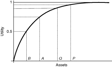
The discussion around Figure 10.6 revolved around two features, there health and money, but the method extends to any number of features, though a diagrammatic representation is not possible. The idea is to think of situations that, for you, have the same utility, forming curves in Figure 10.6, but imagined surfaces with more than two features, finally using thought experiments to attach numerical values to each surface. Here is an example which arose recently in Britain, where “you” is the National Health Service (NHS). Thus we are talking about social utility, rather than the utilities of individuals (see §10.11). The three features are money, namely the assets of the NHS, the degree of multiple sclerosis (MS), and the degree of damage to a hip. Notice that we do not need to measure these last two features, any more than we did health in the earlier example, utility will do that for us in the context of a decision problem. The decision problem that arose was inspired by the introduction of a new drug that was claimed to be beneficial to those with a modest degree of MS but was very expensive. There were doubts concerning how effective it was, but let us ignore this uncertainty while we concentrate on the utility aspects. The NHS decided the drug was too expensive to warrant NHS money being spent on it. This decision naturally angered sufferers from MS who pointed out that the expected improvement in their condition would enable them to work and thereby save the NHS on invalidity benefit. Where, you may ask, does the hip damage come in? It enters because the money spent on one patient with MS could be used to pay for 10 operations to replace a hip. So the NHS effectively had to balance 10 good hips against one person relieved of MS. Other features in lieu of hips might have been used, for the point is that in any organization like the NHS, there are only limited resources and, as a result, hips and MS have to be compared. Our proposal is that the comparison should be effected by utility, and the suggestion made that this utility be published openly for all to see and comment upon. One can understand the distress to sufferers from MS by the denial of the drug but equally the discomfort of 10 people with painful hips has to be thought about. People are very reluctant to admit that there is a need for a balancing act between MS and hips, but it is so. Utility concepts are a possible way out of the dilemma, though, as mentioned before, they do not resolve the conflict between personal and social utility.

10.14 Legal Applications

Consider the situation in a court room, where a defendant is charged with some infringement of the law, and suppose it is a trial by jury. There is one uncertain event of importance to the court—Is the defendant guilty of the offence as charged?—which event is denoted by G. Then it is a basic tenet of this book that you, as a member of the jury, have a probability of guilt, , in the light of your background knowledge . (There are many trials held without a jury, in which case “you” will be someone else, like a magistrate, but we will continue to speak of “juror” for linguistic convenience.) We saw in §6.6 how evidence E before the court would change your probability to using Bayes rule. The calculation required by the rule needs your likelihood ratio , involving your probabilities of the evidence, both under the supposition of guilt and of innocence, G ^c. It was emphasized how important it was to consider and to compare evidence in the light both of guilt and of innocence.

Before evidence is presented, it is necessary to consider carefully what your background knowledge is. As a member of the jury, you are supposed to be a representative of society and to come to court with the knowledge that a typical member of society might possess. As soon as the trial begins, you will learn things, like the formal charge; and you will also see the defendant, so enlarging . At this point you may be able to contemplate a numerical value for your probability. For example, if the charge is murder, where all admit that a person was killed, you may feel it reasonable to let , where N is the population of the country to which the law pertains, on the principle that someone did the killing and until specific evidence is produced, no person is more probable than any other. (The law says all are innocent until proved guilty but that is not satisfactory since it says in default of Cromwell's rule, for someone did the killing.) If evidence comes that the killing was particularly violent and must have been committed by a man, you may wish to replace N by the number of adult males.

There are cases where the assignment of the initial probabilities, , is really difficult. Suppose the charge is one of dangerous driving in which all accept that a road accident occurred with the defendant driving. Also suppose the only point at issue is whether the defendant's behavior was dangerous or whether some circumstance arose which he could not reasonably have foreseen. One suggestion is to say that initially you have no knowledge and both possibilities are equally likely, so ½. But this is hardly convincing since several different circumstances might equate to the defendant's innocence, so why not put if you can think of n different circumstances?

A possible way out of difficulties like these is to recognize that your task as a juror is to assess the defendant's guilt in the light of all the evidence, so that fundamentally all that you need is , where E is the totality of the evidence. The point of doing calculations on the way as pieces of evidence arrive is to exploit coherence and thereby achieve a more reasonable final probability than otherwise. As a result of these ideas, one possibility is to leave until has been inflated by some of the evidence, sufficient to give you some confidence in your probability, and only then exploit coherence by updating with new evidence. There is no obligation to assess every probability; we have a framework which can be as big or as small as you please, increased size having the advantage of more coherence. The situation is analogous to geometry. You might judge that a carpet will fit into a room, or you may measure both the carpet and the room and settle the issue. The measurement uses geometrical coherence, direct judgment does not but may be adequate. The ideas here are related to the concepts of small and large worlds (§11.7).

In using the coherence argument in court, a difficulty can arise when two pieces of evidence are presented. Omitting explicit reference to the background knowledge in the notation, because it stays fixed throughout this discussion, the first piece of evidence, E₁, will change your probability to . When the second piece of evidence E₂ is presented, a further use of Bayes rule will update it to and the relevant likelihood ratio will involve and . (To see this apply Bayes rule with all probabilities conditional on at least E₁.) To appreciate what is happening, take the case where the two pieces of evidence are of different types. For example, E₁ may refer to an alibi and E₂ to forensic evidence provided by a blood stain. If you judge them to be independent (§4.3) given guilt and also given innocence, so that , the updating by E₂ is much simpler since E₁ is irrelevant. In contrast, take the position where they are both alibi evidence, then you may feel that the two witnesses have collaborated and the independence condition fails. In which case you might find it easier to consider E₁E₂ as a single piece of evidence and update p (G) to directly without going through the intermediate stage with only one piece of evidence. Independence is a potentially powerful tool in the court room but it has to be introduced with care.

At the end of the trial the jury is asked to pronounce the defendant “guilty” or “not guilty”; in other words, to decide whether the charge is true or false. According to the ideas presented in this book, the pronouncement is wrong, for the guilt is uncertain and therefore what should be required of the jury is a final probability of guilt. Hopefully this might be near 0 or 1, so removing most of the uncertainty, but society would be better served by an honest reflection of indecision, such as probability 0.8. Actually the current requirement for “guilt” is “beyond reasonable doubt” in some cases and “on the balance of probabilities” in others. For us, the latter is clear, probability in excess of one half, but the former, like most literary expressions, is imprecise and senior judges have been asked to say what sort of probability is needed to be beyond reasonable doubt; essentially what is “reasonable”? The value offered may seem low, a probability of 0.8 frequently being proposed. A statistician might say at least 0.95. I think the question of guilt is wrongly put and that the jury should state their probability of guilt.

There is an interesting separation of tasks in an English court, where the jury pronounces on guilt but the judge acts in passing sentence, which is automatic in the case of a “not guilty” verdict. This is somewhat in line with the treatment in this book, the jury dealing with probability, the judge dealing in decision making. If judges are to act coherently they will need utilities to combine with the probability provided by the jury. The broad outlines of these utilities could be provided by statute, though the judge would surely need some freedom in interpretation since no drafting can cover all eventualities. As an example, I suggest that instead of saying that a maximum fine for an offence should be 100 dollars, perhaps 1% of assets might be a more reasonable maximum, so that a rich person's illegal parking could have a significant effect on reducing taxes. The point here is that a fine is not a way of raising money but a deterrent, so that 100 dollars deters the poor more than the rich. Utility considerations could also reflect findings in penology.

The thesis of this book impinges on court practice in other ways. The law at the moment rules that some types of evidence are inadmissible, so that they are denied to the jury, though the judge may be aware of them in passing sentence. However, it was seen in §6.12 that data, or evidence, is always expected to be of value, in the sense that your expected value of the information provided by evidence is always positive; so that, as a member of the jury, you would expect the inadmissible evidence to help you in your task. Evidence has a cost that needs to be balanced against the information gain, using utility considerations as in §10.13. Hence the recommendation that flows from our thesis is that the only grounds for excluding evidence are on grounds of cost. It has been argued by lawyers that evidence should be excluded because jurors could not handle it sensibly. This is a valid argument in the descriptive mode but ceases to be true in the normative position. When the jurors are coherent, all evidence might be admitted.

Another way in which probability could affect legal practice is in respect of the double jeopardy rule whereby someone may not be tried twice for the same offence. If new evidence arises after the completion of the original trial and is expected to provide a lot of information, then the court's probability will be expected to be changed. The present rule may partly arise through the jury's being forced to make a definite choice between “guilty” and “not guilty” and the law's natural reluctance to admit a mistake. With an open recognition of the uncertainty of guilt by the jury stating a probability, what had been perceived as a mistake becomes merely an adjustment of uncertainty. The case for every juror, and therefore every citizen, having an understanding of uncertainty and coherence becomes compelling.

There is one aspect of the trial that our ideas do not encompass and that is how the individual jurors reach agreement; how do the twelve “yous” become a single “you”? This was mentioned in §10.8. A rash conjecture is that if coherence were exploited then disagreement might be lessened. Another feature of a trial that needs examination in the light of our reasoned analysis is the adversarial system with prosecution and defense lawyers; a system that has spread from the law to politics in its widest sense where we have pressure groups whose statements cannot be believed because they are presenting only one side of the case. After all, there is another method of reaching truth that has arguably been more successful than the dramatic style that the adversarial system encourages. It is called science and is the topic of Chapter 11.

The above discussion only provides an outline of how our study of uncertainty could be used in legal contexts, namely as a tool that should improve the way we think about the uncertain reality that is about us. While it is no panacea, it is a framework for thinking that has the great merit of using that wonderful ability we have to reason, which yet enables our emotional and other preferences to be incorporated. The calculus of probability has claim to be one of the greatest of human kind's discoveries.