
Chapter 16
Aid Allocation: A Complex Perspective
Robert J. Downes and Steven R. Bishop
16.1 Aid Allocation Networks
16.1.1 Introduction
While much has been written on foreign aid allocation, relatively little work has considered mathematical models beyond regression analysis. Modelling aid allocation is a complex issue. Empirical findings on the allocation of foreign aid indicate that donor countries pursue a wide range of objectives, achieving complex outcomes sometimes with unintended consequences. Poverty alleviation is frequently cited as a key factor in the disbursement of aid, see United Kingdom Government 2002, United States Government 1961, Collier and Dollar 2002; donor countries often engage in less than altruistic behaviour, see Harrigan and Wang 2011; highly heterogeneous behaviour is the norm, see Collier and Dollar 2002, Harrigan and Wang 2011, Alesina and Dollar 2000, Bermeo 2008, Berthélemy 2006, and Balla and Reinhardt (2008). Recent research indicates that decision-making in the donor community also impacts the allocation of aid (see Riddell 2007 and Frot and Santiso 2011). Such ‘bandwagon’ behaviour is widely recognised in financial markets, see Schiller 2000 and Hommes 2006, but has only recently been considered as a component of aid allocation.
The development of mathematical models can support thinking on aid allocation and effectiveness. Most mathematical models follow a statistical trajectory, postulating a range of variables upon which aid allocation depends, followed by a regression-based analysis of available data; McGillivray 2003, Berthélemy 2006, Alesina and Dollar 2000 and Tarp et al. 1999 give an excellent introduction to this approach. Other models take an econometric route, considering a utility maximisation process, often based on recipient need; Collier and Dollar 2002, Chong and Gradstein 2008 and Tarp et al. 1999 all cover such procedures and McGillivray 2004 gives a particularly delicate consideration in the context of so-called ‘prescriptive and descriptive’ analyses of aid allocation.
This chapter presents a novel formulation of aid allocation. Rather than adopting a statistical or data-driven approach, we develop a framework allowing the model user to explore the allocation of foreign aid through the mathematical theory of networks. We aim to allow users of this model to explore possible policy choices in aid allocation. Statistical analysis indicates how donor countries have allocated aid in the past. Looking forward, our model allows users to explore responses to this analysis. Highlighting the behaviour of donor countries, we focus on the complexity of aid allocation from a mathematical perspective. According to McBurney 2012, alternative perspectives can function as a ‘locus of discussion’ which
provide[s] a means to tame the complexity of the domain. Modelling thus enables stakeholders to jointly explore relevant concepts, data, system dynamics, policy options, and the assessment of potential consequences of policy options, in a structured and shared way.
This is our intention throughout this chapter.
16.1.2 Why Networks?
The community of aid donors and recipients is complex in a mathematical sense. According to Wilson 2012:
Complex systems are characterised by requiring many variables to describe them and having strong interdependencies between the elements of the system. When represented mathematically, these interdependencies will typically be nonlinear relationships.
In the aid allocation context, complex systems exhibit emergent behaviour: decisions made by individual system actors aggregate into global system states in an often unpredictable manner. Whether global states are desirable or otherwise is beyond the purview of any individual actor.
A motivating example from population studies is given in Schelling 1971: the population comprises two groups randomly distributed on a lattice (finite in extent); individuals have a preference for remaining close to members of their own group and will move accordingly in a series of discrete steps. The model demonstrates that each actor's relatively small preference for being close to members of its own group can lead to a global pattern of segregation and that, famously, ‘inferences about individual motives can usually not be drawn from aggregate patterns’.
As currently available models of aid allocation are typically statistically oriented, only qualitative discussion of complex behaviour is possible, see for example Ramalingam (2011). Mathematical models allowing users to explore the complexity of aid allocation are therefore a valuable contribution to current discussion.
16.1.3 Donor Motivation in Aid Allocation
Overviews of donor behaviour in aid allocation are provided by the work of Alesina and Dollar 2000 and Fuchs et al. 2014: donor countries do not behave uniformly towards recipient countries [Berthélemy 2006 and Chong and Gradstein 2008], and aid allocation generally depends upon the specific situation in recipient and donor nations (both in demographic and political terms).
A selection of common donor motivations includes poverty alleviation Collier and Dollar (2002), McGillivray 2003, Baulch 2003; colonial ties Alesina and Dollar (2000); commercial interests Harrigan and Wang (2011), Alesina and Dollar (2000), Younas (2008); strategic interests Harrigan and Wang (2011); governance and policy environment quality Collier and Dollar (2002), Burnside and Dollar (2004), McGillivray (2006). Recent work suggests that donor community bandwagon effects Frot and Santiso (2011), conflict Balla and Reinhardt (2008) and [im]migration Bermeo (2008) also play a role. Contenting ourselves with these factors throughout this chapter, we emphasise that this is not an exhaustive list.
The factors motivating donors can be divided into two distinct classes:
- 1. Factors associated with individual countries. These include governance quality and demographic factors related to poverty;
- 2. Factors associated with relationships between countries. These include colonial ties and commercial interests in the form of trade flows.
This division is essential in this chapter as we relate donor behaviour to an underlying network of countries.
There are many ways to classify social phenomena in complex systems. For example, in the context of ethno-political conflict, Gallo 2013 classifies contributory factors as so-called ‘state’ or ‘activity’ variables: state variables define structural aspects of the system, while activity variables are used to affect change in this structure.
16.2 Quantifying Aid via a Mathematical Model
16.2.1 Overview of Approach
In this section, we write down the basic mathematical objects used in this chapter. We do not assume the reader to be familiar with network theory and so include illustrative diagrams wherever possible. The mathematical details are kept to a bare minimum. We direct the interested reader to Newman 2010 for an accessible introduction to the theory of networks.
We base our model on an underlying network comprising a set of nodes connected by a number of different quantifiable relationships: nodes are identified with countries, and links between nodes with international relationships, material or otherwise. By further identifying countries as either donors or recipients and associating demographic information to each country, we construct a model of the international network of nations.
To each donor–recipient pair, we assign a function determining the preference the donor has for awarding aid to the recipient. This function is dependent upon the following:
- 1. Demographic information of donor and recipient;
- 2. Relationships between donor and recipient;
- 3. Relationships between donor and all other recipients (explicitly).
- 4. Relationships between donor and all other donors via all recipients (implicitly).
Allocations are made on the basis of this preference along with a minimum donation value below which donations are zero.
Demographic and relational information encoded in the network is related to donor behaviours discussed in Section 16.1.3: the model then simulates donor behaviour and subsequent aid allocation. For example, we explore the complex interaction between donors allocating aid for poverty alleviation and commercial gain simultaneously.
The preference function is stimulated by the generalised Cobb–Douglas production function see Cobb and Douglas 1928. In its original guise, this provides a functional relationship between two inputs, capital and labour, with production as output; the parameters governing this interaction are estimated statistically in Cobb and Douglas 1928. While the specification of the function is arbitrary, see Simon and Levy 1963, its utility can be seen in its simple presentation, understandability and elucidation of the complex interaction between factors and output of production, see (Bhanumurthy, 2002).
The preference function also shares the form of the utility function found in weighted product method approaches to multi-objective optimisation (see Marler and Arora 2004). However, we do not adopt an optimisation approach here.
16.2.2 Basic Set-Up
A graph or, equivalently, network ![]() is a collection of nodes (or vertices), denoted
is a collection of nodes (or vertices), denoted ![]() , linked by ties (or edges), denoted
, linked by ties (or edges), denoted ![]() . In a bipartite graph, the node set is decomposed into two disjoint subsets: there are edges between nodes in each disjoint set, but no edges connecting nodes within the same set. In a complete bipartite graph, each node is connected to every node of the opposing disjoint set; this is illustrated in Figure 16.1(a).
. In a bipartite graph, the node set is decomposed into two disjoint subsets: there are edges between nodes in each disjoint set, but no edges connecting nodes within the same set. In a complete bipartite graph, each node is connected to every node of the opposing disjoint set; this is illustrated in Figure 16.1(a).
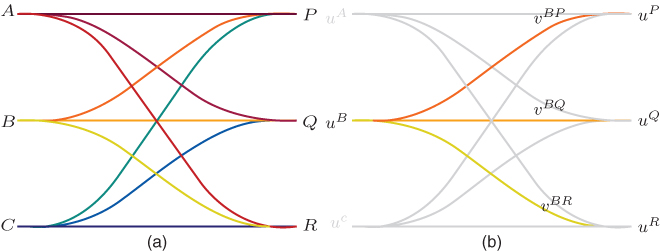
Figure 16.1 Complete bipartite graph (a) with vector weights and node-specific information detail (b)
A weighted graph has a numerical quantity associated with each edge. We work with a more general object, an ![]() -vector-weighted graph, in which
-vector-weighted graph, in which ![]() numbers are associated with each edge. Finally, we associate to each node an additional
numbers are associated with each edge. Finally, we associate to each node an additional ![]() numerical quantities which we call the
numerical quantities which we call the ![]() -vector node-specific information.
-vector node-specific information.
16.2.3 The Network of Nations
Define the network of nations as a complete bipartite ![]() -vector-weighted graph with
-vector-weighted graph with ![]() -vector node-specific information, with the following interpretation:
-vector node-specific information, with the following interpretation:
- Nodes represent countries,
 donor nations and
  recipient nations. We index donors and recipients by
  and
and  , respectively.
 - The vertex set
 is partitioned into donor and recipient country sets
  and
and  . No donors are recipients, or vice versa, and the total number of countries is
  .
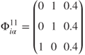
. - The
 -vector edge weights
  represent
  relationships between donor and recipient countries, material or otherwise. This will always be written so that the first superscript,
  , is donor
  and the second superscript,
  , is recipient
  . Then,
  is the
  element of the vector
  .
. - The
 -vector node-specific information
  represents
  quantities associated with each country
  in our network. Then
  is the
  element of vector
  . Donors and recipients will generally have different node-specific information, denoted by
  and
and  , respectively.
Figure 16.1(a) shows a network of nations with three recipients ![]() and three donors
and three donors ![]() ; appropriate
; appropriate ![]() -vector edge weights and
-vector edge weights and ![]() -vector node-specific information are given in Figure 16.1 (b).
-vector node-specific information are given in Figure 16.1 (b).
16.2.4 Preference Functions
In this model, aid is allocated using a preference function representing the preference a donor has for awarding aid to a recipient. For a given donor ![]() and recipient
and recipient ![]() , this function depends explicitly on
, this function depends explicitly on ![]() ,
, ![]() ,
, ![]() and
and ![]() ,
, ![]() where superscript • indicates ‘all countries in
where superscript • indicates ‘all countries in ![]() ’.
’.
For each donor ![]() and recipient
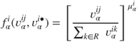
and recipient ![]() , define the preference function as
, define the preference function as
The functions ![]() ,
, ![]() and
and ![]() ,
, ![]() are to be specified for each donor
are to be specified for each donor ![]() .
.
Note that the functions ![]() and
and ![]() are country specific: in general, two different donors,
are country specific: in general, two different donors, ![]() and
and ![]() , have two different sets of functions
, have two different sets of functions ![]() and
and ![]() . Although we could suppress this additional generality, enforcing the same set of functions for all donors, we exploit this at a later stage when exploring donor heterogeneity.
. Although we could suppress this additional generality, enforcing the same set of functions for all donors, we exploit this at a later stage when exploring donor heterogeneity.
For clarity, consider the relationship defined by Equation (16.1): given donor ![]() and recipient
and recipient ![]() , for each component of
, for each component of ![]() , we have a function
, we have a function ![]() of
of ![]() and
and ![]() . Then
. Then ![]() depends on both the relationship between donor
depends on both the relationship between donor ![]() and recipient
and recipient ![]() and the relationship between donor
and the relationship between donor ![]() and all other recipients in
and all other recipients in ![]() . The same holds for functions
. The same holds for functions ![]() .
.
This construction therefore emphasises the role of the network of nations: the preference function assigned to each donor–recipient dyad depends upon both the dyad and all other recipients.
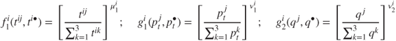
16.2.5 Specifying the Preference Functions
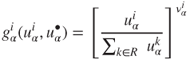
In applying the model, we must specify numerical quantities associated with the behaviour under investigation and, crucially, functions ![]() and
and ![]() for each donor
for each donor ![]() . While there is an arbitrariness in this specification, it can nonetheless provide insight into aid allocation.
. While there is an arbitrariness in this specification, it can nonetheless provide insight into aid allocation.
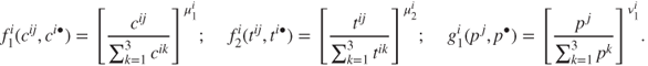
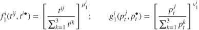
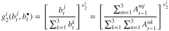
Here, the functions take the following form:
The role of the superscript • is seen in the denominator of the bracketed quantities in (16.2) and (16.3).
Equations (16.2) and (16.3) warrant the following explanation:
- Input (positive correlation): in (16.2) and (16.3), indicators positively correlated with aid allocation have the functional input
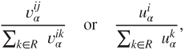
that is, as a proportion of the total
 between
  and all recipients, or the total quantity of
  among all recipients, respectively. A country with a greater proportion of a given quantity receives a greater allocation of preference and, hence, aid than a country with a lesser proportion.
 - Input (negative correlation): in (16.2) and (16.3), indicators negatively correlated with aid allocation have the functional input
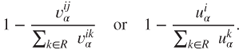
A country with a lesser proportion of a given quantity receives a greater allocation of preference and, hence, aid than a country with a greater proportion. In this case, we alter (16.2) and (16.3) accordingly.
- Parameters: the parameters
 and
and  can take values in
  , the positive real numbers including zero. All other things being equal, if a parameter takes
- the value 0: allocation is uniform;
- the value 1: allocation is strictly proportional;
- values in
 : allocation is ‘sub-proportional’, tending towards ambivalence as the parameter approaches 0;
 - values in
 : allocation is ‘super-proportional’, increasingly favouring the most preferred recipient as the parameter tends to
  .
.
16.2.6 Recipient Selection by Donors
In recipient selection, we assume there exists a minimum aid volume (a lower bound), ![]() , below which donor
, below which donor ![]() does not allocate. This threshold could be set uniformly for all donor nations and can also be set to zero.
does not allocate. This threshold could be set uniformly for all donor nations and can also be set to zero.
Each donor ranks all recipients by preference, then allocates aid to the largest subset of this ranking such that
- each recipient receives aid greater than or equal to the threshold
 ;
; - each recipient receiving aid has greater preference than all recipients not receiving aid.
If the threshold is set to zero, all donors receive some aid.
16.3 Application of the Model
16.3.1 Introduction
We illustrate the aid allocation model through three scenarios using the preference function (16.1), (16.2), (16.3) and the aforementioned model algorithm. All scenarios have the same set-up: three donors ![]() and three recipients
and three recipients ![]() . This situation is described by Figure 16.1. By varying donor behaviour, these scenarios emphasise different aspects of the model, especially system feedbacks.
. This situation is described by Figure 16.1. By varying donor behaviour, these scenarios emphasise different aspects of the model, especially system feedbacks.
Figure 16.2 gives a schematic representation of our model (with only a single donor ![]() present for clarity). Recipient states, donor states, donor–recipient relationships and donor community activity feed into
present for clarity). Recipient states, donor states, donor–recipient relationships and donor community activity feed into ![]() 's preference, determining aid allocation. In turn, this allocation affects the recipient states and the donor community in two feedback loops. This feedback is a simple source of complexity in the model and will be explored explicitly in the sequel.
's preference, determining aid allocation. In turn, this allocation affects the recipient states and the donor community in two feedback loops. This feedback is a simple source of complexity in the model and will be explored explicitly in the sequel.
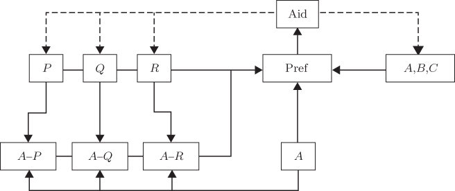
Figure 16.2 A schematic model representation with recipients  and donor
  . Arrows show information flows; dashed lines, feedback; hyphens, inter-country relationships
16.3.2 Scenario 1. No Feedback
This scenario examines the impact of heterogeneous donor motivation in aid allocation, introducing the model and its mode of operation. Donor motivation consists of recipient poverty ![]() , colonial relationships
, colonial relationships ![]() and trade flows
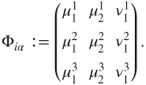
and trade flows ![]() (see Appendix A.1 for functional definitions). The scenario set-up is described in Figure 16.3; a detailed explanation of this figure is provided in Section 16.2.3. Note that all donors provide the same aid volume (normalised to 1); there is no minimum allocation threshold (see Section 16.2.6 for details).
(see Appendix A.1 for functional definitions). The scenario set-up is described in Figure 16.3; a detailed explanation of this figure is provided in Section 16.2.3. Note that all donors provide the same aid volume (normalised to 1); there is no minimum allocation threshold (see Section 16.2.6 for details).
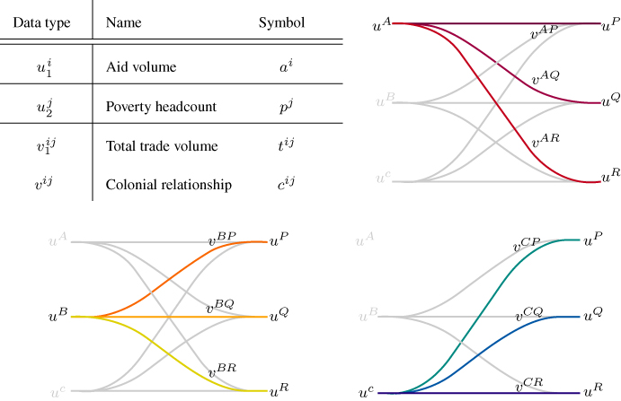
Figure 16.3 Scenario 1 set-up emphasising the role of node-specific information and inter-country relationships. The table notes the data included in this scenario, while each network diagram encodes relevant allocation data
The ratio of poverty headcount between recipient countries is ![]() ; trade relationships are the same for each donor, with the ratio between recipients given by
; trade relationships are the same for each donor, with the ratio between recipients given by ![]() , for
, for ![]() . Finally, for completeness,
. Finally, for completeness, ![]() is a former colony of
is a former colony of ![]() and
and ![]() while
while ![]() is a former colony of
is a former colony of ![]() .
.
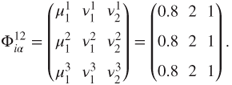
Using (16.1), (16.2) and (16.3), we write the preference function:
where
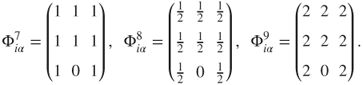
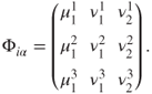
For ease, we take the matrix of parameters as
The choice of parameters governs the distribution of aid. We consider three different donor behaviours, showing the impact of (sub-/super-)proportional allocation (see Section 16.2.5).
Suppose alleviation of poverty is the only donor motive, and all donors value poverty identically (i.e. they have the same parameter choice). Let donors allocate proportionally, ![]() , sub-proportionally,
, sub-proportionally, ![]() and super-proportionally,
and super-proportionally, ![]() :
:
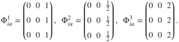
For each parameter choice, the allocation is given by Figure 16.4.
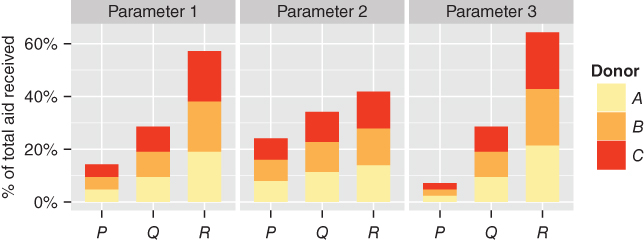
Figure 16.4 Model allocation for parameter choices 1, 2 and 3
The outcomes reflect recipient poverty headcount distribution, biased by donor motivation: when allocation is strictly proportional, ![]() , recipient
, recipient ![]() has 14% of total poverty and therefore receives 14% of total aid. Parameter choices
has 14% of total poverty and therefore receives 14% of total aid. Parameter choices ![]() and
and ![]() place, respectively, lesser and greater emphasis on poverty as a motivator of allocation, relative to the proportional allocation
place, respectively, lesser and greater emphasis on poverty as a motivator of allocation, relative to the proportional allocation ![]() .
.
Suppose that countries now allocate based on the poverty and colonial relationships. Again, let donors allocate proportionally, ![]() , sub-proportionally,
, sub-proportionally, ![]() and super-proportionally,
and super-proportionally, ![]() :
:
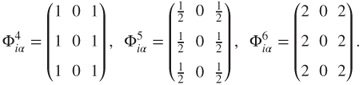
For each parameter choice, the allocation is given by Figure 16.5.
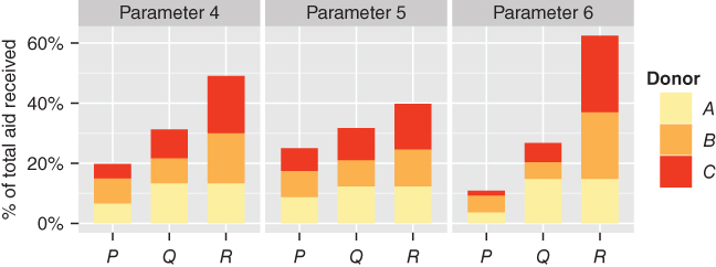
Figure 16.5 Model allocation for parameter choices 4, 5 and 6
In the proportional case (![]() ), including the positive aid allocation–colonial relationship, correlation in the preference function reduces by around 15% the allocation to
), including the positive aid allocation–colonial relationship, correlation in the preference function reduces by around 15% the allocation to ![]() , the recipient allocated most aid when poverty alone comprises donor behaviour, compared with the proportional allocation from Figure 16.4. In turn, the allocation to both
, the recipient allocated most aid when poverty alone comprises donor behaviour, compared with the proportional allocation from Figure 16.4. In turn, the allocation to both ![]() and
and ![]() increases, especially to
increases, especially to ![]() which is rewarded for its two colonial relationships with the donor community.
which is rewarded for its two colonial relationships with the donor community.
As earlier, parameter choices ![]() and
and ![]() place, respectively, lesser and greater emphasis on the overall combination of poverty and colonial history in aid allocation. Note also that
place, respectively, lesser and greater emphasis on the overall combination of poverty and colonial history in aid allocation. Note also that ![]() 's parameter choice is the same as that from Figure 16.4 as it has no colonies.
's parameter choice is the same as that from Figure 16.4 as it has no colonies.
These allocations are not obvious despite the simplicity of the situation (even assuming proportional allocation). In effect, identical signals from each recipient produce differing donor responses as a result of the unique set of donor–recipient relationships, even when donors share the same ‘values’ (parameter choices). This hints at the complexity of donor heterogeneity coupled with aggregation of aid flows.
Suppose now that commercial ties influence allocation, in addition to colonial relationships and poverty: donors reward recipients with whom they enjoy a large trade volume. Suppose that only ![]() and
and ![]() are influenced in this manner, with
are influenced in this manner, with ![]() steadfastly continuing to allocate based on poverty alone. Again, let donors allocate proportionally,
steadfastly continuing to allocate based on poverty alone. Again, let donors allocate proportionally, ![]() , sub-proportionally,
, sub-proportionally, ![]() and super-proportionally,
and super-proportionally, ![]() :
:
For each parameter choice, the allocation is given by Figure 16.6.
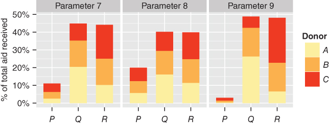
Figure 16.6 Model allocation for parameter choices 7, 8 and 9
While ![]() has the largest trade volume and poverty in absolute terms, overall donor behaviour has drawn aid away from the ‘most deserving’ recipient: aid is shared so that
has the largest trade volume and poverty in absolute terms, overall donor behaviour has drawn aid away from the ‘most deserving’ recipient: aid is shared so that ![]() , with middling poverty, strong colonial and modest trade relationships, is allocated approximately the same amount as
, with middling poverty, strong colonial and modest trade relationships, is allocated approximately the same amount as ![]() . This is in line with Alesina and Dollar 2000 who assert that former colonies are favoured over other nations; donors
. This is in line with Alesina and Dollar 2000 who assert that former colonies are favoured over other nations; donors ![]() and
and ![]() act in this way, while
act in this way, while ![]() is ‘Nordic’ in that it allocates based only upon need (see Alesina and Dollar 2000). This allocation with multiple criteria and heterogeneous donor motivation produces a radically different allocation to that given in Figure 16.4.
is ‘Nordic’ in that it allocates based only upon need (see Alesina and Dollar 2000). This allocation with multiple criteria and heterogeneous donor motivation produces a radically different allocation to that given in Figure 16.4.
This scenario highlights both the operation of the model and the complex interactions at the heart of aid allocation, emphasising that aggregate flows are a poor indicator of donor behaviour when heterogeneous multi-objective behaviour is the norm in the donor community.
16.3.3 Scenario 2. Bandwagon Feedback
Bandwagon behaviour is the tendency of donors to act in a self-reinforcing collective manner. Certain recipient countries gain ‘star’ status relative to others despite seemingly little difference between such nations. While this may be attributed to increasing selectivity of aid, the tendency of donors to reward effective aid usage - see Dollar and Levin (2006), recent work suggests that herd behaviour can play a significant role, see Frot and Santiso (2011). Recipients previously awarded large aid volumes are then preferred by the donor community and are rewarded as such in subsequent allocation. (Although selectivity is not considered here, it could be incorporated as a positively correlated effectiveness input with a super-proportional parameter choice.)
Donors allocate based on recipient poverty ![]() , commercial ties
, commercial ties ![]() and previous success in receiving aid
and previous success in receiving aid ![]() (see Appendix A.1 for functional definitions). The model is dynamic: with fixed demographic factors, aid volume changes as the model is iterated forward in time from
(see Appendix A.1 for functional definitions). The model is dynamic: with fixed demographic factors, aid volume changes as the model is iterated forward in time from ![]() . Donors reward recipients which are successful in garnering aid; this ‘community action’ affects subsequent allocation and corresponds to the clockwise feedback loop in Figure 16.2.
. Donors reward recipients which are successful in garnering aid; this ‘community action’ affects subsequent allocation and corresponds to the clockwise feedback loop in Figure 16.2.
The basic set-up of this scenario is as follows. Donors ![]() and
and ![]() allocate one unit of aid (
allocate one unit of aid (![]() ) while donor
) while donor ![]() allocates two units (
allocates two units (![]() ). As earlier, the ratio of poverty headcount between recipient countries is
). As earlier, the ratio of poverty headcount between recipient countries is ![]() . Only donor
. Only donor ![]() has significant trade relationships: the ratio between recipients is given by
has significant trade relationships: the ratio between recipients is given by ![]() .
.
Using (16.1), (16.2), and (16.3) we write:
where
We take the matrix of parameters as
We consider two different parameter choices, showing the impact of bandwagon feedback on the allocation of aid, driven by poverty and commercial interest, respectively.
Let all donors allocate according to recipient poverty and experience a sub-proportional tendency towards bandwagon behaviour (as this is a relatively subtle effect, see Frot and Santiso (2011)). Allocation based on poverty and bandwagon behaviour manifests in the following parameter choice:
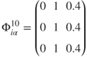
For this parameter choice, the aid allocation from ![]() to
to ![]() is given by Figure 16.7.
is given by Figure 16.7.
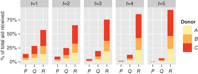
Figure 16.7 Model allocation for parameter choice 10
As we move forwards in time, it is clear that ![]() , the country allocated most aid based upon the poverty measure at
, the country allocated most aid based upon the poverty measure at ![]() , has increased its share of aid by approximately 50% at
, has increased its share of aid by approximately 50% at ![]() . Correspondingly, the country allocated least aid at
. Correspondingly, the country allocated least aid at ![]() ,
, ![]() , has seen its share of aid fall by a significant factor by
, has seen its share of aid fall by a significant factor by ![]() .
.
This illustrates the bandwagon phenomenon driven by aid volume: ![]() experiences an increase in aid allocation as a result of prior success in garnering aid. While a contrived example, this scenario demonstrates one approach to modelling bandwagon behaviour in the donor community.
experiences an increase in aid allocation as a result of prior success in garnering aid. While a contrived example, this scenario demonstrates one approach to modelling bandwagon behaviour in the donor community.
Suppose now that ![]() and
and ![]() allocate based on poverty, but
allocate based on poverty, but ![]() allocates based on commercial interests; all donors are subject to a sub-proportional bandwagon influence.
allocates based on commercial interests; all donors are subject to a sub-proportional bandwagon influence.
Allocation based on this situation manifests in the following parameter choice:
For this parameter choice, the aid allocation from ![]() to
to ![]() is given by Figure 16.8.
is given by Figure 16.8.
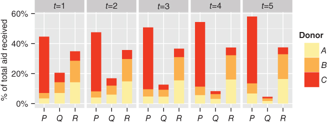
Figure 16.8 Model allocation for parameter choice 11
In this case, we see that the conflicting motivations of donor nations have produced a complex result. ![]() and
and ![]() prioritise
prioritise ![]() as the ‘neediest’ nation, but have also been drawn towards
as the ‘neediest’ nation, but have also been drawn towards ![]() via a bandwagon effect resulting from
via a bandwagon effect resulting from ![]() 's commercially driven aid allocation. As neither
's commercially driven aid allocation. As neither ![]() ,
, ![]() or
or ![]() prioritise
prioritise ![]() , the share of aid received by
, the share of aid received by ![]() and
and ![]() increases. If the strength of the bandwagon behaviour were stronger, the self-reinforcing behaviour would draw increasing volumes of aid from
increases. If the strength of the bandwagon behaviour were stronger, the self-reinforcing behaviour would draw increasing volumes of aid from ![]() toward
toward ![]() over time.
over time.
These two examples show the bandwagon allocation mechanism, albeit in an exaggerated manner. The first shows that, in our model, poverty itself can act as a driver of bandwagon behaviour: even though all nations prioritise poverty alleviation, they can be affected by the relative success of certain nations over time. The good intentions of donor nations can be subverted by their tendency towards ‘groupthink’.
The second example shows how, in our model, varying motives and donated aid volumes can lead to a complex allocation outcome in the presence of bandwagon behaviour. A rich donor allocating a large quantity of aid for self-interested purposes can lead smaller but well-intentioned donors astray.
16.3.4 Scenario 3. Aid Effectiveness Feedback
This scenario presents a simple dynamic model of aid usage that allows us to explore how donors react to the changing fortunes of recipients, independent of the bandwagon effects discussed in Section 16.3.3. As earlier, we simplify the system under consideration for the purposes of elucidation.
Take recipient poverty ![]() , trade relationships
, trade relationships ![]() and governance quality
and governance quality ![]() as the discriminators used by donors in aid allocation. We allow each recipient nation to use allocated aid to decrease poverty (in line with humanitarian concerns) and increase trade flows (as a proxy for economic development). Governance quality is constant throughout.
as the discriminators used by donors in aid allocation. We allow each recipient nation to use allocated aid to decrease poverty (in line with humanitarian concerns) and increase trade flows (as a proxy for economic development). Governance quality is constant throughout.
Using basic financial mathematics, aid usage decisions concerning trade expansion and poverty alleviation are treated as an investment portfolio for recipients: we assume that recipients ‘invest’ their allocated aid in a risk averse manner (where ‘risk’ is quantified as the variance of the time series of the corresponding ‘asset’ returns, see below).
This model is dynamic: starting from ![]() the model is iterated forwards in time; underlying poverty and trade volumes change as a result of recipient investment decisions. This, in turn, impacts the way donor nations allocate their (fixed) aid volume at each time period.
the model is iterated forwards in time; underlying poverty and trade volumes change as a result of recipient investment decisions. This, in turn, impacts the way donor nations allocate their (fixed) aid volume at each time period.
The basic set-up of this scenario is as follows. All donors allocate one unit of aid (![]() ). As earlier, the ratio of poverty headcount between recipient countries is initially (at
). As earlier, the ratio of poverty headcount between recipient countries is initially (at ![]() )
) ![]() ; trade relationships are the same for each donor, with the ratio between recipients initially (at
; trade relationships are the same for each donor, with the ratio between recipients initially (at ![]() ) given by
) given by ![]() , for
, for ![]() ; the ratio of governance quality between recipients is
; the ratio of governance quality between recipients is ![]() and is constant throughout.
and is constant throughout.
Using (16.1), (16.2) and (16.3) we write:
where
Note that trade ![]() and poverty
and poverty ![]() are dynamic quantities, while governance quantity
are dynamic quantities, while governance quantity ![]() is not. We take the matrix of parameters as
is not. We take the matrix of parameters as
Donors highly value a recipient country's level of poverty, allocate proportionally based on governance quality and have a sub-proportional interest in trade links.
16.3.5 Aid Usage Mechanism
We treat aid usage as an investment decision in the context of Modern Portfolio Theory (MPT) (see Adams et al. 2003 for an introduction to this topic). In essence, a portfolio in MPT consists of a number of possible assets each with normally distributed returns. An investment decision aims to minimise the risk of the total portfolio: risk is identified with the variance of each asset.
In the case of aid usage, each recipient country is allocated a certain aid volume. A fixed proportion of this, ![]() , is then ‘invested’ in a portfolio consisting of a number of assets, here trade volume and poverty alleviation. The remaining proportion is lost to, for example, corruption; for ease, we allow 15% of allocated aid to be lost here; this quantity could be set for each country independently. An investment in poverty alleviation decreases poverty, and an investment in trade volume increases total exports.
, is then ‘invested’ in a portfolio consisting of a number of assets, here trade volume and poverty alleviation. The remaining proportion is lost to, for example, corruption; for ease, we allow 15% of allocated aid to be lost here; this quantity could be set for each country independently. An investment in poverty alleviation decreases poverty, and an investment in trade volume increases total exports.
When deciding how to invest, recipients aim to minimise risk across this portfolio, identified with the corresponding asset return variance: a large variance implies a riskier asset, a small variance a less risky asset. Assuming returns on each asset in the portfolio are normally distributed, with a specified mean and standard deviation, we can devise a risk-minimising investment decision.
MPT allows one to incorporate the correlation between each of the normally distributed variables in the portfolio as a whole. Note that this analysis can be extended to multiple correlated variables, assuming a multivariate normal distribution across the portfolio (see Adams et al. 2003). We simplify matters here by assuming the asset returns are uncorrelated.
Denote by ![]() recipient
recipient ![]() 's investment portfolio. This consists of two assets, poverty and trade volume:
's investment portfolio. This consists of two assets, poverty and trade volume:
We must determine the proportion of allocated aid a recipient invests in each possible asset. To this end, we determine the asset returns: for recipient ![]() , define the asset return at time
, define the asset return at time ![]() as
as
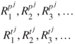
This then produces the time series of asset returns from ![]() :
:
Suppose these time series are normally distributed, as required by MPT. One can then calculate the means ![]() and
and ![]() and standard deviations
and standard deviations ![]() and
and ![]() , respectively.
, respectively.
According to MPT, the expected return on the investment is
subject to the constraint
where ![]() is a parameter to be found (see Adams et al. 2003): this parameter determines the proportion of
is a parameter to be found (see Adams et al. 2003): this parameter determines the proportion of ![]() devoted to poverty alleviation (
devoted to poverty alleviation (![]() ) and the proportion devoted to trade volume expansion (
) and the proportion devoted to trade volume expansion (![]() ).
).
Under the assumption of normally distributed asset returns
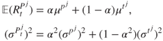
as the means ![]() and standard deviations
and standard deviations ![]() are constant in time.
are constant in time.
This situation has an optimal ‘risk-minimising’ solution when
This determines the ‘risk-minimising’ investment opportunity or, alternatively, the proportional investment in each possible asset which minimises the standard deviation of the total investment.
Then, aid usage is determined by investing ![]() in
in ![]() and
and ![]() in
in ![]() , thus maximising the expected rate of return while minimising the overall portfolio risk. The model is re-evaluated at each time step
, thus maximising the expected rate of return while minimising the overall portfolio risk. The model is re-evaluated at each time step ![]() .
.
16.3.6 Application
Continuing with Scenario 3, we apply the mechanism presented in Section 16.3.5. The initial aid allocation is shown in Figure 16.9 (![]() ). We supplement this data with the mean and variance of each asset for each recipient. Guided by recipient governance quality, given in Section 16.3.4, we assign these according to Table 16.1.
). We supplement this data with the mean and variance of each asset for each recipient. Guided by recipient governance quality, given in Section 16.3.4, we assign these according to Table 16.1.
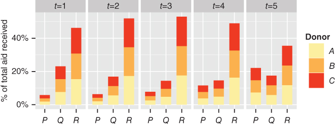
Figure 16.9 Aid allocation incorporating aid usage
Table 16.1 Parameters determining recipient investment
| Country | ||||
| P | 2 | 0.2 | 2 | 0.2 |
| Q | 0.5 | 0.5 | 0.5 | 0.7 |
| R | 0.5 | 0.7 | 0.5 | 0.7 |
Countries with lower governance quality ![]() are likely to lack the necessary bureaucratic infrastructure to successfully utilise development aid or lose aid to corruption throughout the investment process. Therefore, we associate a greater risk to countries with lower governance quality.1
are likely to lack the necessary bureaucratic infrastructure to successfully utilise development aid or lose aid to corruption throughout the investment process. Therefore, we associate a greater risk to countries with lower governance quality.1
Iterating the model forward from ![]() , aid allocation is as shown in Figure 16.9.
, aid allocation is as shown in Figure 16.9.
We see that ![]() is initially allocated the largest aid volume, reflecting its poverty headcount;
is initially allocated the largest aid volume, reflecting its poverty headcount; ![]() experiences its largest allocation at
experiences its largest allocation at ![]() , with diminishing subsequent allocations.
, with diminishing subsequent allocations. ![]() has the smallest initial allocation, which grows as the model is iterated forwards in time.
has the smallest initial allocation, which grows as the model is iterated forwards in time. ![]() has a middling initial allocation, which diminishes initially, reaching a nadir at
has a middling initial allocation, which diminishes initially, reaching a nadir at ![]() , but growing again thereafter.
, but growing again thereafter.
We can explain this situation by considering the changes resulting from recipient investment of aid (see Figure 16.10).
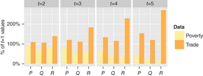
Figure 16.10 Poverty and trade levels of recipients following aid investment
Following the initial allocation, ![]() draws most aid. The investment parameters indicate (see Table 16.1) that
draws most aid. The investment parameters indicate (see Table 16.1) that ![]() invests equally in poverty reduction and trade expansion. However, having a significantly greater headcount than either
invests equally in poverty reduction and trade expansion. However, having a significantly greater headcount than either ![]() or
or ![]() ,
, ![]() continues to draw heavily from a donor community highly motivated by poverty.
continues to draw heavily from a donor community highly motivated by poverty.
![]() also splits its investment evenly between poverty reduction and trade expansion, but receives a relatively small aid volume compared to its comparator recipient nations. However, its fortunes begin to change after
also splits its investment evenly between poverty reduction and trade expansion, but receives a relatively small aid volume compared to its comparator recipient nations. However, its fortunes begin to change after ![]() has decreased its poverty headcount sufficiently for the governance advantage held by
has decreased its poverty headcount sufficiently for the governance advantage held by ![]() to become a determining factor in aid allocation; aid volumes increase significantly after
to become a determining factor in aid allocation; aid volumes increase significantly after ![]() .
.
![]() receives relatively little aid throughout, losing out initially to
receives relatively little aid throughout, losing out initially to ![]() and
and ![]() . However, as
. However, as ![]() 's aid allocation drops after
's aid allocation drops after ![]() ,
, ![]() begins to benefit. It is bias towards poverty reduction, as seen in investment parameters given in Table 16.1, mean its poverty headcount is reduced at a greater pace than trade expansion, which diminishes its likelihood of receiving aid in the subsequent time period.
begins to benefit. It is bias towards poverty reduction, as seen in investment parameters given in Table 16.1, mean its poverty headcount is reduced at a greater pace than trade expansion, which diminishes its likelihood of receiving aid in the subsequent time period.
16.3.7 Conclusions
Scenario 3 has shown how aid usage may be factored into a model of aid allocation, closing the counter-clockwise feedback loop of Figure 16.2 and feeding into donor preferences in allocation. Again, this process can produce complex outcomes.
While the approach sketched out earlier is clearly a heuristic, a stand-in for a full economic model encompassing the impact aid allocation on recipient economies, it does begin to encode behaviour identified in the literature.
16.4 Remarks
This Chapter presents a novel model of foreign aid allocation based on the mathematical theory of networks. Our intention is to capture the interconnected nature of this system, shedding light on the complex interactions between donors and recipients.
As we have shown, complex donor motivators in aid allocation can be described by our model. In particular, we have shown that heterogeneous donor motivation can lead to a wide variety of behaviours, even when donor nations share the same laudable intentions. Commercial and colonial relationships are shown to interact in an unpredictable manner with more altruistic, poverty-minded motivations.
Crucially, all allocations by our model are made in reference to the wider community of donors and recipients. This emphasises the increasingly networked nature of the global aid system which cannot be captured by more traditional dyadic analyses.
Our model allows for a simple characterisation of bandwagon behaviour (see Section 16.3.3). This characterisation is carried out in explicitly network theoretic terms and, hence, is an exploratory tool allowing connections not seen when using more traditional aid allocation models.
As we have shown, albeit in an exaggerated manner, bandwagon behaviour not only can skew the allocation of aid but can do so in an unexpected way in the context of our model. Over time, even a small tendency towards self-reinforcing behaviour can have a substantial impact upon the allocation of aid. This interaction becomes increasingly complex as the number of donor motivators increases.
This chapter joins an increasing chorus arguing that foreign aid should be viewed through the lens of complex systems analysis. Such a perspective suggests that aggregated data and assumptions in favour of homogeneity of motivation and behaviour are insufficient to describe global aid patterns. This chapter offers a new perspective on aid allocation and also suggests a new approach towards aid effectiveness using a conceptual-numerical modeling lens.
Acknowledgements
The authors thank R.G. Levy for a valuable tour of the development economics literature and the code used to generate the network images. A.G. Wilson and F.T. Smith provided helpful suggestions in developing this chapter. The authors acknowledge the financial support of the Engineering and Physical Sciences Research Council under the grant ENFOLDing—Explaining, Modelling, and Forecasting Global Dynamics, reference EP/H02185X/1.
References
- Adams, A.T., Booth, P.M., Bowie, D.C., and Freeth, D.S. (2003) Investment Mathematics, John Wiley & Sons, Ltd, Chichester.
- Alesina, A. and Dollar, D. (2000) Who gives foreign aid to whom and why? Journal of Economic Growth, 5 (1), 33–63.
- Balla, E. and Reinhardt, G.Y. (2008) Giving and receiving foreign aid: does conflict count? World Development, 36 (12), 2566–2585.
- Baulch, B. (2003) Aid for the poorest? The distribution and maldistribution of international development assistance. Chronic Poverty Research Centre (CPRC).
- Bermeo, S.B. (2008) Aid strategies of bilateral donors. Department of Political Science, Yale University. Unpublished manuscript.
- Berthélemy, J.C. (2006) Bilateral donors' interest vs. recipients' development motives in aid allocation: do all donors behave the same? Review of Development Economics, 10 (2), 179–194.
- Bhanumurthy, K. (2002) Arguing a case for the Cobb-Douglas production function. Review of Commerce Studies, 20, 21.
- Burnside, A.C. and Dollar, D. (2004) Aid, policies, and growth: revisiting the evidence. World Bank, Washington DC.
- Chong, A. and Gradstein, M. (2008) What determines foreign aid? The donors' perspective. Journal of Development Economics, 87 (1), 1–13.
- Cobb, C.W. and Douglas, P.H. (1928) A theory of production. The American Economic Review, 18 (1), 139–165.
- Collier, P. and Dollar, D. (2002) Aid allocation and poverty reduction. European Economic Review, 46 (8), 1475–1500.
- Dollar, D. and Levin, V. (2006) The increasing selectivity of foreign aid, 1984–2003. World Development, 34 (12), 2034–2046.
- Frot, E. and Santiso, J. (2011) Herding in aid allocation. Kyklos, 64 (1), 54–74.
- Fuchs, A., Dreher, A., and Nunnenkamp, P. (2014) Determinants of donor generosity: a survey of the aid budget literature. World Development, 56, 172–199.
- Gallo, G. (2013) Conflict theory, complexity and systems approach. Systems Research and Behavioral Science, 30 (2), 156–175.
- Harrigan, J. and Wang, C. (2011) A new approach to the allocation of aid among developing countries: is the USA different from the rest? World Development, 39 (8), 1281–1293.
- Hommes, C.H. (2006) Heterogeneous agent models in economics and finance. Handbook of Computational Economics, 2, 1109–1186.
- Marler, R.T. and Arora, J.S. (2004) Survey of multi-objective optimization methods for engineering. Structural and Multidisciplinary Optimization, 26 (6), 369–395.
- McBurney, P. (2012) What are models for? in Post-Proceedings of the 19th European Workshop on Multi-Agent Systems (EUMAS 2011), Lecture Notes in Computer Science, vol. 7541 (eds M. Cossentino, K. Tuyls, and G. Weiss) Springer-Verlag, Berlin, pp. 175–188.
- McGillivray, M. (2003) Modelling aid allocation: issues, approaches and results, 2003/49, WIDER Discussion Papers//World Institute for Development Economics (UNU-WIDER).
- McGillivray, M. (2004) Descriptive and prescriptive analyses of aid allocation: approaches, issues, and consequences. International Review of Economics & Finance, 13 (3), 275–292.
- McGillivray, M. (2006) Aid allocation and fragile states, in Fragile States: Causes, Costs and Responses (eds W. Naudé, A.U. Santos-Paulino, and M. McGillivray), Oxford University Press, Oxford, pp. 166–184.
- Newman, M. (2010) Networks: An Introduction, Oxford University Press, Oxford.
- Ramalingam, B. (2011) Aid on the Edge of Chaos, Oxford University Press, Oxford.
- Riddell, R.C. (2007) Does Foreign Aid Really Work? Oxford University Press, Oxford.
- Schelling, T.C. (1971) Dynamic models of segregation. Journal of Mathematical Sociology, 1 (2), 143–186.
- Schiller, R.J. (2000) The irrational exuberance. Princeton University Press, Princeton.
- Simon, H.A. and Levy, F.K. (1963) A note on the Cobb-Douglas function. The Review of Economic Studies, 30 (2), 93–94.
- Tarp, F., Bach, C.F., Hansen, H., and Baunsgaard, S. (1999) Danish Aid Policy: Theory and Empirical Evidence, Springer-Verlag, Heidelberg.
- United Kingdom Government (2002) International Development Act 2002 1(1)a.
- United States Government (1961) Foreign Assistance Act of 1961 Sec. 101(a).
- Wilson, A. (2012) The Science of Cities and Regions, Springer-Verlag, Berlin.
- Younas, J. (2008) Motivation for bilateral aid allocation: altruism or trade benefits. European Journal of Political Economy, 24 (3), 661–674.
Appendix
A.1 Common Functional Definitions
Common functional definitions are collected in this appendix. Variables not discussed here may be assumed to be easily defined from Section 16.2.5.
| Variable | Definition |
| Colonial relationship between donor
|
|
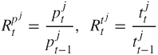
Prior success in receiving aid, the total volume of aid received in the previous year, |