
Chapter 10
Rebellions
Peter Baudains, Jyoti Belur, Alex Braithwaite, Elio Marchione and Shane D. Johnson
10.1 Introduction
Rebellions frequently arise around the globe and have received considerable attention from the academic community. Data-driven studies have traditionally analysed such civil conflicts at the country-year level (e.g. Gurr, 1970; Fearon and Laitin, 2003) and rarely explicitly model the interaction between rebels and the state (although there are notable exceptions, such as Toft and Zhukov, 2012, 2015). In this chapter, we contribute to an emerging literature on the temporal dynamics of rebellions by using a point process framework to model the evolution of the Naxal rebellion within the Indian state of Andhra Pradesh at a daily level of resolution. We model the occurrence of Naxal attacks and police counterinsurgent actions as a coupled point process, which enables us to consider the level of interaction between the two sides of the conflict.
The Naxal movement, whose name is taken from the small village of Naxalbari in West Bengal, where a peasant revolt took place in 1967, is a left-wing extremist group who have engaged in numerous attacks against civilians and the state in recent decades. Grievances of the Naxal movement initially stemmed from economic inequality and rural agricultural workers' inaccessibility to land ownership (Ahuja and Ganguly, 2007). After being quashed by the Indian government in the 1970s through the use of police and paramilitary forces (Basu, 2011), several factions of the Naxal movement were formed, many of which had militant groups who engaged in insurgency against the state. In the early 2000s, various Naxal groups merged to form both militant (the People's Liberation Guerrilla Army) and political groups (the Communist Party of India (Maoist)). Insurgent violence continues to present day, but, in recent years, tends to be restricted within localised regions in Eastern and North Eastern India.
The states of Andhra Pradesh and Telangana, the latter of which was formed in 2014 when Andhra Pradesh bifurcated, experienced high levels of violence during the 2000s. Police periodically adopted various counterinsurgency measures in an attempt to quell the rebellion, including the formation of an aggressive paramilitary group called the Greyhounds. On numerous occasions, the police were drawn into armed conflict with the rebels, resulting in both Naxal and police loss of life. Police counterinsurgent measures in Andhra Pradesh have been claimed to be effective in reducing levels of violence, despite limited quantitative studies (Sahni, 2007).
In this chapter, we analyse the temporal dynamics associated with the Naxal rebellion, using data on insurgent actions and counterinsurgent response. We employ a multivariate Hawkes process model and investigate how the rebellion changed by comparing parameter estimates and overall model fit for two time periods. Our findings identify differences in the dynamics of the rebellion as it evolved. The time periods considered fall on either side of a reported truce on the part of the police, which was called in response to the formation of the Communist Party of India (Maoist) in the hope that a diplomatic solution to the insurgency could be found. However, no solution was forthcoming and insurgent attacks continued, which led, eventually, to a resumed counterinsurgent campaign. We discuss how the temporal dynamics changed between the two time periods, considering any potential effect of this truce.
We begin by outlining the data used in this chapter and explain why it is of interest to consider distinct time periods before presenting the multivariate Hawkes process model. Similar models have recently been used to model a wide range of different temporal dynamics, including, in many cases, the occurrence of events related to crime and security. We outline how the parameters in the model can be obtained from the data using a maximum-likelihood procedure and explain how they might be interpreted. We then present the results for the two time periods considered. These consist of the maximum-likelihood parameter estimates associated with each of the two time periods, bootstrapped distributions for each of those estimates and also a residual analysis to examine overall model fit. We conclude by discussing the implications of these findings with respect to our understanding of the Naxal movement and to rebellions more generally.
10.2 Data
Police recorded crime data detailing hostile events associated with the Naxal rebellion for the 10-year period 2000–2010 in the state of Andhra Pradesh were provided by the Andhra Pradesh police. The data consisted of official police records of Naxal-related violence or threat recorded in the 1,642 police stations within the state. Counterinsurgent activities of police were not detailed explicitly in the data; however, fieldwork described in Belur (2010) and subsequent fieldwork conducted in left wing extremist affected areas suggests that aggressive police action took place and sometimes involved the killing of unwanted persons (in this case Naxals) during shootouts. Such events were recorded as an “exchange of fire” in the data. As a result, it is assumed that events described in the dataset as an “exchange of fire” between Naxal and police, and which resulted in at least one Naxal fatality, were largely caused by strategic counterinsurgency activities. On this basis, it is possible to partition the data set into events initiated by Naxals and events initiated by police.
The temporal distribution of the 4,820 incidents in the data set is shown in Figure 10.1, where the shading of each bar indicates the number of events that occur each week (darker shading corresponds to more events). This figure also distinguishes between the 4,234 Naxal events (in red) and the 586 police events (in blue). In what follows, we analyse the temporal dependence between these two sets of events. In particular, we examine the extent to which the temporal signatures of these events exhibit self- or mutually exciting dynamics with a multivariate Hawkes process.
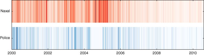
Figure 10.1 Temporal distribution of the event data
As shown in Figure 10.1, midway through 2004, no police actions were identified for a period of around 6 months. This period coincides with a reported cease fire adopted by the Indian police. The number of Naxal attacks during this period does not have a similar reduction, and Figure 10.1 suggests that they may have even increased.
To examine the effect that this truce had on the dynamics of the insurgency, and in an attempt to set up a natural experiment, we split the data to be examined into two distinct time periods. The first, from the beginning of the data set on 1 January 2000 to 31 December 2003, contains the period of time before the truce and during which the conflict was at its most intense. Although the truce did not begin until May 2004, we truncate the first time period to 31 December 2003 to discount any dynamics in the build up to this truce. The second time period is taken to start once police actions resume after the truce on 1 January 2005. To ensure that the two time periods are of the same length, the second interval is taken to end on 31 December 2008. In what follows, we explain the model to be applied to these two time periods before calibrating it on them separately. We compare the results obtained and discuss any differences that arise.
10.3 Hawkes model
A number of studies have investigated the timings of events associated with issues in crime and security using a point process modelling framework. A wide range of structural variables can be incorporated into a point process model; however, recent examples have typically only included information on the timing of historic events. The reason for this is that many types of events, such as urban crime (e.g. Pease, 1998; Johnson et al., 2007) and insurgency (Townsley et al., 2008), have been shown to cluster in both space and time. In other words, the timing of one event often signals an elevation or “excitation” in the risk of others in the near future. For example, Holden 1986 uses the so-called Hawkes process (Hawkes, 1971), which accounts, for excitation in the rate at which events occur, to determine whether a contagion effect can be observed in the frequency of aircraft hijackings in the United States between 1968 and 1972. More recently, Hawkes processes have been employed to model the timings of events associated with gang rivalries (Egesdal et al., 2010) and civilian deaths during the Iraq war (Lewis et al., 2011). Extensions of this same model have also been used to consider the timings of terrorist attacks in Southeast Asia (Porter and White, 2012; White et al., 2013). Short et al. 2014 propose a multivariate point process model to account for possible interaction effects arising from the behaviours of different gangs. Spatio-temporal models of point processes, in which the locations as well as the timings of future events are modelled, have been used to model burglary (Mohler et al., 2011) and insurgent warfare (Zammit-Mangion et al., 2012). Such studies demonstrate that, when calibrated, point process models can generate more accurate predictions than contending alternatives.
We define a point process as a collection of random events ![]() ordered so that
ordered so that ![]() , where
, where ![]() denotes the time at which event
denotes the time at which event ![]() occurred and
occurred and ![]() is a component index. A point process is simple if this inequality is strict for all values of
is a component index. A point process is simple if this inequality is strict for all values of ![]() . In the present study,
. In the present study, ![]() denotes an event initiated by Naxals and
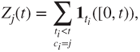
denotes an event initiated by Naxals and ![]() denotes an event initiated by police. If the timings of events for each component is modelled as a separate process, as will be the case in the models that follow, then the point process is multivariate. More formally, a multivariate point process is defined as a series of counts
denotes an event initiated by police. If the timings of events for each component is modelled as a separate process, as will be the case in the models that follow, then the point process is multivariate. More formally, a multivariate point process is defined as a series of counts
on some temporal domain ![]() (for some maximum time
(for some maximum time ![]() ) defined by
) defined by
where ![]() is an indicator function, which is equal to one if
is an indicator function, which is equal to one if ![]() and equal to zero otherwise. The subscript
and equal to zero otherwise. The subscript ![]() is used to denote the type of event (with
is used to denote the type of event (with ![]() denoting Naxals and
denoting Naxals and ![]() denoting police).
denoting police).
The history of the system until some time ![]() ,
, ![]() , is defined to be the set of events that have occurred before time
, is defined to be the set of events that have occurred before time ![]() , so that
, so that
The conditional intensity function associated with the count ![]() is defined as
is defined as
For a given ![]() , if
, if ![]() is simple and finite for all
is simple and finite for all ![]() , then the associated conditional intensity function
, then the associated conditional intensity function ![]() is unique (Daley and Vere-Jones, 2003). It follows that in order to define a particular simple and finite point process given by
is unique (Daley and Vere-Jones, 2003). It follows that in order to define a particular simple and finite point process given by ![]() , it is sufficient to specify the function
, it is sufficient to specify the function ![]() . Many models of point processes specify a functional form for the conditional intensity function, rather than for the count, and this is also the approach that is taken here.
. Many models of point processes specify a functional form for the conditional intensity function, rather than for the count, and this is also the approach that is taken here.
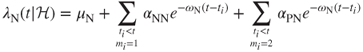
We employ a two-dimensional Hawkes process with conditional intensity functions for the Naxal events, ![]() , and police events,
, and police events, ![]() , given by
, given by

for parameters ![]() ,
, ![]() ,
, ![]() and
and ![]() , which describe the way in which the rate of Naxal attacks depends on the history of the system, and for parameters
, which describe the way in which the rate of Naxal attacks depends on the history of the system, and for parameters ![]() ,
, ![]() ,
, ![]() and
and ![]() , which describe the way in which the rate of police events depends on the history of the system.
, which describe the way in which the rate of police events depends on the history of the system.
The Hawkes models in Equations (10.5) and (10.6) suppose that events arise as a result of two possible processes: a background rate, which is modelled as a Poisson process with constant intensity, and excitation, which is modelled as a sum of terms that exponentially decay with the time from each event.
Background events are supposed to occur naturally throughout the duration of study with constant intensity. In the case of the Naxals, the rate of background events might indicate some baseline level of underlying grievances over the time period studied, where these grievances are equally likely to result in attacks at any point in time. In the case of the police, background events might occur due to a consistent policy directed to ensure a certain number of counterinsurgent operations take place in a given time frame. The parameters ![]() and
and ![]() define the background rate of the Naxal and police processes, respectively.
define the background rate of the Naxal and police processes, respectively.
Excitation arises when a number of events occur more closely together than is considered to be plausibly represented by a constant Poisson process. As a result, these terms account for any temporal clustering in the process. In Equations (10.5) and (10.6), the occurrence of either type of event can contribute to an increase in the intensity functions. The magnitude of this increase is determined by the parameters ![]() , when Naxal events cause an increase in the Naxal intensity function;
, when Naxal events cause an increase in the Naxal intensity function; ![]() , when a police event causes an increase in the Naxal intensity function;
, when a police event causes an increase in the Naxal intensity function; ![]() , when a Naxal event causes an increase in the police intensity function; and
, when a Naxal event causes an increase in the police intensity function; and ![]() , when police events increase the police intensity function. The decay terms
, when police events increase the police intensity function. The decay terms ![]() and
and ![]() describe the rate at which this increased excitation decays, with higher values representing a more rapid decline in excitation.
describe the rate at which this increased excitation decays, with higher values representing a more rapid decline in excitation.
Temporal clustering of events—which the excitation terms in Equations (10.5) and (10.6) are designed to capture—can arise as a result of a number of mechanisms. It may be that the occurrence of an event directly influences the chance of further events occurring. In the case of the Naxals, this can arise if insurgents are inspired to carry out further attacks once they have observed or taken part in a successful attack (Johnson and Braithwaite, 2009). Similarly, responding to prior police events, insurgents might retaliate as a direct result of police action. Indeed, tit-for-tat behaviour between opponents during insurgencies has been identified in a number of previous studies (Linke et al., 2012; O'Loughlin and Witmer, 2012; Braithwaite and Johnson, 2012). Clustering may also arise as a result of confounding factors that make certain time periods more likely to experience events, creating risk heterogeneity in time. For example, improved communication or a change in leadership within the rebellion group might coincide with an increase in the rate of attacks. This type of clustering can produce similar patterns in the event data to self-excitation and it can be difficult to disentangle the causal effect (Mohler, 2013).
In a similar way to insurgent attacks, clustering of police actions can be caused, on the one hand, by prior events (e.g. police may retaliate to Naxal attacks or be more incentivised to undertake further action after successful police actions) or, on the other, by confounding factors that generate risk heterogeneity (e.g. if the police are adhering to a recently introduced policy supporting the increased rate of counterinsurgent activity).
The Hawkes process does not distinguish between explanations of temporally varying factors and direct excitation; instead, only distinguishing between time-stable factors that might influence the rate of attacks—as described by the background rate—and the change in risk intensity due to clustering that is modelled as excitation. Nevertheless, the model is useful for a number of reasons. First, it can be used to identify temporal regularities in the data, which may then be studied further to consider the causal mechanisms that might be responsible. Second, the model can quantify the rate with which events are occurring in a given period, which can be used for assessing the severity of the disorder or assessing whether responses to any violence were appropriate. Third, the model is well suited to prediction: clustering of recent events can indicate whether events are more or less likely to occur in the future.
Parameter estimates can be obtained via a maximum-likelihood procedure. The log-likelihood function for the multivariate process in Equations (10.5) and (10.6) is given by

where ![]() denotes the end point of the time period of interest (Embrechts et al., 2011). The parameters
denotes the end point of the time period of interest (Embrechts et al., 2011). The parameters ![]() and
and ![]() that maximise the value of the function in Equation (10.7) are the parameters that most closely fit the models in Equations (10.5) and (10.6) to the data.
that maximise the value of the function in Equation (10.7) are the parameters that most closely fit the models in Equations (10.5) and (10.6) to the data.
The uncertainty of the parameters ![]() and
and ![]() can be estimated via a parametric bootstrap procedure (Wang et al., 2010). This is performed by simulating a large number of histories of a system defined by the models in Equations (10.5) and (10.6), specified with the parameters as obtained from the maximum likelihood procedure. For each simulated history, the parameters are then re-estimated. If these values are consistently close to the parameters estimated from the data, then there is confidence that those parameters specify a model that is close to what is observed. If there is a large range in re-estimated parameter values from these simulated processes, then the observed process might have been plausibly reproduced with quite different parameters, therefore indicating greater uncertainty.
can be estimated via a parametric bootstrap procedure (Wang et al., 2010). This is performed by simulating a large number of histories of a system defined by the models in Equations (10.5) and (10.6), specified with the parameters as obtained from the maximum likelihood procedure. For each simulated history, the parameters are then re-estimated. If these values are consistently close to the parameters estimated from the data, then there is confidence that those parameters specify a model that is close to what is observed. If there is a large range in re-estimated parameter values from these simulated processes, then the observed process might have been plausibly reproduced with quite different parameters, therefore indicating greater uncertainty.
While the bootstrap procedure enables the assessment of uncertainty in the model at the parameter level, a residual analysis can be used to determine how well the model fits the data overall. A residual process is obtained by probabilistically selecting events from the data set that occur when the modelled intensity is at its lowest. This process therefore selects events that were poorly predicted by the model (i.e. such events represent a departure between the model and the data that it attempts to recreate). If the model is a good fit to the data, then the residual events would be expected to form a Poisson process over the study period. Considering the extent to which the residual process deviates from a Poisson process, therefore, indicates the goodness of fit of the model.
In the next section, results are presented for two time periods during the Naxal rebellion. These results consist of point estimates for the models proposed in Equations (10.5) and (10.6); the distribution of these estimates as obtained from the bootstrap procedure; and the comparison between the residual processes obtained for each time period, compared to a constant Poisson process. The results provide a number of insights into the nature of the rebellion and these are then discussed.
10.4 Results
The vectors ![]() and
and ![]() that maximise 1 the log-likelihood over the two time periods and which therefore most closely fit the model in Equations (10.5) and (10.6) are shown in Table 10.1. When calculating these estimates, a randomisation procedure was performed on concurrent events, whereby a random time interval of less than 1 day is added to each event that occurs on the same day. This is performed to ensure that the data form a simple point process (with no two events occurring at the exact same point in time), thereby ensuring the uniqueness of the conditional intensity function. Although the procedure to remove concurrent events was random, meaning that slightly different event histories could be used to calibrate the parameters over repeated optimisations, there was very little variance in the optimal parameters obtained across 20 such procedures. The results reported are the means from these 20 optimisation procedures.
that maximise 1 the log-likelihood over the two time periods and which therefore most closely fit the model in Equations (10.5) and (10.6) are shown in Table 10.1. When calculating these estimates, a randomisation procedure was performed on concurrent events, whereby a random time interval of less than 1 day is added to each event that occurs on the same day. This is performed to ensure that the data form a simple point process (with no two events occurring at the exact same point in time), thereby ensuring the uniqueness of the conditional intensity function. Although the procedure to remove concurrent events was random, meaning that slightly different event histories could be used to calibrate the parameters over repeated optimisations, there was very little variance in the optimal parameters obtained across 20 such procedures. The results reported are the means from these 20 optimisation procedures.
Table 10.1 Point estimates for parameters in Equations (10.5) and (10.6). The calibration is performed separately for two different time periods
| Time interval | ||||||||
| 2000–2003 | 0.5992 | 0.6054 | 0.0000 | 0.1592 | 0.0424 | 0.5684 | 0.0390 | 0.0633 |
| 2005–2008 | 0.0851 | 0.7461 | 0.8790 | 0.1394 | 0.0442 | 0.2528 | 0.0718 | 0.0599 |
The point estimates in Table 10.1 show some striking differences between the two time periods, but there are also a number of similarities. The decay rates, given by ![]() and
and ![]() , are found to be quite similar for the two time periods. Any increased intensity due to the occurrence of events is estimated to decay over a period of around
, are found to be quite similar for the two time periods. Any increased intensity due to the occurrence of events is estimated to decay over a period of around ![]() days in the case of Naxal events and around
days in the case of Naxal events and around ![]() days in the case of police events. The background rate for police events,
days in the case of police events. The background rate for police events, ![]() , is also similar over the two time periods considered. Around 0.04 police background events are expected to occur each day on average.
, is also similar over the two time periods considered. Around 0.04 police background events are expected to occur each day on average.
Background Naxal events occur with a rate of around 0.6 between 2000 and 2003 and with a rate of around 0.09 between 2005 and 2008, signifying quite a departure from the dynamics over the first time period. Perhaps to account for this severe reduction, excitation of Naxal events from both Naxal and police events is found to be much greater during the second time period considered. During the first time period, no excitation effect is found from police events on the Naxal intensity function, but quite a large excitation is observed in the second time interval.
The excitation of police events also varies over the two time intervals considered, although not to such a large extent. The size of self-excitation of police events decreases in the second time interval from the first, but retaliation from Naxal events increases.
The results in Table 10.1 are just point estimates and so, in order to determine the level of uncertainty associated with them, we plot the density of the distribution of bootstrap estimates for each parameter for 2000–2003 and for 2005–2008 in Figure 10.2. These densities are constructed by re-estimating the parameters from a simulation of the model in Equations (10.5) and (10.6), specified with the parameters in Table 10.1, a process which is repeated 100 times. The point estimates for each time interval are plotted by a dashed line in each case. By examining these figures, it is possible to determine the degree of uncertainty associated with each estimate. If the distribution of bootstrap estimates spans a wide region on the ![]() -axis of each figure, then there is a large uncertainty associated with the corresponding point estimate. If, on the other hand, the density plot only covers quite a small region and has a well-defined and sharp maximum, then there is low uncertainty associated with the estimate.
-axis of each figure, then there is a large uncertainty associated with the corresponding point estimate. If, on the other hand, the density plot only covers quite a small region and has a well-defined and sharp maximum, then there is low uncertainty associated with the estimate.

Figure 10.2 The distribution of each parameter, as obtained from the bootstrap procedure, for the period 2000–2003 (in blue) and 2005–2008 (in red). The shaded distributions are density plots obtained from 100 re-estimations of the parameters from simulations of the process in Equations (10.5) and (10.6). The dashed lines represent the point estimates in Table 10.1 and correspond to the parameters with which these simulations are specified
The distributions of the parameter values obtained from the bootstrap procedure are, on the whole, consistent with the point estimates. A number of the distributions appear to be truncated at zero, as can be detected by the smaller local peak on the left of the global maximum in a number of the distributions. This suggests that, in these cases, the parameters are likely to be indistinguishable from zero or from very small positive values. In addition, there appears to be greater uncertainty associated with the parameters of ![]() than the parameters of
than the parameters of ![]() for both time periods, perhaps owing to the relatively smaller number of police events in comparison to Naxal events.
for both time periods, perhaps owing to the relatively smaller number of police events in comparison to Naxal events.
A number of the conclusions made above with regard to the differences between the two time intervals are supported by the distributions in Figure 10.2. For ![]() , the lack of any intersection in the two distributions supports the finding that the background rate of Naxal attacks decreased in the second time period. The distributions for
, the lack of any intersection in the two distributions supports the finding that the background rate of Naxal attacks decreased in the second time period. The distributions for ![]() and
and ![]() are consistent with the finding that excitation of the Naxal intensity function increased in the second time period, although the distributions do intersect over a small interval. The remaining parameters have distributions that intersect over quite a wide range of their possible values, although the modal values in the density plots are consistent with the change identified in the point estimates (with the exception of
are consistent with the finding that excitation of the Naxal intensity function increased in the second time period, although the distributions do intersect over a small interval. The remaining parameters have distributions that intersect over quite a wide range of their possible values, although the modal values in the density plots are consistent with the change identified in the point estimates (with the exception of ![]() ; although very little change in the point estimates was identified in this case).
; although very little change in the point estimates was identified in this case).
In order to determine the overall model fit, comparison of the residual process against a Poisson process is made in two QQ-plots in Figure 10.3. This figure is constructed by randomly simulating 1,000 residual processes of length 107 for the model of both Naxal and police events in Equations (10.5) and (10.6), using the parameters in Table 10.1 for the two time periods under consideration. Length 107 is chosen since this would be the expected number of Poisson distributed events (of both types) as calculated by the smaller of the background rates for the two periods (the second time period being the smallest). For each quantile value on the ![]() -axis, the proportion of events in each residual process remaining is calculated, and the 95% confidence interval of these values is plotted against what would be expected assuming a Poisson process. Thus, the black lines in Figure 10.3 represent the 95% confidence of the residual process compared against a Poisson process. The grey shaded region plots what would be observed if the process was exactly a Poisson process.
-axis, the proportion of events in each residual process remaining is calculated, and the 95% confidence interval of these values is plotted against what would be expected assuming a Poisson process. Thus, the black lines in Figure 10.3 represent the 95% confidence of the residual process compared against a Poisson process. The grey shaded region plots what would be observed if the process was exactly a Poisson process.
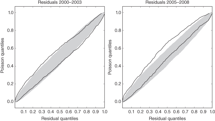
Figure 10.3 QQ-plots comparing the residual process to a Poisson process for the two time periods. The black lines represent the 95% confidence interval of the quantiles of the residual process in comparison to a Poisson process. These are obtained from 1,000 samples of the residual process. The grey shaded region represents an equivalent Poisson process
The model fit is considered to be good if the residual process resembles a Poisson process, and thus if the black lines in Figure 10.3 lie within the grey shaded region. The process associated with the first time interval lies more closely within the grey shaded region than the second time interval and so we conclude that the model fits the first time period better overall.
10.5 Discussion
In this chapter, we have examined the temporal dynamics associated with the Naxal rebellion and the police response to it. We fitted a multivariate Hawkes process to events associated with both Naxal insurgent attacks and police counterinsurgent actions to two periods on either side of a truce undertaken by the police. For both periods, evidence was found for self-excitation of both Naxal and police events: Naxal events increased the likelihood of further Naxal events and police events increased the likelihood of further police events. In the second time period, the strength of self-excitation was increased for Naxal events and decreased for police events. The second time interval appeared to contain higher levels of mutual excitation: police actions increased the likelihood of Naxal attacks and vice versa and more so in the second period than in the first. In addition, the background rate of Naxal attacks decreased significantly in the second period.
The sensitivity of these findings has been explored via a bootstrap procedure to obtain an indication of parameter uncertainty, as well as by employing a residual process to ascertain overall model fit. When interpreting these findings, it should be borne in mind that the model fits the data better in the first time interval, when more of the events can be attributed to the background process, than in the second time interval, in which excitation appears to be more dominant.
Despite limitations associated with the sensitivity of the model, our findings suggest that the second time interval had distinct dynamics from the first. There were fewer events (as can be seen from Figure 10.1), but they tended to be more susceptible to clustering via excitation processes. There are a number of mechanisms that might account for this pattern. It may be that the grievances of the Naxals were, on the whole, much reduced in the second time interval, but that sporadic outbursts of events arose in response to a particular counterinsurgent action or other policy aimed at the insurgents. The increased clustering of events during the second time period is consistent with a smaller but more organised insurgent campaign, which seeks to maximise impact by committing a number of attacks in a short period of time (Johnson and Braithwaite, 2009). These regularities might also be explained by an effective counterinsurgent campaign, which reduced the likelihood of events for the majority of the second time interval, but which suffered periodic setbacks in the form of a number of closely clustered attacks.
Despite uncertainty with respect to the causal mechanisms, the pattern identified in this exploratory approach can help stimulate further, more detailed analysis. Further work might investigate the differences identified and construct models that directly incorporate causal mechanisms and structural covariates. Baudains 2015 disaggregates the model presented here to incorporate geography and examine the resulting spatial excitation. He also utilises a predictive analysis to determine the extent to which regularities in the data might be used as a predictive tool. This demonstrates how point process frameworks might be used in a policy setting (see also Zammit-Mangion et al., 2012; Mohler et al., 2011).
In conclusion, we have shown that regularities exist within the social dynamics of rebellions that can be exploited in a statistical framework to obtain insights. Importantly, using the history of the system as the only data in the model has generated these insights, highlighting the utility of the point process framework. Our findings emphasise the increased prominence of excitation as the conflict progressed. In addition to self-excitation, we conclude that mutual excitation plays an important role, indicating the presence of retaliation or tit-for-tat behaviour, particularly during the latter stages of the insurgency. The analysis of other rebellions using a similar framework might further improve our understanding of these types of social dynamics.
References
- Ahuja, P. and Ganguly, R. (2007) The fire within: naxalite insurgency violence in India. Small Wars and Insurgencies, 18 (2), 249–274.
- Basu, I. (2011) Security and development - are they two sides of the same coin? Investigating India's two-pronged policy towards left wing extremism. Contemporary South Asia, 19 (4), 373–393.
- Baudains, P.J. (2015) Spatio-temporal modelling of civil violence: four frameworks for obtaining policy-relevant insights. Doctoral Dissertation, University College London, London.
- Belur, J. (2010) Permission to Shoot? Police Use of Deadly Force in Democracies, Springer-Verlag, New York.
- Braithwaite, A. and Johnson, S.D. (2012) Space-time modeling of insurgency and counter-insurgency in Iraq. Journal of Quantitative Criminology, 28 (1), 31–48.
- Daley, D. and Vere-Jones, D. (2003) An Introduction to the Theory of Point Processes, Volume I: Elementary Theory and Methods in Applied Sciences, No. 1, 2nd edn, Springer-Verlag, New York, pp. 114–122.
- Egesdal, M., Fathauer, C., Louie, K., and Neuman, J. (2010) Statistical and stochastic modeling of gang rivalries in Los Angeles. SIAM Undergraduate Research Online, 3, 72–94.
- Embrechts, P., Liniger, T., and Lin, L. (2011) Multivariate Hawkes processes: an application to financial data. Journal of Applied Probability, 48, 367–378.
- Fearon, J.D. and Laitin, D.D. (2003) Ethnicity, insurgency, and civil war. American Political Science Review, 97 (1), 75.
- Gurr, T. (1970) Why Men Rebel, Princeton University Press, Princeton, NJ.
- Hawkes, A.G. (1971) Spectra of some self-exciting and mutually exciting point processes. Biometrika, 58 (1), 83–90.
- Holden, R.T. (1986) The contagiousness of aircraft hijacking. American Journal of Sociology, 91 (4), 874–904.
- Johnson, S.D., Bernasco, W., Bowers, K.J., Elffers, H., Ratcliffe, J., Rengert, G., and Townsley, M. (2007) Space-time patterns of risk: a cross national assessment of residential burglary victimization. Journal of Quantitative Criminology, 23, 201–219.
- Johnson, S.D. and Braithwaite, A. (2009) Spatio-temporal distribution of insurgency in Iraq, in Countering Terrorism through SCP, Crime Prevention Studies, vol. 25 (eds J.D. Freilich and G.R. Newman), Criminal Justice Press, New York, pp. 9–32.
- Lewis, E., Mohler, G., Brantingham, P.J., and Bertozzi, A.L. (2011) Self-exciting point process models of civilian deaths in Iraq. Security Journal, 25 (3), 244–264.
- Linke, A.M., Witmer, F.D., and O'Loughlin, J. (2012) Space-time granger analysis of the war in Iraq: a study of coalition and insurgent action-reaction. International Interactions, 38 (4), 402–425.
- Mohler, G. (2013) Modeling and estimation of multi-source clustering in crime and security data. The Annals of Applied Statistics, 7 (3), 1525–1539.
- Mohler, G.O., Short, M.B., Brantingham, P.J., Schoenberg, F.P., and Tita, G.E. (2011) Self-exciting point process modeling of crime. Journal of the American Statistical Association, 106 (493), 100–108.
- Nelder, J.A. and Mead, R. (1965) A simplex method for function minimization. The Computer Journal, 7, 308–313.
- O'Loughlin, J. and Witmer, F.D. (2012). The diffusion of violence in the North Caucasus of Russia, 1999–2010. Environment and Planning A 44: 2379–2396.
- Pease, K. (1998). Repeat victimization: taking stock. The Home Office: Police Research Group: Crime Detection and Prevention Series Paper 90.
- Porter, M.D. and White, G. (2012) Self-exciting hurdle models for terrorist activity. The Annals of Applied Statistics, 6 (1), 106–124.
- Sahni, A. (2007) Andhra Pradesh: the state advances, the Maoists retreat. South Asia Intelligence Review: Weekly Assessments and Briefings, 6 (10), 1.
- Short, M.B., Mohler, G.O., Brantingham, P.J., and Tita, G.E. (2014) Gang rivalry dynamics via coupled point process networks. Discrete and Continuous Dynamical Systems - Series B, 19 (5), 1459–1477.
- Toft, M.D. and Zhukov, Y.M. (2012) Denial and punishment in the North Caucasus: evaluating the effectiveness of coercive counter-insurgency. Journal of Peace Research, 49 (6), 785–800.
- Toft, M.D. and Zhukov, Y.M. (2015) Islamists and Nationalists: rebel motivation and counterinsurgency in Russia's North Caucasus. American Political Science Review, 109 (2), 222–238.
- Townsley, M., Johnson, S.D., and Ratcliffe, J.H. (2008) Space time dynamics of insurgent activity in Iraq. Security Journal, 21 (3), 139–146.
- Wang, Q., Schoenberg, F.P., and Jackson, D.D. (2010) Standard errors of parameter estimates in the ETAS Model. Bulletin of the Seismological Society of America, 100 (5A), 1989–2001.
- White, G., Porter, M.D., and Mazerolle, L. (2013) Terrorism risk, resilience and volatility: a comparison of terrorism patterns in three Southeast Asian countries. Journal of Quantitative Criminology, 29 (2), 295–320.
- Zammit-Mangion, A., Dewar, M., Kadirkamanathan, V., and Sanguinetti, G. (2012) Point process modelling of the Afghan War Diary. Proceedings of the National Academy of Sciences of the United States of America, 109 (31), 12414–12419.