2
Continuous‐Domain Signals and Systems
2.1 Introduction
This chapter presents the relevant theory of continuous‐domain signals and systems, mainly as it applies to still and time‐varying images. This is a classical topic, well covered in many texts such as Papoulis's treatise on Systems and Transforms with Applications in Optics [Papoulis (1968)] and the encyclopedic Foundations of Image Science [Barrett and Myers (2004)]. The goal of this chapter is to present the necessary material to understand image acquisition and reconstruction systems, and the relation to discrete‐domain signals and systems. Fine points of the theory and vastly more material can be found in the cited references.
A continuous‐domain planar time‐varying image ![]() is a function of two spatial dimensions
is a function of two spatial dimensions ![]() and
and ![]() , and time
, and time ![]() , usually observed in a rectangular spatial window
, usually observed in a rectangular spatial window ![]() over some time interval
over some time interval ![]() . In the case of a still image,
. In the case of a still image, ![]() has a constant value for each
has a constant value for each ![]() , independently of
, independently of ![]() . In this case, we usually suppress the time variable, and write
. In this case, we usually suppress the time variable, and write ![]() . We use a vector notation
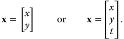
. We use a vector notation ![]() to simplify the notation and handle two and three‐dimensional (and higher‐dimensional) cases simultaneously. Thus
to simplify the notation and handle two and three‐dimensional (and higher‐dimensional) cases simultaneously. Thus ![]() is understood to mean
is understood to mean ![]() in the two‐dimensional case and
in the two‐dimensional case and ![]() in the three‐dimensional case. We will denote
in the three‐dimensional case. We will denote ![]() and
and ![]() , where
, where ![]() is the set of real numbers. To cover both cases, we write
is the set of real numbers. To cover both cases, we write ![]() , where normally
, where normally ![]() or
or ![]() ; also the one‐dimensional case is covered with
; also the one‐dimensional case is covered with ![]() and most results apply for dimensions higher than 3. For example, the domain for time‐varying volumetric images is
and most results apply for dimensions higher than 3. For example, the domain for time‐varying volumetric images is ![]() . It is often convenient to express the independent variables as a column matrix, i.e.
. It is often convenient to express the independent variables as a column matrix, i.e.
Since there is no essential difference between ![]() and the space of
and the space of ![]() column matrices, we do not distinguish between these different representations. We will often abbreviate two‐dimensional as 2D and three‐dimensional as 3D.
column matrices, we do not distinguish between these different representations. We will often abbreviate two‐dimensional as 2D and three‐dimensional as 3D.
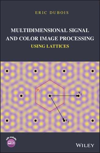
The spatial window ![]() is of dimensions
is of dimensions ![]() where pw is the picture width and ph is the picture height. Since the absolute physical size of an image depends on the sensor or display device used, we often choose to adopt the ph as the basic unit of spatial distance, as has long been common in the broadcast video industry. However, we are free to choose any convenient unit of length in a given application, for example, the size of a sensor or display element, or an absolute measure of distance such as the meter or micron. The ratio
where pw is the picture width and ph is the picture height. Since the absolute physical size of an image depends on the sensor or display device used, we often choose to adopt the ph as the basic unit of spatial distance, as has long been common in the broadcast video industry. However, we are free to choose any convenient unit of length in a given application, for example, the size of a sensor or display element, or an absolute measure of distance such as the meter or micron. The ratio ![]() is called the aspect ratio, the most common values being 4/3 for standard TV and 16/9 for HDTV. With this notation,
is called the aspect ratio, the most common values being 4/3 for standard TV and 16/9 for HDTV. With this notation, ![]() ph (see Figure 2.1). Time is measured in seconds, denoted s. Examples of continuous‐domain space‐time images include the illumination on the sensor of a video camera, or the luminance of the light reflected by a cinema screen or emitted by a television display.
ph (see Figure 2.1). Time is measured in seconds, denoted s. Examples of continuous‐domain space‐time images include the illumination on the sensor of a video camera, or the luminance of the light reflected by a cinema screen or emitted by a television display.
Since the image is undefined outside the spatial window ![]() , we are free to extend it outside the window as we see fit to include all of
, we are free to extend it outside the window as we see fit to include all of ![]() as the domain. Some possibilities are to set the image to zero outside
as the domain. Some possibilities are to set the image to zero outside ![]() , to periodically repeat the image, or to extrapolate it in some way. Which of these is chosen depends on the application.
, to periodically repeat the image, or to extrapolate it in some way. Which of these is chosen depends on the application.
Figure 2.1 Illustration of image window  with aspect ratio
 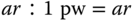 ph.
ph.
There are two common ways to attach an ![]() coordinate system to the image window, involving the location of the origin and the orientation of the
coordinate system to the image window, involving the location of the origin and the orientation of the ![]() and
and ![]() axes, as shown in Figure 2.2. The standard orientation used in mathematics to graph functions would place the origin at the lower left corner of the image with the
axes, as shown in Figure 2.2. The standard orientation used in mathematics to graph functions would place the origin at the lower left corner of the image with the ![]() ‐axis pointing upward. However, because traditionally images have been scanned from top to bottom, most image file formats store the image line‐by‐line, with the top line first, and line numbers increasing from top to bottom of the image. This makes the orientation shown in Figure 2.2(b) more convenient, with the origin in the upper left corner of the image and the
‐axis pointing upward. However, because traditionally images have been scanned from top to bottom, most image file formats store the image line‐by‐line, with the top line first, and line numbers increasing from top to bottom of the image. This makes the orientation shown in Figure 2.2(b) more convenient, with the origin in the upper left corner of the image and the ![]() ‐axis pointing downward. For this reason, we will generally use the orientation of Figure 2.2(b).
‐axis pointing downward. For this reason, we will generally use the orientation of Figure 2.2(b).
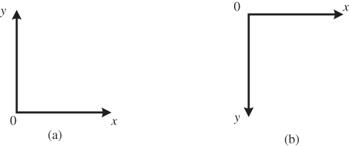
Figure 2.2 Orientation of  ‐axes. (a) Common bottom‐to‐top orientation in mathematics. (b) Scanning‐based top‐to‐bottom orientation.
2.2 Multidimensional Signals
A multiD signal can be considered to be a function from the domain, here ![]() , to the range. In this and the next few chapters, we consider only real and complex valued signals, which we call scalar signals. In later chapters, where we consider color signals, we will take the range to be a suitable vector space. In addition to naturally occurring continuous space‐time images, many analytically defined
, to the range. In this and the next few chapters, we consider only real and complex valued signals, which we call scalar signals. In later chapters, where we consider color signals, we will take the range to be a suitable vector space. In addition to naturally occurring continuous space‐time images, many analytically defined ![]() ‐dimensional functions are useful in image processing theory. A few of these are introduced here.
‐dimensional functions are useful in image processing theory. A few of these are introduced here.
2.2.1 Zero–One Functions
Let ![]() be a region in the
be a region in the ![]() ‐dimensional space,
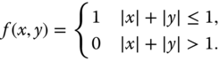
‐dimensional space, ![]() . We define the zero–one function
. We define the zero–one function ![]() as illustrated in Figure 2.3(a) by
as illustrated in Figure 2.3(a) by
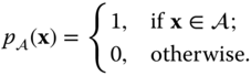
Sometimes, ![]() is called the indicator function of the region
is called the indicator function of the region ![]() . Different functions are obtained with different choices of the region
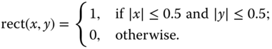
. Different functions are obtained with different choices of the region ![]() . Such functions arise frequently in modeling sensor elements or display elements (sub‐pixels). The most commonly used ones in image processing are the rect and the circ functions in two dimensions. Specifically, for a unit‐square region
. Such functions arise frequently in modeling sensor elements or display elements (sub‐pixels). The most commonly used ones in image processing are the rect and the circ functions in two dimensions. Specifically, for a unit‐square region ![]() we obtain (Figure 2.3(b))
we obtain (Figure 2.3(b))
For a circular region of unit radius we have (Figure 2.3(c))
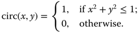
These definitions can be extended to the three‐dimensional case (where the region ![]() is a cube or a sphere) or to higher dimensions in a straightforward fashion, and the single notation
is a cube or a sphere) or to higher dimensions in a straightforward fashion, and the single notation ![]() or
or ![]() can be used to cover all cases. We will see later how these basic signals can be shifted, scaled, rotated or otherwise transformed to generate a much richer set of zero–one functions. Other zero–one functions that we will encounter correspond to various polygonal regions such as triangles, hexagons, octagons, etc.
can be used to cover all cases. We will see later how these basic signals can be shifted, scaled, rotated or otherwise transformed to generate a much richer set of zero–one functions. Other zero–one functions that we will encounter correspond to various polygonal regions such as triangles, hexagons, octagons, etc.
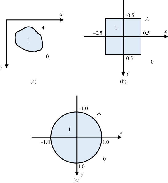
Figure 2.3 Zero–one functions. (a) General zero–one function. (b) Rect function. (c) Circ function.
2.2.2 Sinusoidal Signals
As in one‐dimensional signals and systems, real and complex‐exponential sinusoidal signals play an important role in the analysis of image processing systems. There are several reasons for this but a principal one is that if a complex‐exponential sinusoidal signal is applied as input to a linear shift‐invariant system (to be introduced shortly), the output is equal to the input multiplied by a complex scalar. A general, real two‐dimensional sinusoid with spatial frequency ![]() is given by
is given by
where ![]() and
and ![]() are spatial coordinates in ph (say),
are spatial coordinates in ph (say), ![]() and
and ![]() are fixed spatial frequencies in units of c/ph (cycles per picture height) and
are fixed spatial frequencies in units of c/ph (cycles per picture height) and ![]() is the phase. In general, for a given unit of spatial distance (e.g.,
is the phase. In general, for a given unit of spatial distance (e.g., ![]() m), spatial frequencies are measured in units of cycles per said unit (e.g., c/
m), spatial frequencies are measured in units of cycles per said unit (e.g., c/![]() m).
m).
Figure 2.4 illustrates a sinusoidal signal with horizontal frequency 1.5 c/ph and vertical frequency 2.5 c/ph in a square image window of size 1 ph by 1 ph. The actual signal displayed is ![]() , which has a range from 0 (black) to 1 (white). From this figure, we can identify a number of features of the spatial sinusoidal signal. The sinusoidal signal is periodic in both the horizontal and vertical directions, with horizontal period
, which has a range from 0 (black) to 1 (white). From this figure, we can identify a number of features of the spatial sinusoidal signal. The sinusoidal signal is periodic in both the horizontal and vertical directions, with horizontal period ![]() and vertical period
and vertical period ![]() . The signal
. The signal ![]() is constant if
is constant if ![]() is constant, i.e. along lines parallel to the line
is constant, i.e. along lines parallel to the line ![]() .
.
The one‐dimensional signal along any line through the origin is a sinusoidal function of distance along the line. The maximum frequency along any such line is ![]() , along the line
, along the line ![]() , as illustrated in Figure 2.4. The proof is left as an exercise.
, as illustrated in Figure 2.4. The proof is left as an exercise.
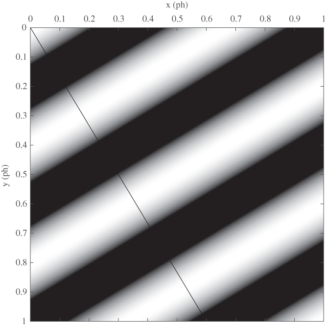
Figure 2.4 Sinusoidal signal with  = 1.5 c/ph and
  = 2.5 c/ph. The horizontal period is (2/3) ph and the vertical period is 0.4 ph. The frequency along the line
  is 2.9 c/ph, corresponding to a period of 0.34 ph.
As in one dimension, the complex exponential sinusoidal signals play an important role, e.g., in Fourier analysis. The complex exponential corresponding to the real sinusoid of Equation (2.4) is
where ![]() can be complex. In this book, we use j to denote
can be complex. In this book, we use j to denote ![]() . We often will adopt the vector notation
. We often will adopt the vector notation
where in the two‐dimensional case ![]() denotes
denotes ![]() as before,
as before, ![]() denotes
denotes ![]() and
and ![]() denotes
denotes ![]() . When using the column matrix notation, then
. When using the column matrix notation, then ![]() and we can write
and we can write ![]() . This is extended to any number of dimensions
. This is extended to any number of dimensions ![]() in a straightforward manner. Using Euler's formula, the complex exponential can be written in terms of real sinusoidal signals
in a straightforward manner. Using Euler's formula, the complex exponential can be written in terms of real sinusoidal signals
If ![]() is given as in Equation (2.6), then for any fixed
is given as in Equation (2.6), then for any fixed ![]() , we have
, we have
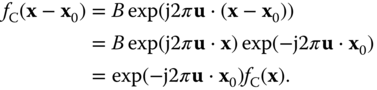
In other words, the shifted complex exponential is equal to the original complex exponential multiplied by the complex constant ![]() . This in turn leads to the key property of linear shift‐invariant systems mentioned earlier in this section. This will be analyzed in Section 2.5.5 but is mentioned here to motivate the importance of sinusoidal signals in multidimensional signal processing.
. This in turn leads to the key property of linear shift‐invariant systems mentioned earlier in this section. This will be analyzed in Section 2.5.5 but is mentioned here to motivate the importance of sinusoidal signals in multidimensional signal processing.
2.2.3 Real Exponential Functions
Real exponential signals also have wide applicability in multidimensional signal processing. First‐order exponential signals are given by
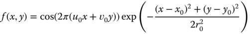
and second‐order, or Gaussian, signals by
Gaussian signals, similar in form to the Gaussian probability density, are widely used in image processing. Some illustrations can be seen later, in Figure 2.6. We define the standard versions of these signals as follows:
2.2.4 Zone Plate
A very useful two‐dimensional function that is often used as a test pattern in imaging systems is the zone plate, or Fresnel zone plate. The sinusoidal zone plate is based on the function
where ![]() is a parameter that sets the scale. Figure 2.5 illustrates the zone plate
is a parameter that sets the scale. Figure 2.5 illustrates the zone plate ![]() with
with ![]() ph. It is often convenient to consider the zone plate as the real part of the complex exponential function
ph. It is often convenient to consider the zone plate as the real part of the complex exponential function ![]() .
.
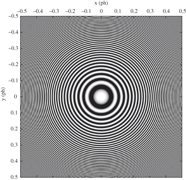
Figure 2.5 Illustration of a zone plate with parameter  ph. Local horizontal and vertical frequencies range from 0 to 125 c/ph.
Examining Figure 2.5, it can be seen that locally (say, within a small square window) the function is a sinusoidal signal with a horizontal frequency that increases with horizontal distance from the origin, and similarly a vertical frequency that increases with vertical distance from the origin. To make this concept of local frequency more precise, consider a conventional two‐dimensional sinusoidal signal
where ![]() . In this case we see that the horizontal and vertical frequencies are given by
. In this case we see that the horizontal and vertical frequencies are given by
We use these definitions to define the local frequency of a generalized sinusoidal signal ![]() . For the zone plate, we have
. For the zone plate, we have ![]() and so obtain
and so obtain
which confirms that local horizontal and vertical frequencies vary linearly with horizontal and vertical position respectively.
We define standard versions of the real and complex zone plates by
There is also a binary version of the zone plate that is widely used:
2.2.5 Singularities
As in one‐dimensional signals and systems, singularities play an important role in multiD signal and system analysis. These singularities are not functions in the conventional sense; they can be described as functionals and are often referred to as generalized functions, rigorously treated using distribution theory. However, following common practice, we will nevertheless sometimes refer to them as functions (e.g., delta functions). We present here some basic properties of singularities suitable for our purposes. More details can be found in Papoulis (1968) and Barrett and Myers (2004). A more rigorous but relatively accessible development is given in Richards and Youn (1990), and a careful development of signal processing using distribution theory can be found in Gasquet and Witomski (1999).
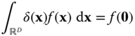
The 1D Dirac delta, denoted ![]() , is characterized by the property that
, is characterized by the property that
for any function ![]() that is continuous at
that is continuous at ![]() . In particular, taking
. In particular, taking ![]() , we have
, we have
The Dirac delta can be considered to be the limit of a sequence of narrow pulses of unit area, for example, ![]() or
or ![]() , as
, as ![]() .
.
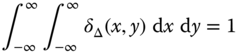
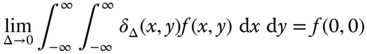
The 2D Dirac delta is defined in a similar fashion by the requirement
for any function ![]() that is continuous at
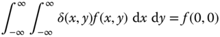
that is continuous at ![]() . Again, the 2D Dirac delta can be considered to be the limiting case of sequences of narrow 2D pulses of unit volume, e.g.,
. Again, the 2D Dirac delta can be considered to be the limiting case of sequences of narrow 2D pulses of unit volume, e.g.,
The 2D Dirac delta satisfies the scaling property
Other important properties of Dirac deltas will emerge as we investigate their role in multiD system analysis.
The Dirac delta can be extended to the multiD case in an obvious fashion, with the notation ![]() covering all cases. The conditions (2.20) and (2.22) are written
covering all cases. The conditions (2.20) and (2.22) are written
in the general case, where ![]() is understood to mean
is understood to mean ![]() ,
, ![]() or
or ![]() according to context. As a consequence of (2.23) in the general case,
according to context. As a consequence of (2.23) in the general case,
In addition to the point singularities defined above, we can have singularities on lines or curves in two or three dimensions, or on surfaces in three dimensions. See Papoulis (1968) for a discussion of singularities on a curve in two dimensions.
2.2.6 Separable and Isotropic Functions
A two‐dimensional function ![]() is said to be separable if it can be expressed as the product of one‐dimensional functions,
is said to be separable if it can be expressed as the product of one‐dimensional functions,
Several of the 2D functions we have seen are separable, including ![]() , the complex exponential
, the complex exponential ![]() , and the exponential functions. Also, the 2D Dirac delta
, and the exponential functions. Also, the 2D Dirac delta ![]() can be considered to be separable:
can be considered to be separable: ![]() . The extension to higher‐dimensional separable signals is evident,
. The extension to higher‐dimensional separable signals is evident,
Separability is a convenient way to generate multiD signals from 1D signals. Note that signals can also be separable in other variables than the standard orthogonal axes ![]() .
.
A 2D signal is said to be isotropic (circularly symmetric) if it is only a function of the distance ![]() from the origin,
from the origin,
Examples of isotropic signals that we have seen are ![]() , the Gaussian signal, and the zone plate. Again, the extension to multiD signals is evident:
, the Gaussian signal, and the zone plate. Again, the extension to multiD signals is evident: ![]() . We may also call such a signal rotation invariant, since it is invariant to a rotation of the domain
. We may also call such a signal rotation invariant, since it is invariant to a rotation of the domain ![]() about the origin.
about the origin.
2.3 Visualization of Two‐Dimensional Signals
It is easy to visualize a 1D signal ![]() by drawing its graph. If the graph is drawn to scale, we can derive numerical information by reading the graph, e.g.,
by drawing its graph. If the graph is drawn to scale, we can derive numerical information by reading the graph, e.g., ![]() . There are various ways that we can visualize a 2D signal. The three main visualization techniques are:
. There are various ways that we can visualize a 2D signal. The three main visualization techniques are:
- Intensity image: the signal range is transformed to the dynamic range of the display device and viewed as an image.
- Contour plot: this shows curves of equal value of the function to be displayed. The levels to be shown must be selected to get the most informative visualization, and they should be labeled if possible.
- Perspective plot: this shows a wireframe mesh of the surface as seen from a particular point of view. The density of the mesh and the point of view must be chosen for the best effect. Various ways of shading or coloring the perspective view can also be used.
Of course, method 1 is probably the most appropriate method to visualize a 2D signal that represents an image in the usual sense, but it may be useful in other cases as well. Contour and perspective plots are mainly useful for special 2D functions like the ones described in Section 2.2. Figure 2.6 illustrates the three visualization methods for a 2D Gaussian function. MATLAB provides all the necessary tools to generate such figures. See for example chapter 25 of Hanselman and Littlefield (2012) for a good description of how to generate such graphics in MATLAB.
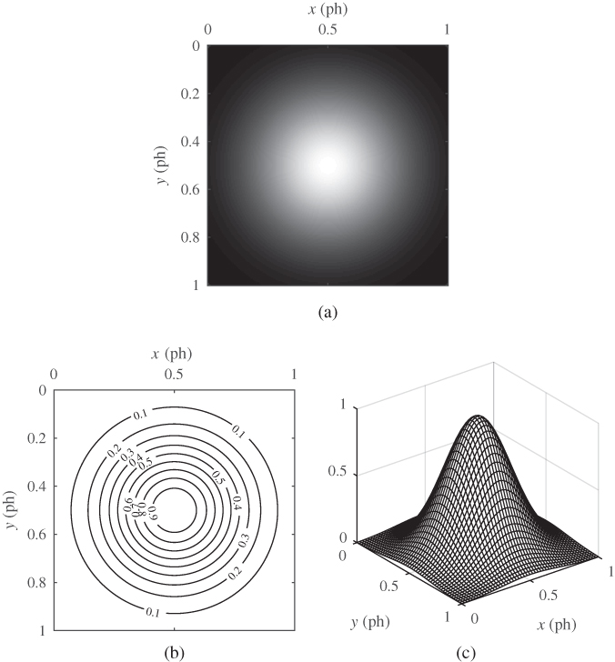
Figure 2.6 Visualization of a two‐dimensional Gaussian function centered at (0.5,0.5) and scaled with  ph. (a) Intensity plot. (b) Contour plot. (c) Perspective view.
2.4 Signal Spaces and Systems
A signal space ![]() is a collection of multiD signals defined on a specific domain
is a collection of multiD signals defined on a specific domain ![]() and satisfying certain well‐defined properties. For example, we can consider a space of all two‐dimensional signals
and satisfying certain well‐defined properties. For example, we can consider a space of all two‐dimensional signals ![]() defined for
defined for ![]() ,
, ![]() , or we can define a space of 2D signals defined on the spatial window
, or we can define a space of 2D signals defined on the spatial window ![]() of Figure 2.1. We can also impose additional constraints, such as boundedness, finite energy, or whatever constraints are appropriate for a given situation. An example of a specific signal space is
of Figure 2.1. We can also impose additional constraints, such as boundedness, finite energy, or whatever constraints are appropriate for a given situation. An example of a specific signal space is
As we will see later, we can also consider spaces of signals defined on discrete sets, corresponding to sampled images. We denote the fact that a given signal belongs to a signal space by ![]() . The object
. The object ![]() as a single entity is understood to encompass all the signal values
as a single entity is understood to encompass all the signal values ![]() as
as ![]() ranges over the specified domain of the signal space
ranges over the specified domain of the signal space ![]() .
.
A system ![]() transforms elements of a signal space
transforms elements of a signal space ![]() into elements of a second signal space
into elements of a second signal space ![]() according to some well‐defined rule. We write
according to some well‐defined rule. We write
where ![]() and
and ![]() . This equation can be read “the system
. This equation can be read “the system ![]() maps elements of
maps elements of ![]() into elements of
into elements of ![]() , where the element
, where the element ![]() is mapped to
is mapped to ![]() .” If
.” If ![]() , then we write
, then we write ![]() for the value of
for the value of ![]() at location
at location ![]() . In most cases,
. In most cases, ![]() and
and ![]() are the same, but sometimes they are different, e.g., for a system that samples a continuous‐space image to produce a discrete‐space image.
are the same, but sometimes they are different, e.g., for a system that samples a continuous‐space image to produce a discrete‐space image.
If we have two systems ![]() and
and ![]() , then we can apply
, then we can apply ![]() and
and ![]() successively to obtain a new system
successively to obtain a new system ![]() called the cascade of
called the cascade of ![]() and
and ![]() . As shown in Figure 2.7,
. As shown in Figure 2.7, ![]() and
and ![]() . Thus, we write
. Thus, we write ![]() .
.
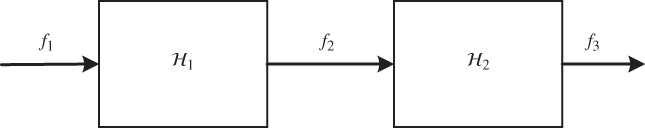
Figure 2.7 Cascade of two systems: 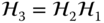 .
.
Alternatively, if the two systems have the same domain and range, ![]() and
and ![]() , they can be connected in parallel to give the new system
, they can be connected in parallel to give the new system ![]() defined by
defined by ![]() . In this case, we write
. In this case, we write ![]() .
.
2.5 Continuous‐Domain Linear Systems
Let ![]() be a system defined on a space
be a system defined on a space ![]() of continuous‐domain multiD signals with some domain
of continuous‐domain multiD signals with some domain ![]() . Many systems of practical interest satisfy the key property of linearity. This is convenient since linear systems are normally simpler to analyze than general nonlinear systems.
. Many systems of practical interest satisfy the key property of linearity. This is convenient since linear systems are normally simpler to analyze than general nonlinear systems.
2.5.1 Linear Systems
We first make the assumption that the signal space ![]() has the properties of a real or complex vector space. This ensures that elements of the signal space can be added together, and can be multiplied by a scalar constant, and that in each case the result also lies in the given signal space. This holds for most signal spaces of interest.
has the properties of a real or complex vector space. This ensures that elements of the signal space can be added together, and can be multiplied by a scalar constant, and that in each case the result also lies in the given signal space. This holds for most signal spaces of interest.
If ![]() and
and ![]() , then the sum
, then the sum ![]() is defined by
is defined by ![]() for all
for all ![]() . Similarly,
. Similarly, ![]() , the multiplication by a scalar, is defined by
, the multiplication by a scalar, is defined by ![]() for all
for all ![]() . Given these conditions, a system
. Given these conditions, a system ![]() is said to be linear if
is said to be linear if
for all ![]() ,
, ![]() and for all
and for all ![]() (or for all
(or for all ![]() for complex signal spaces). The definition of a linear system extends in an obvious fashion if
for complex signal spaces). The definition of a linear system extends in an obvious fashion if ![]() and
and ![]() in Equation (2.30) are different vector spaces. The most basic example of a linear system is
in Equation (2.30) are different vector spaces. The most basic example of a linear system is ![]() , which is easily seen to satisfy the definition. A system that does not satisfy the conditions of a linear system is said to be a nonlinear system. A simple and common example of a nonlinear system is given by
, which is easily seen to satisfy the definition. A system that does not satisfy the conditions of a linear system is said to be a nonlinear system. A simple and common example of a nonlinear system is given by ![]() .
.
Linear systems are of particular interest because if we know the response of the system to a number of basic signals ![]() , namely
, namely ![]() , then we can determine the response to any linear combination of the
, then we can determine the response to any linear combination of the ![]() :
:
As a simple example of a linear system, consider the shift (or translation) operator ![]() for some fixed shift vector
for some fixed shift vector ![]() . If
. If ![]() , then
, then ![]() . For this operation to be well defined, the domain of the signal space must be all of
. For this operation to be well defined, the domain of the signal space must be all of ![]() . In two dimensions, we would have
. In two dimensions, we would have ![]() , and
, and ![]() . It can easily be verified from the definitions that
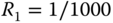
. It can easily be verified from the definitions that ![]() is a linear system. Figure 2.8 illustrates the shift operator with
is a linear system. Figure 2.8 illustrates the shift operator with ![]() .
.
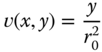
![2 Sets of xy planes with shaded box having 2 perpendicular lines depicting shift operator g = Τdf with d = [0.25,-0.25]T giving g(x, y) = f (x - 0.25, y + 0, 25).](http://images-20200215.ebookreading.net/2/1/1/9781119111740/9781119111740__multidimensional-signal-and__9781119111740__images__c02f008.jpg)
Figure 2.8 Shift operator  with
with  giving
  .
.
Another important class of linear systems consists of systems induced by an arbitrary nonsingular linear transformation of the domain ![]() for some
for some ![]() . Let
. Let ![]() be such a transformation, where
be such a transformation, where ![]() is a
is a ![]() nonsingular matrix. The induced system
nonsingular matrix. The induced system ![]() is defined by
is defined by
Again, it is easily verified from the definitions that ![]() is a linear system. We will mainly use this category of systems for scaling and rotating basic signals such as those of Section 2.2, but more general cases are widely used as well. If
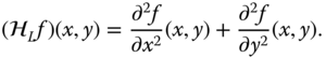
is a linear system. We will mainly use this category of systems for scaling and rotating basic signals such as those of Section 2.2, but more general cases are widely used as well. If ![]() is a diagonal matrix, the transformation
is a diagonal matrix, the transformation ![]() carries out a separate scaling along each of the axes, as illustrated in two dimensions in Figure 2.9(a). In this example,
carries out a separate scaling along each of the axes, as illustrated in two dimensions in Figure 2.9(a). In this example, ![]() , which has the effect of magnifying the image by a factor of two in each dimension. In general, if
, which has the effect of magnifying the image by a factor of two in each dimension. In general, if ![]() , the system
, the system ![]() will scale the image by a factor of
will scale the image by a factor of ![]() in the horizontal dimension and by
in the horizontal dimension and by ![]() in the vertical dimension.
in the vertical dimension.
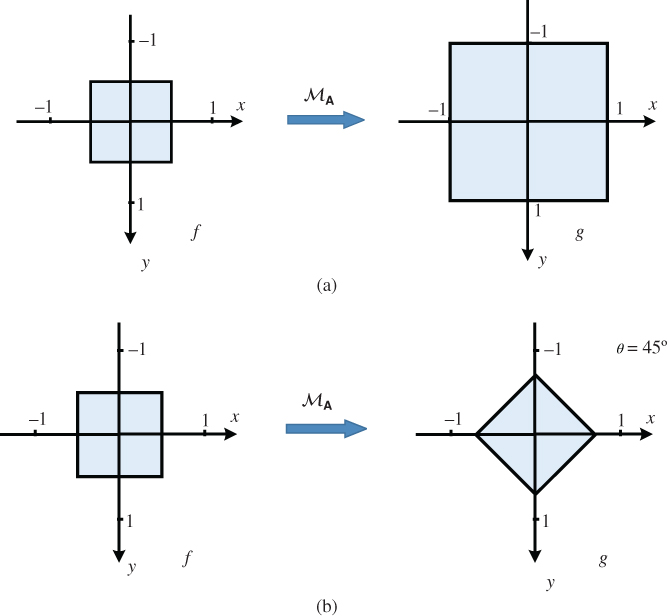
Figure 2.9 Transformations  . (a) Scale operator with
  . (b) Rotation operator with
  .
.
If ![]() is a two‐dimensional rotation matrix,
is a two‐dimensional rotation matrix,
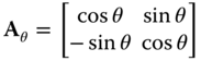
the transformation ![]() rotates the signal in the clockwise direction, as illustrated in Figure 2.9(b). The rotation of the domain
rotates the signal in the clockwise direction, as illustrated in Figure 2.9(b). The rotation of the domain ![]() is given by
is given by
where explicitly
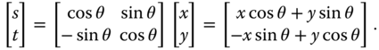
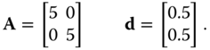
The rotation of the domain and the rotation of the signal are in opposite directions. Since this sometimes leads to confusion, we present a specific illustration. To demonstrate how ![]() acts on
acts on ![]() , consider the following four points, marked on Figure 2.10.
, consider the following four points, marked on Figure 2.10.
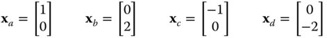
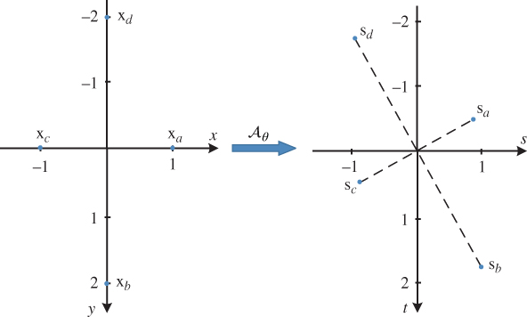
Figure 2.10 Illustration of the effect of a rotation operator with  on points in
  .
.
These points are mapped by ![]() to
to

These are marked on the right of Figure 2.10 for ![]() , where
, where ![]() and
and ![]() . We see that this transformation has rotated points in
. We see that this transformation has rotated points in ![]() counterclockwise by
counterclockwise by ![]() .
.
Now let us consider what happens when a two‐dimensional signal is mapped through the linear system given by Equation (2.34) for this transformation. Thus,
Thus, explicitly, ![]() . For example,
. For example,
This is illustrated in Figure 2.11, which shows the effect of applying this linear system to a diamond‐shaped zero‐one function. From the figure, we see that the linear system ![]() has rotated the two‐dimensional signal clockwise by
has rotated the two‐dimensional signal clockwise by ![]() , which is the opposite direction to that in which
, which is the opposite direction to that in which ![]() has rotated the points of
has rotated the points of ![]() .
.
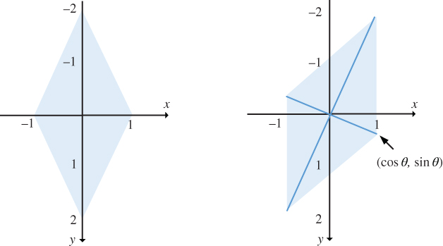
Figure 2.11 Illustration of the effect of a rotation operator with  on a zero‐one function with a diamond‐shaped region of support.
Another more general class of linear systems involves an affine transformation of the independent variables. One way to express this is
where ![]() is a nonsingular
is a nonsingular ![]() matrix. The affine transformation can be expressed as a cascade of the two preceding types of linear systems in two ways:
matrix. The affine transformation can be expressed as a cascade of the two preceding types of linear systems in two ways: ![]() . Generally the representation
. Generally the representation ![]() is more convenient. The signal is first rotated, scaled and perhaps sheared with respect to the origin, then centered at point
is more convenient. The signal is first rotated, scaled and perhaps sheared with respect to the origin, then centered at point ![]() . It can be shown that the cascade of any linear systems is also a linear system, and thus the system induced by an affine transformation of the domain is a linear system. As an example of an affine transformation, the Gaussian image of Figure 2.6 can be obtained from the unit variance, zero‐centered Gaussian
. It can be shown that the cascade of any linear systems is also a linear system, and thus the system induced by an affine transformation of the domain is a linear system. As an example of an affine transformation, the Gaussian image of Figure 2.6 can be obtained from the unit variance, zero‐centered Gaussian ![]() using the affine transformation with
using the affine transformation with
2.5.2 Linear Shift‐Invariant Systems
An important subclass of linear systems is the class of linear shift‐invariant (LSI) systems. In such a system, if the response to an input ![]() is
is ![]() , then if
, then if ![]() is shifted by any amount
is shifted by any amount ![]() , the resulting output is equal to
, the resulting output is equal to ![]() shifted by the same amount
shifted by the same amount ![]() . Using the above terminology, if
. Using the above terminology, if ![]() , then
, then ![]() for any
for any ![]() . For an LSI system
. For an LSI system ![]() ,
, ![]() for any
for any ![]() . We say that the two systems
. We say that the two systems ![]() and
and ![]() commute. The shift system
commute. The shift system ![]() is itself an LSI system, since
is itself an LSI system, since ![]() for any
for any ![]() . However, the general affine transformation system
. However, the general affine transformation system ![]() is not an LSI system if
is not an LSI system if ![]() , since
, since ![]() but
but ![]() .
.
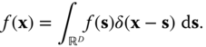
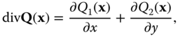
Another important class of LSI systems are those that involve partial derivatives of the input function with respect to the independent variables. As the simplest example, consider the 2D system ![]() defined by
defined by ![]() . Such systems are often connected in series or parallel, for example the system
. Such systems are often connected in series or parallel, for example the system ![]() , where the output is given by
, where the output is given by
This system is known as the Laplacian. This and other derivative‐based systems are further discussed in Section 2.7. Note that the series and cascade connection of LSI systems is also an LSI system. The proof is left as an exercise.
2.5.3 Response of a Linear System
The defining property of the Dirac delta function is given in Equation (2.24): ![]() . From this, we can derive the so‐called sifting property
. From this, we can derive the so‐called sifting property
This follows from

The sifting property (2.40) can be interpreted as the synthesis of the signal ![]() by the superposition of shifted Dirac delta functions
by the superposition of shifted Dirac delta functions ![]() with weights
with weights ![]() :
:
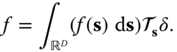
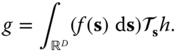
For a linear system ![]() , we can conclude that
, we can conclude that
where ![]() is the response of the system to a Dirac delta function located at position s. If we denote this impulse response
is the response of the system to a Dirac delta function located at position s. If we denote this impulse response ![]() , we obtain
, we obtain
It is important to recognize that while the above result is broadly valid and applies to essentially all cases of interest to us, the development is informal and there are many unstated assumptions. For example, the existence of ![]() (or more generally of
(or more generally of ![]() ) and the applicability of the linearity condition to an integral relation are assumed. The development can be treated more rigorously in several ways, such as assuming a specific signal space with a given metric, and assuming that the linear system is continuous. Then, an arbitrary signal can be approximated as a superposition of a finite number of pulse functions of the form
) and the applicability of the linearity condition to an integral relation are assumed. The development can be treated more rigorously in several ways, such as assuming a specific signal space with a given metric, and assuming that the linear system is continuous. Then, an arbitrary signal can be approximated as a superposition of a finite number of pulse functions of the form ![]() , and the output to this approximation determined. Taking the limit as
, and the output to this approximation determined. Taking the limit as ![]() and the extent tending to infinity yields the desired result. More details of this approach can be found in section 7.2 of Barrett and Myers (2004).
and the extent tending to infinity yields the desired result. More details of this approach can be found in section 7.2 of Barrett and Myers (2004).
2.5.4 Response of a Linear Shift‐Invariant System
Equation (2.43) describes the response of a general space‐variant linear system. Most optical systems are indeed space variant, with the response to an impulse in the corner of the image being different than the response to an impulse in the center of the image, for example. However, the design goal is usually to have a system that is as close to being shift invariant as possible. Thus, shift‐invariant systems are an important class. In this case,
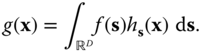
where ![]() is the response of the LSI system to an impulse at the origin, and so
is the response of the LSI system to an impulse at the origin, and so
Evaluating at position ![]() gives
gives
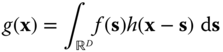
which is called the convolution integral, and is denoted
By a simple change of variables in the integral (2.46), we can show that ![]() , i.e. convolution is commutative.
, i.e. convolution is commutative.
2.5.5 Frequency Response of an LSI System
Suppose that the input to an LSI system is the complex sinusoidal function ![]() . According to Equation (2.46), the corresponding output is
. According to Equation (2.46), the corresponding output is
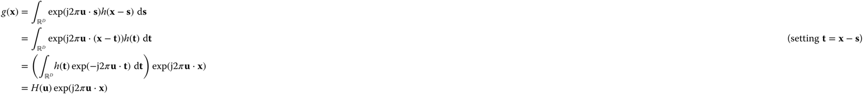
where ![]() is a complex scalar (assuming the integral converges). Thus, exactly as in one dimension, if the input to an LSI system is a complex sinusoidal signal with frequency vector
is a complex scalar (assuming the integral converges). Thus, exactly as in one dimension, if the input to an LSI system is a complex sinusoidal signal with frequency vector ![]() , then the output is that same complex sinusoidal signal multiplied by the complex scalar
, then the output is that same complex sinusoidal signal multiplied by the complex scalar ![]() . Taken as a function of the two or three‐dimensional frequency vector,
. Taken as a function of the two or three‐dimensional frequency vector, ![]() is referred to as the frequency response of the LSI system. According to this observation,
is referred to as the frequency response of the LSI system. According to this observation, ![]() is called an eigenfunction of the linear system
is called an eigenfunction of the linear system ![]() with corresponding eigenvalue
with corresponding eigenvalue ![]() .
.
Multiplication by ![]() amounts to multiplying the magnitude of
amounts to multiplying the magnitude of ![]() by
by ![]() and introducing a phase shift of
and introducing a phase shift of ![]() , i.e.
, i.e.
2.6 The Multidimensional Fourier Transform
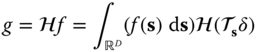
From Equation (2.48) we identify
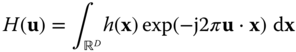
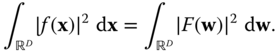
as the multiD extension of the continuous‐time Fourier transform. The multiD Fourier transform has properties that are completely analogous to the familiar properties of the 1D Fourier transform, as shown in Table 2.1. In particular, the inverse Fourier transform is given by
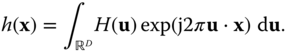
The reason for this will be given in Chapter 6. The Fourier transform can be applied to any signals in the signal space, not just the impulse response, as long as it converges. We denote that ![]() and
and ![]() form a multidimensional Fourier transform pair by
form a multidimensional Fourier transform pair by ![]() , where CDFT denotes continuous‐domain Fourier transform.
, where CDFT denotes continuous‐domain Fourier transform.
The property that makes the Fourier transform so valuable in linear system analysis is the convolution property (Property 2.4): the Fourier transform of ![]() is
is ![]() . Thus, if the input
. Thus, if the input ![]() to an LSI system with frequency response
to an LSI system with frequency response ![]() has Fourier transform
has Fourier transform ![]() , the output
, the output ![]() has Fourier transform
has Fourier transform ![]() .
.
Table 2.1 Multidimensional Fourier transform properties.
| (2.1) | ||
| (2.2) | ||
| (2.3) | ||
| (2.4) | ||
| (2.5) | ||
| (2.6) | ||
| (2.7) | ||
| (2.8) | ||
| (2.9) | ||
| (2.10) | ||
| (2.11) | ||
| (2.12) | ||
2.6.1 Fourier Transform Properties
The proofs of the properties in Table 2.1 are straightforward (aside from convergence issues) and similar to analogous proofs for the one‐dimensional Fourier transform, as given in many standard texts such as Bracewell (2000), Gray and Goodman (1995). They are presented briefly here. Again, the proofs are informal and assume that the relevant integrals converge, as would be the case for example if all the functions involved are absolutely integrable. Note that Property 2.6 relating to a linear transformation of the domain ![]() is a more complex generalization from the 1D case. In some proofs, we assume the validity of the inverse Fourier transform of Equation (2.51), although it has not been proved at this point.
is a more complex generalization from the 1D case. In some proofs, we assume the validity of the inverse Fourier transform of Equation (2.51), although it has not been proved at this point.
Note that using this property, commutativity and associativity of complex multiplication imply commutativity and associativity of convolution.
This property can be used to determine the effect of independent scaling of ![]() ‐ and
‐ and ![]() ‐axes, of rotation of the image, or of an affine transformation of the independent variable (along with the shifting property). For any rotation matrix
‐axes, of rotation of the image, or of an affine transformation of the independent variable (along with the shifting property). For any rotation matrix ![]() in
in ![]() dimensions,
dimensions, ![]() and
and ![]() (so
(so ![]() ), so that in this case
), so that in this case ![]() . Also, if
. Also, if ![]() , we get immediately that
, we get immediately that ![]() .
.
If ![]() , we obtain
, we obtain
2.6.2 Evaluation of Multidimensional Fourier Transforms
In general, the multiD Fourier transform is determined by direct evaluation of the defining integral (2.50) using standard methods of integral calculus. Simplifications are possible if the function ![]() is separable or isotropic, and of course maximum use should be made of the Fourier transform properties of Table 2.1. A few examples follow, and Table 2.2 provides a number of useful two‐dimensional Fourier transforms, and others are derived in the problems.
is separable or isotropic, and of course maximum use should be made of the Fourier transform properties of Table 2.1. A few examples follow, and Table 2.2 provides a number of useful two‐dimensional Fourier transforms, and others are derived in the problems.
Table 2.2 Two‐dimensional Fourier transform of selected functions.
 |
|
| 1 |
2.6.3 Two‐Dimensional Fourier Transform of Polygonal Zero–One Functions
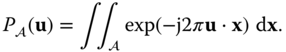
Polygonal zero–one functions are frequently encountered in the analysis of modern cameras and display devices, and their Fourier transform is required. For the rectangular region considered in Example 2.3, it is straightforward to compute the Fourier transform by direct evaluation of the integral. However, for other shapes, such as hexagons, octagons, chevrons, etc., direct computation of the Fourier transform is more involved and tedious. It is possible to convert the area integral in the direct definition of the Fourier transform to a line integral along the boundary of the region ![]() using the 2D version of Gauss's divergence theorem and thereby obtain a closed form expression for the Fourier transform in the case of polygonal regions.
using the 2D version of Gauss's divergence theorem and thereby obtain a closed form expression for the Fourier transform in the case of polygonal regions.
Let ![]() be a bounded, simply connected region in the plane and define
be a bounded, simply connected region in the plane and define ![]() as in Equation (2.1). Then, the Fourier transform is given by
as in Equation (2.1). Then, the Fourier transform is given by
Let ![]() be the boundary of
be the boundary of ![]() , assumed to be piecewise smooth, traversed in the clockwise direction. Then let
, assumed to be piecewise smooth, traversed in the clockwise direction. Then let ![]() be a vector field defined on
be a vector field defined on ![]() , assumed to be continuous with continuous first partial derivatives. The divergence theorem (see for example [(Kaplan, 1984, section 5.11)]) states that
, assumed to be continuous with continuous first partial derivatives. The divergence theorem (see for example [(Kaplan, 1984, section 5.11)]) states that
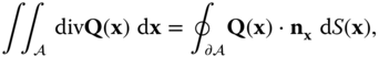
where
![]() is a unit vector normal to
is a unit vector normal to ![]() at
at ![]() and pointing outward, and
and pointing outward, and ![]() denotes arc length along
denotes arc length along ![]() at
at ![]() . This result can be applied to computing the Fourier transform in Equation (2.68) by choosing
. This result can be applied to computing the Fourier transform in Equation (2.68) by choosing
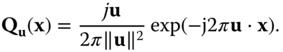
By applying the definition of divergence,
We then find that
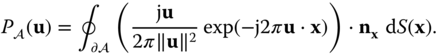
This result has been called the Abbe transform and was cited in the dissertation of Straubel in 1888 [Komrska (1982)]. As shown in Komrska (1982), the contour integral can easily be evaluated in closed form for a polygonal region as follows.
Assume that ![]() is a polygon with
is a polygon with ![]() sides, with vertices
sides, with vertices ![]() in the clockwise direction; for convenience, we denote
in the clockwise direction; for convenience, we denote ![]() . We define the following quantities that are easily determined once the vertices are specified:
. We define the following quantities that are easily determined once the vertices are specified:

where ![]() rotates counterclockwise by
rotates counterclockwise by ![]() . With these definitions, the Fourier transform expression given in Equation (2.73) can be written as a sum of the integrals over each of the polygon sides as follows.
. With these definitions, the Fourier transform expression given in Equation (2.73) can be written as a sum of the integrals over each of the polygon sides as follows.
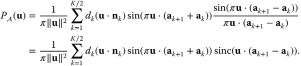
The integral can be easily evaluated to give the final result:
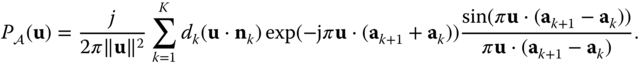
In many (but not all) cases of interest, the polygon is symmetric about the origin, i.e. ![]() . In this case, the number of vertices and sides is necessarily even, and the terms corresponding to the two opposite sides in Equation (2.79) can be combined to yield a real‐valued Fourier transform [Lu et al. (2009)].
. In this case, the number of vertices and sides is necessarily even, and the terms corresponding to the two opposite sides in Equation (2.79) can be combined to yield a real‐valued Fourier transform [Lu et al. (2009)].
This result has been extended to zero–one functions in more than two dimensions where the region of support is a polytope [Brandolini et al. (1997)], and applications in multiD signal processing have been described in Lu et al. (2009).
It is very straightforward to apply this result to determine the Fourier transform of a rect function, and this is left as an exercise. The following shows the application to a regular hexagon with unit side.
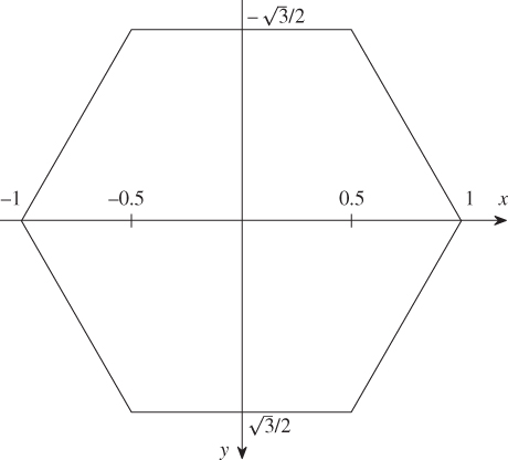
Figure 2.12 Regular hexagon with unit side.
2.6.4 Fourier Transform of a Translating Still Image
Assume that a still image ![]() is moving with a uniform velocity
is moving with a uniform velocity ![]() to produce the time‐varying image
to produce the time‐varying image ![]() . We wish to relate the 3D Fourier transform of
. We wish to relate the 3D Fourier transform of ![]() to the 2D Fourier transform of
to the 2D Fourier transform of ![]() .
.
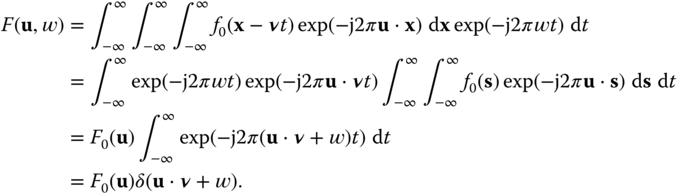
Thus, the 3D Fourier transform is concentrated on the plane ![]() . This leads us to conclude that the 3D Fourier transform of a typical time‐varying image is not uniformly spread out in 3D frequency space, but will be largely concentrated near planes representing the dominant motions in the scene.
. This leads us to conclude that the 3D Fourier transform of a typical time‐varying image is not uniformly spread out in 3D frequency space, but will be largely concentrated near planes representing the dominant motions in the scene.
2.7 Further Properties of Differentiation and Related Systems
Image derivatives are frequently used in the image processing literature. Although generally applied to discrete‐domain images, where derivatives are not defined, they usually presuppose an underlying continuous‐domain image where derivatives are defined. Thus we introduce here several additional continuous‐domain LSI systems based on derivatives, beyond the gradient already seen in Property 2.7.
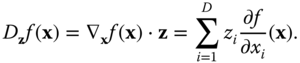
2.7.1 Directional Derivative
Let ![]() be a unit vector in
be a unit vector in ![]() . The directional derivative is a scalar function giving the rate of change of
. The directional derivative is a scalar function giving the rate of change of ![]() in the direction
in the direction ![]() . This can be denoted
. This can be denoted
We assume ![]() is continuous at
is continuous at ![]() . From standard multivariable calculus, we know that
. From standard multivariable calculus, we know that
The magnitude of the directional derivative ![]() is maximum when the unit vector
is maximum when the unit vector ![]() is collinear with the gradient
is collinear with the gradient ![]() , and it is zero when
, and it is zero when ![]() is orthogonal to the gradient. As a result, the gradient is often used to quantify the local directionality of
is orthogonal to the gradient. As a result, the gradient is often used to quantify the local directionality of ![]() . Although this result is quite evident from standard vector analysis, the following matrix proof leads to many interesting generalizations. We can express the magnitude squared of the directional derivative as
. Although this result is quite evident from standard vector analysis, the following matrix proof leads to many interesting generalizations. We can express the magnitude squared of the directional derivative as
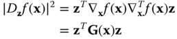
where ![]() . This is maximized when
. This is maximized when ![]() is the normalized eigenvector corresponding to the maximum eigenvalue of
is the normalized eigenvector corresponding to the maximum eigenvalue of ![]() . Since
. Since ![]() has rank one and thus the null space has dimension
has rank one and thus the null space has dimension ![]() , it follows that
, it follows that ![]() eigenvalues are zero. The eigenvector corresponding to the one non‐zero eigenvalue is
eigenvalues are zero. The eigenvector corresponding to the one non‐zero eigenvalue is ![]() , since
, since
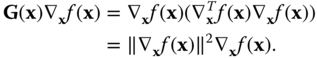
Then, the maximum value of ![]() is
is ![]() , which occurs for
, which occurs for ![]() , as stated previously. The entity
, as stated previously. The entity ![]() is usually referred to as the structure tensor, and this is a quantity that has many generalizations.
is usually referred to as the structure tensor, and this is a quantity that has many generalizations.
The Fourier transform of ![]() is then given by
is then given by ![]() . Thus, the directional derivative is a linear shift‐invariant system with frequency response
. Thus, the directional derivative is a linear shift‐invariant system with frequency response ![]() .
.
2.7.2 Laplacian
The Laplacian is a scalar system involving second order derivatives, typically denoted ![]() :
:
If ![]() , the Fourier transform of the output of the Laplacian is given by
, the Fourier transform of the output of the Laplacian is given by
Thus, the Laplacian is an LSI system, with frequency response ![]() , which is isotropic.
, which is isotropic.
2.7.3 Filtered Derivative Systems
The derivative systems presented so far have frequency responses that increase in magnitude with ![]() . This makes them very sensitive to high‐frequency noise, and they are regularly coupled with low‐pass filters. For example, the gradient and Laplacian are frequently preceded with Gaussian filters to smooth the high frequencies before applying the gradient, Laplacian or higher‐order derivative operator. When using these to analyze the image, the Gaussian filter can also serve to set the scale at which the analysis takes place.
. This makes them very sensitive to high‐frequency noise, and they are regularly coupled with low‐pass filters. For example, the gradient and Laplacian are frequently preceded with Gaussian filters to smooth the high frequencies before applying the gradient, Laplacian or higher‐order derivative operator. When using these to analyze the image, the Gaussian filter can also serve to set the scale at which the analysis takes place.
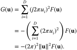
As an example, consider the Laplacian that is an isotropic scalar system. It is usually coupled with an isotropic Gaussian low‐pass filter with impulse response and frequency response
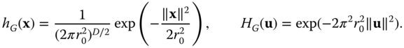
Thus, the filtered Laplacian has frequency response
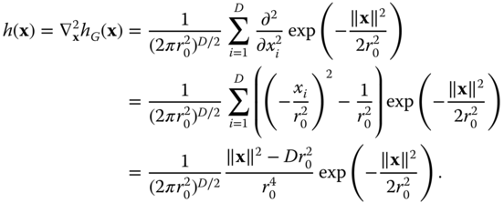
Using the associative property of LSI systems, the impulse response of the filtered Laplacian is given by the Laplacian of the Gaussian impulse response (so it is called a Laplacian of Gaussian or LoG filter):
The filtered Laplacian is most frequently used in two dimensions, where the frequency response and the impulse response can be written
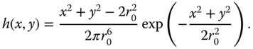
In general, the absolute magnitude of ![]() is not significant, and it can be scaled to any convenient value. The frequency response is circularly symmetric with value 0 at the origin and for large frequency, and a peak amplitude at the radial frequency
is not significant, and it can be scaled to any convenient value. The frequency response is circularly symmetric with value 0 at the origin and for large frequency, and a peak amplitude at the radial frequency ![]() . Figure 2.13 depicts the impulse response and magnitude frequency response of a LoG filter with
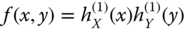
. Figure 2.13 depicts the impulse response and magnitude frequency response of a LoG filter with ![]() ph. The filter is scaled so that the maximum magnitude frequency response is 1.0, which occurs at radial frequency 90 c/ph. Figure 2.14 shows a simulation of the filtering of the ‘Barbara’ image with this LoG filter. Since the mean output level of the filtered image is 0, a value of 0.5 on a scale of 0 to 1 is added to the image for the purpose of display.
ph. The filter is scaled so that the maximum magnitude frequency response is 1.0, which occurs at radial frequency 90 c/ph. Figure 2.14 shows a simulation of the filtering of the ‘Barbara’ image with this LoG filter. Since the mean output level of the filtered image is 0, a value of 0.5 on a scale of 0 to 1 is added to the image for the purpose of display.
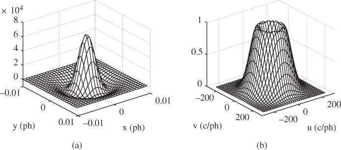
Figure 2.13 Laplacian of Gaussian filter with  . (a) Negative of impulse response. (b) Magnitude of frequency response.

Figure 2.14 Laplacian of Gaussian filter with  applied to ‘Barbara’ image.
Problems
- 1
Consider a two‐dimensional sinusoidal signal
 where
where  and
and  are in ph and
  and
and  are in c/ph. Form the one‐dimensional signal
  by tracing
  along the line
  , where
  is some real constant, as a function of distance along the line,
  .
.
- Show that
 is a sinusoidal signal
 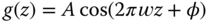 and determine the spatial frequency
  in c/ph, as a function of
  ,
,  and
and  .
. - Explain what happens when
 and when
  .
. - Show that the spatial frequency
 is greatest along the line
 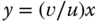 , if
, if  . What is the value of this maximum spatial frequency? What happens if
  ?
?
- Show that
- 2 Show that for each of the following functions
 ,
,
and
for any function
 that is continuous at
  .
.
 .
.
- 3 Show that
where
 .
. - 4
Prove that the following systems are linear systems.
- The shift system
 for any shift
  .
. - The system induced by a nonsingular transformation of the domain,
 , where
  is any nonsingular
  matrix.
 - The cascade of two linear systems
 and
and  . Thus, the system induced by an affine transformation of the domain is a linear system.
 - The parallel combination of two linear systems with the same domain and range,
 .
. - The partial derivative systems
 and
and  defined in Section 2.5.2.
- The shift system
- 5
Prove that the following systems are linear shift‐invariant systems.
- The shift system
 for any shift
  .
. - The cascade of two LSI systems
 and
and  .
. - The parallel combination of two LSI systems with the same domain and range,
 .
. - The partial derivative systems
 and
and  defined in Section 2.5.2.
- The shift system
- 6
Let
 and
and  , where
  and
and  are in ph.
- Sketch the region of support of
 and
and  in the
  ‐plane (i.e., the area where these two signals are nonzero).
 - Compute the two‐dimensional convolution
 from the definition using integration in the spatial domain.
 - Suppose that
 is the input to a 2D system, and the output of this system is computed as in (b). What can we say about this system?
 - Determine the continuous‐space Fourier transforms
 ,
,  and
and  of the above three signals. Make liberal use of Fourier transform properties. What are the units of
  and
and  ?
? - Continuing with question (c), what is the interpretation of
 ?
?
- Sketch the region of support of
- 7
Determine the response of an LSI system with impulse response
 to a real sinusoidal signal
  where
where  and
and  .
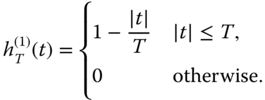
. - 8 A 2D continuous‐space linear shift‐invariant system has impulse response
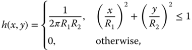
where
 ph and
 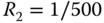 ph.
ph.- Sketch the region of support of the impulse response in the
 ‐plane, following the conventions used for the labelling of axes. Express
  in terms of the circ function.
 - Find the frequency response
 of this system, where
  and
and  are in c/ph.
 - The image
 is filtered with this system to produce the output
 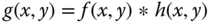 . Determine the Fourier transform of the output,
  .
.
- Sketch the region of support of the impulse response in the
- 9
Compute the two‐dimensional continuous‐space Fourier transform of the following signals:
- The separable signal
 where
where
- A Gaussian function
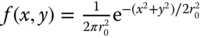 . (i) Obtain the result from the entry in Table 2.2 (with
  ). (ii) Prove the result in Table 2.2.
 - A real zone plate,
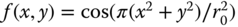 . (Hint: Find the Fourier transform of the complex zone plate
 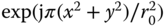 and use linearity. You can use
  .)
.) - Diamond‐shaped pulse
(Hint: obtain this function from a rect function using a rotation transformation.)
- Gabor function
- The 2D zero–one function
 where
where  is an elliptical region, with semi‐minor axis
  and semi‐major axis
  , oriented at
  as shown in Figure 2.15
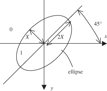
Figure 2.15 Elliptical region of support of a 2D zero–one function.
- The separable signal
- 10 Derive the expression for the Fourier transform of a zero–one function on a polygon symmetric about the origin, as given in Equation (2.80).
- 11 Use the expression in Equation (2.80) to compute the Fourier transform of the rect function.
- 12
Use the expression in Equation (2.80) to compute the Fourier transform of a zero‐one function with a region
 that is a regular hexagon of unit area, with vertices on the
  ‐axis.
 - 13
Use the expression in Equation (2.80) to compute the Fourier transform of a zero–one function with a region
 that is a regular octagon of unit area, with two sides parallel to the
  ‐axis.
 - 14 Consider a continuous‐domain Laplacian of Gaussian (LoG) filter with impulse response
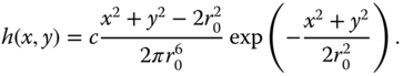
- Show that the magnitude frequency response has a peak at radial frequency
- What is the value of
 such that the peak magnitude frequency response is 1.0, i.e.,
- Compute the values found in (a) and (b) when
 ph.
ph.
- Show that the magnitude frequency response has a peak at radial frequency
- 15
Find the
 ‐dimensional Fourier transform of the following functions: