
Chapter 4
Analyzing Resources
Edward A. Pohl
Department of Industrial Engineering, University of Arkansas, Fayetteville, AR, USA
Simon R. Goerger
Institute for Systems Engineering Research, Information Technology Laboratory (ITL), U.S. Army Engineer Research and Development Center (ERDC), Vicksburg, MS, USA
Kirk Michealson
Tackle Solutions, LLC, Chesapeake, VA, USA
Decision-making . . . is the irrevocable commitment of resources today for results tomorrow.
(George K. Chacko (Chacko, 1990, p. 5))
For which of you, intending to build a tower, does not first sit down and estimate the cost, to see whether he has enough to complete it? – Unknown
4.1 Introduction
A fundamental fact of decision-making includes the commitment of resources. Resources are essential assets committed to perform a trade-off analysis and to execute the subsequent decision. They come in many forms and include the following: money, facilities, time, people, and cognitive effort. Resources required for possible resolution of an issue are included in the resource space (Figure 4.1). To better understand the cost of each alternative, it is necessary to identify the required set(s) of resources, define the resource space, and determine which resources will be committed for each alternative.
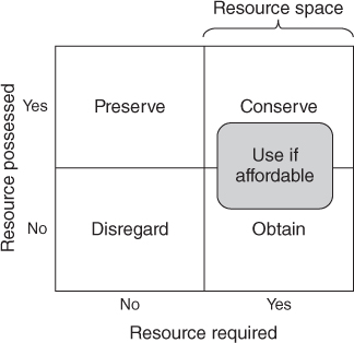
Figure 4.1 Resource space
This chapter discusses the resource categories that comprise a resource space, techniques to determine the cost of resources for proposed alternatives, and means for assessing the affordability of the alternatives. Using these techniques in a logical and repeatable manner helps to understand the resource impacts of trade-off analysis alternatives.
4.2 Resources
A resource is an asset accessible for use in producing the benefits of a decision. In identifying resources, it is useful to have a framework to ensure that you more fully capture the type and quantity of resources. The type and amount of resources available to support a decision are defined as the trade-off analysis resource space. This section discusses three components of the resource space: people, facilities, and costs. Figure 4.2 illustrates the three components. People and facilities can also be considered as “cost.” In this section, they are broken down as separate resources to facilitate their description.
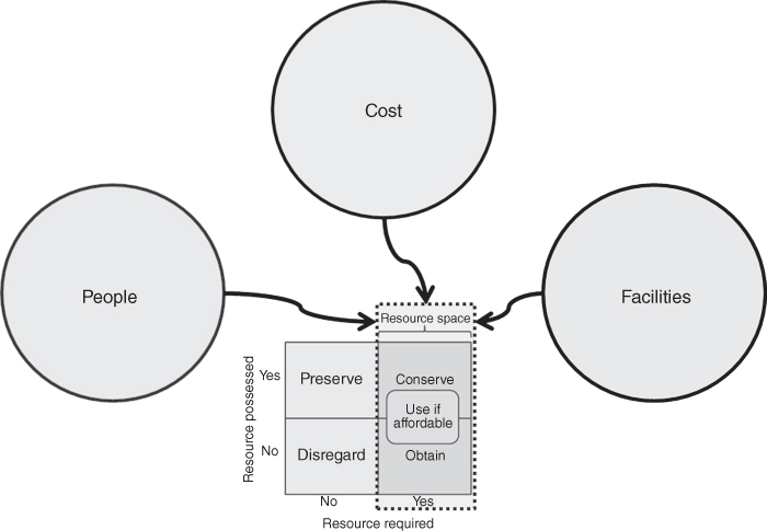
Figure 4.2 The three components of the resource space
4.2.1 People
People and the skills they possess are essential to effectively implement a decision. They provide the means to leverage assets and accomplish the vision and goals of the decision. Therefore, it is crucial to identify what skills are on hand, the skills each solution requires to be successfully implemented, and what skills will need to be obtained via external organizations. Personnel skills can be binned into generalizable capabilities and further broken down into subspecialties. General skill bins are hard skills and soft skills. Soft skills are interpersonal and tend be more intrinsic than hard skills, which are more learned knowledge and quantifiable abilities. Both are required for success in a job. Figure 4.3 provides an example of hard and soft skills for people resources.
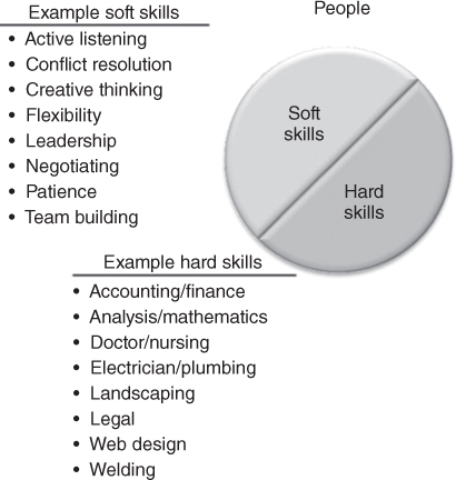
Figure 4.3 Example of skills for people resources
The soft skills bin consists of numerous interpersonal skills. Table 4.1 lists some examples of these skills.
Table 4.1 Example Soft Skills
| Active listening | Collaboration | Conflict management |
| Conflict resolution | Consulting | Counseling |
| Creative thinking | Customer service | Diplomacy |
| Flexibility | Instructing | Interviewing |
| Leadership | Mediating | Mentoring |
| Negotiating | Networking | Nonverbal communication |
| Patience | Persuasion | Problem solving |
| Team building | Teamwork | Verbal communication |
Table 4.2 is an example list of hard skills one should consider when determining the team capabilities and skills required to execute a decision. These skills can be physical or analytical in nature, but require education or training to attain or maintain.
Table 4.2 Example Hard Skills
| Accounting | Analysis | Computer programming |
| Construction | Doctor/nursing | Electrician |
| Finance | Flying | Heavy equipment operator |
| Landscaping | Law | Machining |
| Mathematics | Plumbing | Typing |
| Web design | Welding | Writing |
The skills people possess allow them to perform various roles in the execution of a decision such as executive, management, customer service, communication, operation, maintenance, and logistics. These roles often require a combination of soft and hard skills. Based on changes that occur during the execution of a decision, managers often require the use of soft skills such as active listening, critical thinking, flexibility, problem solving, and conflict resolution as well hard skills such as technical knowledge of the area of interest to identify issues and solutions that will help execute a decision. Table 4.3 is an example list of hard and soft skills that a manager may need to facilitate the execution of a decision. Executive, management, customer service, and communication roles tend to include more soft skills while those personnel performing the roles of operations, maintenance, and logistics tend to have more hard skills.
Table 4.3 Example Set of Hard and Soft Skills for Management
| (S) Adaptability | (H) Administrative | (H) Analytical ability |
| (S) Assertiveness | (H) Budget management | (H) Business management |
| (S) Collaboration | (S) Conflict management | (S) Conflict resolution |
| (S) Coordination | (S) Critical thinking | (S) Decision-making |
| (S) Delegation | (S) Empowerment | (H) Financial management |
| (S) Flexibility | (S) Focus | (S) Goal setting |
| (S) Innovation | (S) Interpersonal | (S) Leadership |
| (H) Legal | (S) Listening | (S) Nonverbal communication |
| (S) Obstacle removal | (S) Organizing | (H) Planning |
| (S) Problem-solving | (H) Process management | (H) Product management |
| (S) Professionalism | (H) Project management | (H) Scheduling |
| (S) Staffing | (S) Team building | (S) Team manager |
| (S) Team player | (H) Technical knowledge | (H) Time management |
| (S) Verbal communication | (S) Vision | (S) Writing |
(H) – Hard skills; (S) – Soft skills.
Table 4.4 is an example set of functions for the roles present in an organization. Based on these roles and the personnel in these roles, an inventory of hard and soft skills can be conducted.
Table 4.4 Example Set of Roles and Functions for People Resources
| Role | Example Functions |
| Executive |
|
| Management |
|
| Budget |
|
| Customer service |
|
| Communication |
|
| Operations |
|
| Maintenance |
|
| Logistics |
|
Inventorying the skills and quantity of the skills possessed by an organization is half the question. For each course of action, it is imperative to assess the skills and quantify requirements. This information will be used to help assess what additional people skills will be required to execute each option.
4.2.2 Facilities
Facility (or capital asset) resources are durable assets used in the production of products and/or services. Examples include tools, vehicles, roads, ships, plans, waterways, airports, machines, office space, communications equipment and infrastructure, power grid, and factories. These can be binned as infrastructure or equipment. Figure 4.4 is an illustration of the types of facility resources.
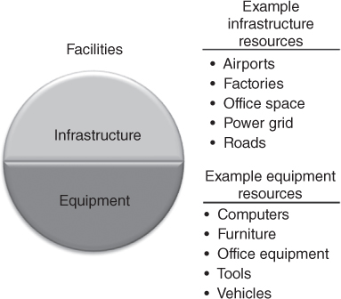
Figure 4.4 Example of types of facility resources
Table 4.5 provides an example list of these facility categories by bin. As with personnel, management must ascertain the types, numbers, and capacity of each facility asset they control.
Table 4.5 Facility Examples
| Infrastructure | Equipment |
| Airports | Cars |
| Communications infrastructure | Communications equipment |
| Factories | Computers |
| Office space | Furniture |
| Power grid | Machines |
| Power plants | Office equipment |
| Roads | Planes |
| Schools | Robots |
| Stores | Ships |
| Warehouses | Tools |
| Waterways | Trucks |
4.2.3 Costs
Most people think of currency when they hear the term cost (e.g. Dollars, Euros, Pounds, Renminbi, Rubles, and Bitcoin). However, cost refers to any term used to represent resources of an organization. These include people (labor), facilities, and hours. Cost is an essential factor of a trade-off analysis as it can help to place resources, products, and services into a unifying quantitative measure that is more easily understood by analysts and decision makers. (Parnell et al., 2011, pp. 143–144)
There are several types of costs whether you are enhancing an existing system or developing a new one. The types of costs and their magnitude differ based on the type of system and the life cycle phase of the system. The Department of Defense defines five phases for its Acquisition Life Cycle and subsequent cost modeling. These five phases are as follows: (i) Material Solution Analysis (MSA), (ii) Technology Maturation and Risk Reduction (TMRR), (iii) Engineering and Manufacturing Development (EMD), (iv) Production and Deployment (P&D), and (v) Operations and Support (O&S). Each phase is preceded by a milestone or decision point. During the phases of the Acquisition Life Cycle, a system goes through research, development, test, and evaluation (RDT&E); production; fielding or deployment; sustainment; and disposal (Acquisition Life Cycle, 2015). When considering the entire life cycle of a system, we need to consider five cost classifications to identify the sources and effects of these sources on a system's life cycle: development, construction, acquire, O&S, and system retirement.1
Stewart et al. divided cost into four separate classes, which occur across the phases of a program or system life cycle: (i) acquisition, (ii) fixed and variable, (iii) recurring and nonrecurring, and (iv) direct and indirect (Stewart et al., 1995). These are not four elements of the same analysis, but instead four separate ways to classify costs. The remainder of this section defines these classes of cost. Section 4.3 discusses the use of these classes for calculating and using these costs in assessing the resource space.
4.2.3.1 Acquisition (Operate, Sustain, and Dispose) Costs
These are the total costs associated with the concept, design, development, production, or deployment of system or process (e.g., buildings, bridges, communications systems, vehicles, etc.). It does not include the cost to operate, sustain, or dispose of a product or process.
4.2.3.2 Fixed and Variable Costs
An organization incurs fixed or sunk cost, no matter the phase of the system life cycle a product is in or the quantity of products produced. These independent costs of the program may include the cost of maintaining a research team, long-term rental cost for facilities, depreciation of equipment value, taxes (local, state, and federal), insurance for permanent assets, and site security. Variable costs vary based on the number and types produced or operated. These costs can easily be associated with each unit produced. Examples of variable costs include direct labor, material, and energy for the production of a product.
4.2.3.3 Recurring and Nonrecurring Costs
Similarly to variable costs, recurring costs are associated with each unit produced or each time the process is executed. Unlike variable costs, recurring costs may not vary with the number or type of products produced. For example, the annual property taxes are recurring and fixed costs. Nonrecurring costs are those incurred only once in the life cycle or expected to be incurred only once in a life cycle. An example of nonrecurring costs include the resources required for initial design and testing as these tasks occur only once for each product.
4.2.3.4 Direct and Indirect Costs
Direct costs are associated with a specific system, product, process, or service. These costs are often subdivided into direct labor, direct material, or direct expense costs. These cost subdivisions are similar to examples of variable costs. Labor costs associated with a specific product are considered direct labor cost, while fixed labor costs such as plant security and janitorial services are often considered indirect costs. Thus, indirect costs are costs that cannot easily be assigned to a specific product or process. Overhead costs such as executive leadership, human resources, accounting, annual training, and grounds maintenance are traditionally categorized as indirect costs. An example of an indirect, variable, recurring cost would be the energy used for the guard shack and lights on the overflow yard/warehouse used to stage excess products produced for the holiday surge in demand. Cost estimates routinely do a better job of identifying direct costs, but often fall short with identifying accurate indirect costs. To obtain more accurate indirect cost estimates, a life cycle cost (LCC) technique called activity-based costing may be used. This technique subdivides indirect costs by functional activities executed during the system life cycle (Canada et al., 2005). The costs associated with each activity are further defined by defined cost drivers to help identify which costs could be appreciated against a specific product or service.
Based on these classes of cost, any single cost could be categorized into several classes (Figure 4.5). For example, management cost for a multiyear product line could be classified as acqusiton, fixed, reccuring, indirect costs as it is performed across all phases of the life cycle as part of the organization's structure and processes. Management costs could also be variable depending on how many shifts are needed to produce a product. The management costs could be nonrecurring and direct if a part-time manager was hired to temporaraily run the night shift.
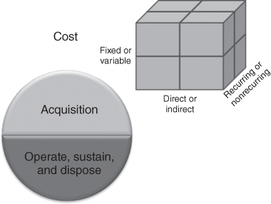
Figure 4.5 Cost resource by class
4.2.4 Resource Space
Once resources have been identified, one must determine if they reside within the nexus of resources for the organization. This nexus is the preliminary resource space and consists of the list of the resources, the required quantities, the duration and time of their use, and the cost of their use. The products from this effort are used for resource analyses. Figure 4.6 is an example resource framework to facilitate the identification and cost classification of resources in a preliminary resource space.
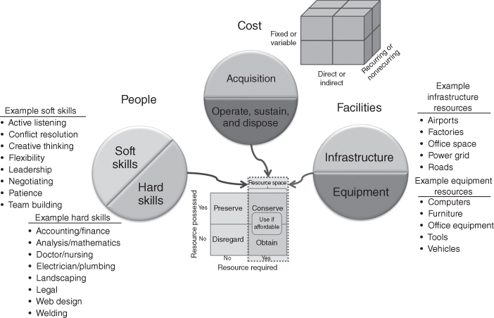
Figure 4.6 Example resource framework
4.3 Cost Analysis
A system is defined as “an integrated set of elements that accomplishes a defined objective. System elements include products (hardware, software, firmware), processes, people, information, techniques, facilities, services, and other support elements” (International Committee for Systems Engineering (INCOSE), 2015). All systems have a specific life cycle. There are many system life cycle models in the literature. For example, a common system life cycle in the system engineering literature consists of seven stages: (Parnell et al., 2011, pp. 7–9) conceptualization, design, development, production, deployment, operation, and retirement of the system. Throughout each of these stages, various levels of LCCs occur and trade-offs are made that impact the future costs of development, production, support, and disposal costs of the system.
Capturing system LCCs is necessary to make reasonable trade-offs during design, development, production, and operations. A LCC model is used by a systems engineering team in a trade-off analysis to estimate whether new alternatives or proposed system modifications meet a specific set of functional requirements at an affordable total cost over the duration of its anticipated life. When successfully performed, life cycle costing is an effective trade-off analysis tool that can be used throughout the life cycle of a system. The Society of Cost Estimating and Analysis (Glossary, 2015) defines a LCC estimate in the following way.
The concept map for life cycle costing is provided by Parnell et al. (2011, p. 138), as shown in Figure 4.7. This figure provides a pictorial illustration of the key elements that contribute to develop a comprehensive life cycle assessment. The LCC assessment centers around the development of a system's cost estimate, which in conjunction with a project schedule is used to manage a system's design, development, production, as well as operation, and disposal. System design and operational concepts drive the key cost parameters, which in turn identify the data required for developing a system cost estimate. As part of a systems engineering and trade-off analysis team, cost analysts and engineers rely on historical data, subject matter experts (SME), system schedules, and budget quantities to provide data to use for life cycle costing techniques. In addition, risk plays a key role in LCC estimates. Risk affects the key cost parameters that drive the system cost estimate and is largely driven by the stage of development the system is in as well as the complexity and technology being utilized in the system design.
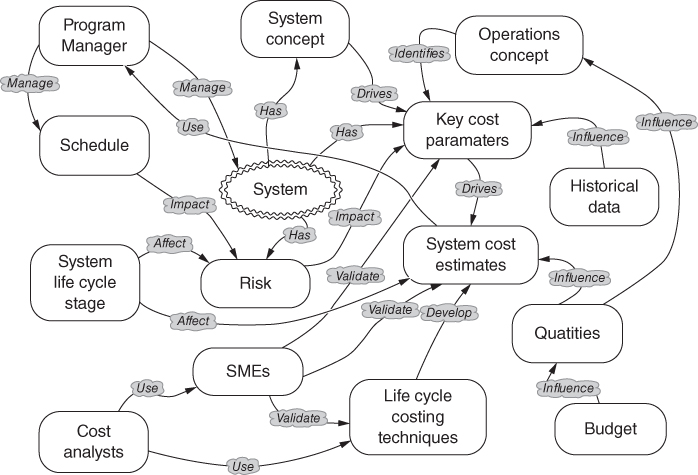
Figure 4.7 Life cycle costing concept map (Source: Parnell et al. 2011. Reproduced with permission of John Wiley & Sons)
Cost estimation is a critical activity and key to the perceived success of complex public and private projects. Cost estimates should be developed and refined for all stages of a system life cycle. For example, cost estimates are used to develop a budget for the development of a new system or technology, to prepare a bid on a complex system proposal, to negotiate a purchase price for a system of systems, and to provide a baseline from which to track and manage actual costs and make trade-offs during all stages of development and operations of large-scale complex systems.
Selection of the most appropriate LCC technique depends largely on the quantity and type of data available as well as the perceived system risks. Data can be system specification and/or from historic cost data or models. As each stage of the life cycle progresses, additional information concerning system design and system performance becomes available, and some uncertainty is resolved while new uncertainties may be introduced. Therefore, selecting an appropriate LCC technique depends on the stage of the life cycle that the system is currently in as well as the availability of data and the uncertainty associated with it. Parnell et al. (2011, p. 140) summarize their recommendations of LCC techniques by life cycle stage in Table 4.6 along with appropriate references for each technique.
Table 4.6 LCC Techniques by Life Cycle Stage
| LCC | Life Cycle Stages | ||||||
| Techniques | Concept | Design | Development | Production | Deployment | Operation | Retirement |
| Expert judgment | Estimate by analogy | Estimate by analogy | Estimate by analogy | ||||
| Cost estimating relationships (Stewart, Wyskida, & Johannes, 1995) | Prepare initial cost estimates | Refine cost estimates | Create production estimates | ||||
| Activity-based costing (Canada, Sullivan, Kulonda, & White, 2005) | Provides indirect product costs | Use for operational trades | |||||
| Learning curves (Ostwald, 1992; Lee, 1997) | Provide development and test unit costs | Provide direct labor production costs | |||||
| Breakeven Analysis (Park, 2004) |
Use in design trades | Provide production quantities | Use for operational trades | ||||
| Uncertainty and risk analysis (Kerzner, 2006) | Affects development cost | Affects direct and indirect product costs | Affects deployment schedules | Affects O&S costs projections | |||
| Replacement analysis (United States Department of Labor, 2016) | Determine retirement date | ||||||
Source: Parnell et al. 2011. Reproduced with permission of John Wiley & Sons.
The AACE International (2015) has established a cost estimation classification system that can be generalized for applying estimate classification principles to system cost estimates in support of trade studies at various stages of a system's life cycle (United States Department of Labor, 2016). Using this classification system, the level and detail associated with the system's definition are the primary characteristics for classifying cost estimates. Other secondary characteristics (Table 4.7) include the use of the estimate, the specific estimating methodology, the expected accuracy range, and the expected effort to prepare the estimate.
Table 4.7 AACE International Cost Estimate Classification Matrix
| Primary Characteristic | Secondary Characteristic | ||||
| Level of System Definition | End Usage | Methodology | Expected Accuracy Range | Preparation Effort | |
| Estimate Class | |||||
| Expressed as % of Complete Definition | |||||
| Typical Purpose of Estimate | Typical Estimating Method | Typical ± Range Relative to Best Index of 1a | Typical Degree of Effort Relative to Least Cost Index of 1b | ||
| Class 5 | 0–2% | Screening or feasibility | Stochastic or judgmental | 4–20 | 1 |
| Class 4 | 1–15% | Concept study or feasibility | Primarily stochastic | 3–12 | 2–4 |
| Class 3 | 10–40% | Budget authorization or control | Mixed but primarily stochastic | 2–6 | 3–10 |
| Class 2 | 30–70% | Control or bid/tender | Primarily deterministic | 1–3 | 5–20 |
| Class 1 | 50–100% | Check estimate or bid/tender | Deterministic | 1 | 10–100 |
Source: United States Department of Labor 2007.
a If the range index value of “1” represents +10/-5%, then an index value of 10 represents +100/-50%.
b If the cost index value of “1” represents 0.005% of project costs, then an index value of 100 represents 0.5%.
AACE International groups the estimates into classes ranging from Class 1 to Class 5. Class 5 estimates are the least precise as they are based on preliminary information and are based on the lowest level of system definition, while Class 1 estimates are very precise because they are based on information from the full system definition as it nears design maturity. Ordinarily, successive estimates are prepared as the level of system definition increases until a final system cost estimate is developed at a specific stage of the system's life cycle.
The “Level of System Definition” column provides ranges of typical completion percentages that systems within each of the five classes will generally fall into, yielding information about the maturity and extent of available input data at each respective stage. The “End Usage” column describes how those cost estimates are typically used at that stage of system definition, that is, Class 4 estimates are generally only used for concept or feasibility analysis while Class 1 estimates might be used to check bidder estimates or make bids or offers. The “Methodology” column defines some of the characteristics of the typical estimating methods used to generate each class of estimate. The “Expected Accuracy Range” column indicates the relative uncertainty associated with the various estimates. Specifically, the column defines the degree to which the final cost outcome for a given system estimate is expected to vary from the estimated cost. The values in this column do not represent percentages as generally given for expected accuracy but instead represent an index value relative to a best range index value of 1. For example, if a given industry expects a Class 1 accuracy range of +15/−10, then a Class 5 estimate with a relative index value of 10 would have an accuracy range of +150/−100%. The final characteristic and column, “Preparation Effort”, provides an indication of the level of effort and resources required to prepare the estimate such as cost and time. Similarly to the “Expected Accuracy” column, this is a relative index value.
4.3.1 Cost Estimation
Stewart et al. (1995) defines cost estimation as “the process of predicting or forecasting the cost of a work activity or work output.” The Cost Estimator's Reference Manual (Stewart et al., 1995) outlines a 12-step process for developing a LCC estimate and is an excellent reference for developing LCC estimates. The book contains extensive discussion and numerous examples of how to develop a detailed LCC estimate. The 12 steps defined in the manual are (Stewart et al., 1995) as follows:
- Developing the work breakdown structure
- Scheduling the work elements
- Retrieving and organizing historical data
- Developing and using cost estimating relationships (CERs)
- Developing and using production learning curves
- Identifying skill categories, skill levels, and labor rates
- Developing labor hour and material estimates
- Developing overhead and administrative costs
- Applying inflation and escalation (cost growth) factors
- Computing the total estimated costs
- Analyzing and adjusting the estimate
- Publishing and presenting the estimate to management/customer.
While all 12 steps are important, the earlier steps are critical since they define the scope of the system, the appropriate historical data to be used in the estimate, and the appropriate cost models used in the estimate. The identification of technology maturity for each cost element is also a critical element of the process that Stewart et al. (1995) does not explicitly call out. This is important since many cost studies for complex systems cite technology immaturity as the major source of cost and schedule overruns leading to significant errors in the original cost estimates (GAO-07-406SP, Defense Acquisitions: Assessment of Selected Weapon Systems, 2007).
The GAO Cost Estimating and Assessment Guide (GAO-09-3SP: GAO Cost Estimating and Assessment Guide, 2009, pp. 9–11) also defines an analogous 12-step cost estimation process. Their process can be broken into three components; initiation and research, assessment, and analysis and presentation. Their process does account for technology immaturity, risk, and uncertainty explicitly. Each of the components and their associated steps as defined in the GAO Cost Estimating and Assessment Guide are provided as follows:
Initiation and Research
- 1. Define the estimate's purpose.
- Determine the estimate's purpose, scope, and required level of detail.
- 2. Develop an estimating plan.
- Determine team, develop estimate timeline, and outline cost estimation approach.
Assessment
- 3. Define the program/project characteristics.
- Identify technical baseline, projector program purpose, and system configurations for system.
- Identify relationships to existing systems and technology implications.
- Identify quantities for development, test, and production.
- Define operations and maintenance plans.
- Define support (manpower, training etc.) and security needs.
- Development and fielding schedule
- 4. Determine estimation structure.
- Define the work breakdown structure (WBS) and a WBS dictionary describing each element.
- Identify likely cost and schedule drivers.
- Identify and choose the best estimation approach for each WBS element.
- 5. Identify ground rules and assumptions for estimate.
- Clearly define what each estimate includes and excludes.
- Identify all estimating assumptions (base year, schedule, life cycle etc.).
- 6. Obtain data.
- Create data collection plan that identifies and documents all sources of relevant data.
- Collect and normalize data for cost accounting, inflation, learning, and quantity adjustments.
- Assess data reliability and accuracy.
- 7. Develop point estimates.
- Utilizing the WBS, build the cost model in constant year dollars.
- Time phase the estimate based on program schedule.
- Verify and validate your estimate results with domain experts.
- Update the model as new data becomes available.
Analysis
- 8. Conduct sensitivity analysis.
- Analyze sensitivity to key assumptions in model and data values.
- 9. Conduct risk and uncertainty analysis.
- Identify risky elements in the estimate.
- Develop min, max, and most likely values for risky elements.
- Analyze each risk for severity and probability.
- Determine appropriate risk distribution and defend the reason for use.
- Using Monte Carlo simulation develop a confidence interval around point estimate.
- Develop a risk management plan to account for identified risks.
Presentation
- 10. Document the estimate.
- Document all steps in enough detail so the estimate can be recreated.
- Describe in detail each of the estimating methodologies used in the estimate.
- Discuss how the estimate compares to previous estimates.
- 11. Present estimate to management for approval.
- Summarize the estimating process, provide the LCC estimate, and include discussion of project baseline and risks and uncertainties.
- Compare the estimate to any other estimates available for the system.
- 12. Update the estimate to reflect actual costs/charges.
- As program/project begins to incur costs, replace estimates with actual costs using an appropriate earned value management system and revise the estimate at completion for the system.
- Track the progress on meeting cost and schedule estimates and perform an analysis after completion to address differences between estimates and actual costs and schedule. Incorporate into a lessons learned database.
Not all steps are used in every estimate. The system life cycle stage impacts the level of detail available for the cost estimate. Many of these steps are by-products of a properly executed systems engineering and management process and, when executed in a proper and timely fashion, can provide valuable insights on the economic impacts of design trades during the various stages of the system life cycle. In the early planning phase of a system's development, an initial work breakdown structure for the system is established. As discussed in Section 4.2, scarce resource allocation is a primary reason why scheduling is a prerequisite to costing the WBS, and escalation is another. The low level activities are then scheduled in order to develop a preliminary schedule.
Once all the activities have been identified and scheduled, the next task is to estimate their costs. The most reliable approach is to estimate the cost of these low-level activities based on past experience. Ideally, one would likely to be able to estimate the costs associated with the various activities using historical cost and schedule for similar activities from similar or the actual supplier. Finding this data and organizing it into a useful format is one of the most difficult and time-consuming steps in the process. Even once the data is found and then organized, the analysts must still ensure that it is complete and accurate. Part of this accuracy check is to make sure that the data is “normalized.”
One form of data normalization is to make sure that the proper inflationary/deflationary indices are used on estimates associated with future costs (step 9). Once the data has been normalized, it is then used to develop statistical relationships between physical and performance characteristics of the system elements and their respective costs. Next, steps 4 and 5 are used to establish baseline CERs and then adjust the costs based on the specific quantities purchased. Steps 6–8 are used when a detailed “engineering” level estimate (Class 2 or Class 3 estimate) is being performed on a system. This is an extremely time-consuming task, and these steps are necessary if one wants to build a “bottom-up” estimate by consolidating individual estimates for all of the lower level activities into a total project cost estimate. Similarly to the earlier techniques used in steps 4 and 5, these steps are even more dependent on collecting detailed historical information on the lower level activities and their respective costs.
Finally, steps 11 and 12 are key elements to establishing a sound cost estimate. Step 11 provides the analyst the opportunity to revise and update the estimate as more information becomes available about the system being analyzed. Specifically, this may be an opportunity for the analysts to revise or adjust the estimate as the technology matures (see GAO-15-342SP, Defense Acquisitions: Assessment of Selected Weapon Systems (2015)). Additionally, it provides the analyst the opportunity to assess the risk associated with the estimate. An analyst can account for the data uncertainty quantitatively by performing a Monte Carlo analysis on the key elements of the estimate and then create a distribution for the systems LCC estimate. Step 12: publishing and presenting the estimate is one of the most important steps; it does not matter how good an estimate is if an analyst cannot convince the systems engineering team and project managers that that their estimate is credible.
All assumptions must be clearly stated in a manner that provides insight on the quality of the data sources used. One critical insight associated with a cost estimate is the basic list of ground rules and assumptions associated with that estimate. Specifically, all assumptions, such as data sources, inflation rates, quantities procured, amount of testing, and spares provisioning, should be clearly documented up-front in order to avoid confusion and the appearance of an inaccurate or misleading cost estimate.
Next, we will highlight a few of the key tools and techniques that are necessary to develop a credible cost estimate. Specifically, we will focus on developing and using CERs and learning or cost progress curves. The details associated with developing a comprehensive detailed estimate are extensive and cannot be given justice within a single textbook chapter. Interested readers are referred to Farr (2011), Stewart et al.(1995), and Ostwald (1992).
Once the estimate is developed and approved, it can be used to make design trades, create a bid on a project or proposal, establish the price, develop a budget, or form a baseline from which to track actual costs throughout the project's life cycle. Additionally, it can be used as a tool for cost analysis for future estimates on similar systems and projects.
4.3.2 Cost Estimation Techniques
As illustrated in Table 4.6, selection of an appropriate cost estimation tool or technique is dependent on the specific phase of a system's life cycle and the availability of information related to the system undergoing design, development, or production. To begin with, the cost analyst, working closely with the design engineers and end users (or customers) of the system, must develop a deep understanding of the system's operational concept, maintenance concept, the system's key functions, how the functions are allocated to the physical architecture (hardware, software, or human), the maturity of the technology being utilized in the design, the specific quantities desired, the acquisition strategy, and the system's design life. This information is necessary in order to develop a credible cost model that can be used to make design, operational, maintenance, and cost trades during the various stages of its life cycle.
In this section, we explore several techniques for developing a LCC estimate. The data elements used by the models to create the estimates can be varied based on design trades during the various stages of the system life cycle. Initially, we begin by discussing the use of expert judgment as a means for establishing initial estimates. Expert judgment is useful for developing initial estimates for comparison of alternatives early in the concept exploration phase. Second, the use of CERs is discussed. CERs are used to estimate the cost of a system, product, or process during design and development. The CERs provide more refined estimates of specific alternatives when selecting between alternatives and are often used to develop the initial cost baseline for a system. Finally, we end with a discussion on the use of learning curves in a production cost estimate. This tool is used to analyze and account for the effect quantity has on cost of an item. This tool is often combined with CERs for the development phase to build a LCC estimate.
4.3.2.1 Estimation by Analogy: Using Expert Judgment to Establish Estimates
Cost analysts are often asked to develop estimates for products and services that are in the very early stages of design, sometimes nothing more than a vague concept. The engineers may have nothing more than a preliminary set of requirements and a rough description of a system concept and a set of anticipated functions. Given this limited information, the cost analyst, the systems engineer, and the engineering design team are often asked to develop a rough order of magnitude LCC estimate for the proposed system in order to obtain approval and preliminary funding to design and build the system. Given the scarcity of information at this stage, cost analysts and design engineers will rely on their own experience and/or the experience of other stakeholders and experts to construct an initial rough order of magnitude cost estimate. The use of expert judgment to construct an initial estimate for a system is not uncommon and is often used for Classes 4 and 5 estimates. This underscores yet another reason why a good deal of time and effort by the cost analyst is dedicated to working with the anticipated user of the system to help define and understand the requirements.
Today more than ever, technological advances often create market opportunities for new systems. When this occurs, the existing system/technology can serve as a reference point from which a baseline cost estimate for a new system may be constructed. If historical cost and engineering data are available for similar systems, then that system may serve as a useful baseline from which modifications can be made based upon the complexity of the advances in technology and the increase in requirements for system performance.
Often, experts will be used to define the increase in complexity by focusing on specific technological elements and/or performance requirements of the new system (e.g., the new television technology is 2.5 times as complex as the current technology). The cost analyst must translate this complexity difference into a cost factor by referencing past experience: for example, “The last time we changed screen technology, it was 3 times as complex and it increased cost by 30% over the earlier generation.” A possible first-order estimate may be to take the baseline cost, say $3500, and create a cost factor based on the information elicited from the experts.
- Past cost factor: 3× complexity = 30% increase
- Current estimate: 2.5× complexity may increase cost 25%
These factors are often based on the personal experience of the engineers and cost analysts and available historical data. In this example, the expert is making an assumption that there is a linear relationship between the cost factor and the complexity factor. Assuming this is correct, a baseline estimate for the next-generation television technology might be ($3500 * 1.25 = $4375). This type of estimation is often accomplished at the meta system level as well when the new system/technology has proposed characteristics in common with existing systems. For example, the cost of unmanned aeronautical vehicles (UAVs) could initially be estimated by drawing analogies between missiles and UAVs because UAVs and missiles use similar technologies. Making appropriate adjustments for size, speed, payload, and other performance parameters, one could obtain an initial LCC estimate based on historical missile data.
A major disadvantage associated with estimation by analogy is the significant dependency on the judgment of the expert. The credibility of the estimate is dependent upon the credibility of the individual expert and their experience with the specific technology. Estimation by analogy requires significantly less effort in terms of time and level of effort than the other methods identified in Table 4.6. Thus, it is often used to validate the more detailed estimates that are constructed as the system design matures.
4.3.2.2 Cost Estimating Relationships (CERs)
Parametric cost estimates are created by using statistical analysis techniques to estimate the costs of a system or technology. Parametric cost estimation was first introduced in the late 1950s to predict the costs of military systems by the RAND Corporation (Parametric Cost Estimating Handbook, 1995, p. 8). In general, parametric cost estimates are preferred to expert judgment techniques because they are based on historical data. However, if there is insufficient historical data, or the product and its associated technology have changed so dramatically that any existing/available data is not applicable, then constructing a parametric cost estimate may not be possible.
Parametric cost estimation is often used during the early stages of the system life cycle before detailed design information is available. As the system design evolves and matures, a parametric cost estimate can be revised using the evolving detailed design and production information. Because the statistical models are designed to forecast costs into the future, they can be used to estimate operation and support costs as well.
The primary purpose of using a statistical approach is to develop a CER, which is a mathematical relationship between one or more system physical and/or performance parameters and the system cost. For example, the cost of a house is often estimated by forming a relationship between cost and the square footage, location, and number of levels in a house. CERs have been developed to estimate the cost of a satellite as a function of weight, power requirements, payload type, and orbit location.
When constructing a system cost estimation model, one should use the baseline WBS or Cost Element Structure (CES), which includes O&S elements for the system to guide the development of the cost model. This ensures that all the necessary cost elements of the system are appropriately accounted for in the model. As an example, a 3-level WBS for the air vehicle of a UAV system is presented in Table 4.8. This example UAV WBS has been adapted from a missile system WBS that is found in MIL-STD-881C, Department of Defense Standard Practice: Work Breakdown Structures for Defense Materiel Items (MIL-STD-881C, Department of Defense Standard Practice: Work Breakdown Structures for Defense Materiel Items, 2011, p. 155). A WBS for a real UAV system would have many more level 2 components. For example, at WBS level 2, one should also consider the costs of the command and control station, launch components, the systems engineering, program management, system test and evaluation costs, training costs, data costs, support equipment costs, site activation costs, facilities costs, initial spares costs, and operational and support costs as well as system retirement costs. Each of these level 2 elements can be further broken down into level 3 WBS elements as has been done for the air vehicle.
Table 4.8 Unmanned Aerial Vehicle (UVA) Work Breakdown Structure (WBS)
| Level 1 | Level 2 | Level 3 |
| UAV system | Air vehicle | Propulsion system |
| Sensor payload | ||
| Airframe | ||
| UAV guidance and control | ||
| Integration and assembly |
A production-level CER can be developed at any of the three levels of the WBS depending on the technological maturity of the system components, available engineering and cost data, and amount of time available to create the estimate. In general, the further along in the development life cycle, the more engineering data available, the lower the WBS level from which an estimate can be constructed.
In the next section, we outline the process for constructing CERs and provide guidance on how these CERs can be used to develop a system-level estimate. We will utilize our simplified UAV Air Vehicle system as an example.
4.3.2.3 Common Cost Estimating Relationship Forms
There are four basic forms for CERs; linear, power, exponential, and logarithmic. Each of these functional forms is discussed briefly as follows. As discussed earlier, a CER is a mathematical function whose parameters are derived using statistical analysis in order to relate a specific cost category to one or more system variables. These system variables must have some logical relationship to the system cost. The data used to estimate the parameters for the CER needs to be relevant to the system and the associated technology being used. If the data used to estimate the parameters is not relevant, then the CERs will provide poor cost estimates. Similarly to other modeling paradigms, garbage in = garbage out!
4.3.2.3.1 Linear CER with Fixed and Variable Cost
A large variety of WBS elements can be modeled by a simple linear relationship, ![]() . Examples include personnel costs, facility costs, and training costs. Personnel costs can be modeled by multiplying labor rates by personnel hours, and facility cost can be modeled by multiplying the cost per square foot by the area of the facility. In some situations, it is necessary to account for a fixed cost in the CER. For example, suppose the cost of the facility also needs to include the cost of the land purchase. Then it would have a fixed cost associated with the land purchase and a variable cost that is dependent on the size of the facility built on the land. The resulting relationship is given by
. Examples include personnel costs, facility costs, and training costs. Personnel costs can be modeled by multiplying labor rates by personnel hours, and facility cost can be modeled by multiplying the cost per square foot by the area of the facility. In some situations, it is necessary to account for a fixed cost in the CER. For example, suppose the cost of the facility also needs to include the cost of the land purchase. Then it would have a fixed cost associated with the land purchase and a variable cost that is dependent on the size of the facility built on the land. The resulting relationship is given by ![]() , where b is the fixed cost for the land purchase.
, where b is the fixed cost for the land purchase.
4.3.2.3.2 Power CER with Fixed and Variable Cost
Many systems may not have a linear relationship between cost and the selected system parameter. In some situations, an economy of scale effect may occur. For example, in a manufacturing facility, as the manufacturing capacity is increased, there will be a point at which the larger capacity will be less than the linear cost of increasing the manufacturing capacity. Similarly, situations occur where there are diseconomies of scale. For example, as a manufacturing facility produces more products, the costs of transporting the additional products to new markets may increase to the point where it offsets the economies of scale from the increase in production rate. Figure 4.8 illustrates the various shapes that a power CER can take as well as the functional form of the various CERs.
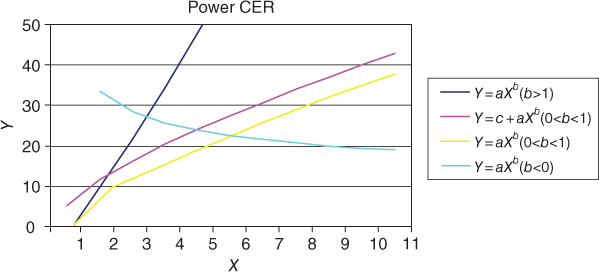
Figure 4.8 Power CERs
4.3.2.3.3 Exponential CER with Fixed and Variable Cost
Another functional form that is sometimes used to create cost estimating relationships is the exponential form. Figure 4.9 illustrates the various shapes an exponential CER can take in modeling a cost relationship.
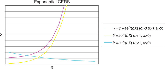
Figure 4.9 Exponential CER
4.3.2.3.4 Logarithm CERs
Finally, another form that may be useful for describing the relationship between cost and a particular independent variable is the logarithmic CER. The shape for a logarithmic CER for a couple of functional forms is provided in Figure 4.10.
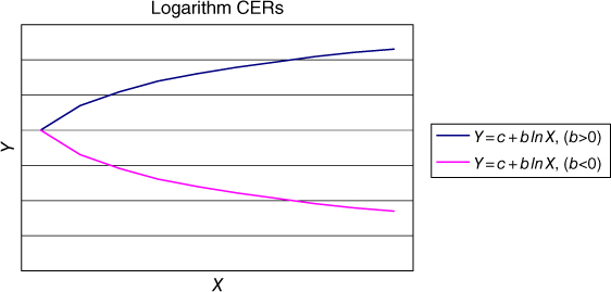
Figure 4.10 Logarithm CER
4.3.2.4 Constructing a Cost Estimating Relationship
As mentioned earlier, in order to construct a CER, we need enough data to adequately fit the appropriate curve. What is adequate is determined by the cost analysts and is a judgmental decision that is largely driven by what data is available. For most of the previous CER model forms, a minimum of three or four data points are sufficient to be able to construct a CER. Unfortunately, a CER constructed from so few points is likely to have a significant amount of error associated with it. Ordinarily, linear regression is used to construct the CER. Linear regression can be used on all of the functional forms by transforming the data in order to establish a linear relationship. Table 4.9, adapted from Stewart et al. (1995), illustrates the relationship between the various CERs and the transformations necessary in order to estimate the parameters for the CER using linear regression.
Table 4.9 Linear Transformations for CERs
| Linear | Power | Exponential | Logarithmic | |
| Equation form desired | Y = a + bX | Y = axb | Y = aebX | Y = a + b ln X |
| Linear equation form | Y = a + bX | lnY = ln a + blnX | lnY = ln a + bX | Y = a + b ln X |
| Req'd data transform | X,Y | lnX,lnY | X, ln Y | ln X,Y |
| Regression coef obtained | a,b | ln a,b | ln a,b | a,b |
| Coef reverse transform req'd | None | EXP(ln a),b | EXP(ln a),b | None |
| Final coef | a,b | a,b | a,b | a,b |
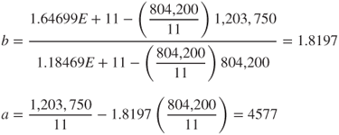
Once the data has been appropriately transformed, linear regression is used to estimate the parameters for the CERs by fitting a straight line through the set of transformed data points. Least squares is used to determine the coefficient values for the parameters a and b of the linear equation. The parameters are determined by using the following formulas:
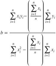
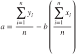
Most of the time, especially when we have a reasonable size data set, a statistical analysis package such as Excel, Mini-Tab, JMP, or R may be used to perform the regression analysis on the data.
Example: Suppose we have collected the following data on square footage and construction costs for a manufacturing facility in Table 4.10. Establish a CER between square footage and facility cost using the data provided. Analyze the data using a linear model.
Table 4.10 Square Footage and Facility Costs for Manufacturing Facility Construction
| X | Y |
| Square Footage | Cost ($) |
| 240,000 | 450,000 |
| 17,500 | 35,000 |
| 24,000 | 42,000 |
| 5,500 | 14,000 |
| 7,000 | 16,000 |
| 57,500 | 105,750 |
| 125,000 | 225,000 |
| 35,000 | 69,000 |
| 89,700 | 185,000 |
| 27,000 | 62,000 |
| 176,000 | 310,000 |
We will fit the data to a simple linear model. Figure 4.11 is a regression plot of the data with a regression line fit to the data.
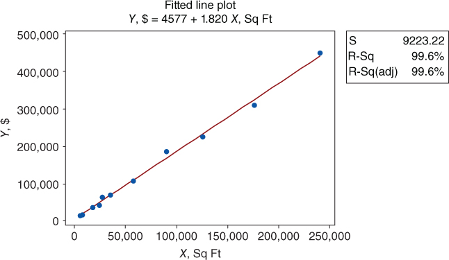
Figure 4.11 Regression plot
We can estimate the parameters for a line that minimizes the squared error between the line and the actual data points. If we summarize the data, we get the following:
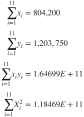
Using the summary data, we can calculate the coefficients for the linear relationship.
If we enter the same data set into Mini-Tab, we obtain the following output:
Examining the output, we see that the model is significant and that it accounts for approximately 99% of the total variation in the data. We note that the intercept term has a p-value of 0.273 and therefore could be eliminated from the model. As part of the analysis, one needs to check the underlying assumptions associated with the basic regression model. The underlying assumption is that the errors are normally distributed, with a mean of zero and a constant variance. If we examine the normal probability plot (Figure 4.12) and the associated residual plot (Figure 4.13), we see that our underlying assumptions seem reasonable. We see that the residual data fall along a relatively straight line, passing the “fat pencil” test, and therefore are probably normally distributed. Second, it appears that the variance of the residuals has a mean value of zero, and the variance appears to be relatively constant for this small sample.
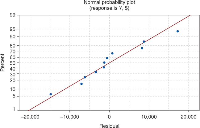
Figure 4.12 Normal probability plot
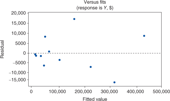
Figure 4.13 Residual plot
4.3.2.5 Cost Estimating Relationship Examples
In this section, we provide several examples of hypothetical CERs that could be used to assemble a cost estimate for the air vehicle component of the UAV system described in the WBS given in Table 4.8. To estimate the unit production cost of the UAV air vehicle component, we sum the first unit costs for the propulsion system, the guidance and control system, the airframe, the sensor payload, and the associated Integration and assembly cost. Suppose the system that we are trying to estimate the first unit production cost has the following engineering characteristics:
- Requires 1300 lbs of thrust
- Requires a 32 GHz guidance and control computer
- Has a 3-in. aperture on the antenna, operating in the narrow band
- Airframe weight of 500 lbs
- Payload weight of 25 lbs
- System uses electro-optics
- System checkout requires nine different test procedures
Suppose the following CERs have been developed using data from five different missile programs and one UAV program during the last 10 years.
4.3.2.5.1 Propulsion CER
The following CER was constructed using the propulsion costs from four of the five missile programs and the one UAV program. Two of the missile programs were excluded because the technology used in those programs was not relevant for the system currently being estimated. The CER for the propulsion system is given by
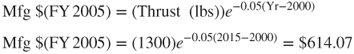
The manufacturing cost in dollars for the propulsion system is a function of thrust as well as the age of the motor technology (current year minus 2000).
4.3.2.5.2 Guidance and Control CER
The guidance and control CER was constructed using data from the two most recent missile programs and the UAV program. This technology has evolved rapidly, and it is distinct from many of the early systems. Therefore, the cost analysts chose to use the reduced data set to come up with the following CER:
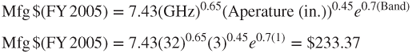
The manufacturing cost in dollars for the guidance and control system is a function of the operating rate of the computer, the diameter of the antenna for the radar, and whether or not the system operates over a wide band (0) or narrow band (1).
4.3.2.5.3 Airframe CER
Suppose the following CER was constructed using the airframe cost data from the five missile programs and one UAV program. The CER for the airframe is given by
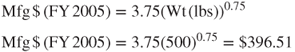
Thus, the manufacturing costs in dollars for the airframe can be estimated if the analyst knows or has an estimate of the weight of the UAV airframe.
4.3.2.5.4 Payload Sensor System
The following CER was established using data from two of the previous missile programs and the UAV program. The payload sensing system being estimated is technologically similar to only two of the previous missile development efforts and the UAV program.
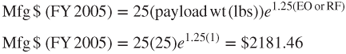
The manufacturing cost for the sensing system in dollars is a function of the weight of the payload and the type of technology used. The term EO/RF is equal to 1 if it uses electro-optic technology and 0 if it uses RF technology.
4.3.2.5.5 Integration and Assembly
This represents the costs in dollars associated with integrating all of the UAV air vehicle components, testing them as they are integrated, and performing final checkout once the UAV air vehicle has been assembled.
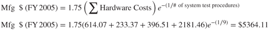
4.3.2.5.6 Air Vehicle Cost
Using this information, the first unit cost of the UAV air vehicle system is constructed as follows:
This cost is in fiscal year 2005 dollars and it must be inflated to current year dollars (2015) using the methods discussed in Section 4.3.4. Once, the cost has been inflated, the initial unit cost can be used to calculate the total cost for a purchase of 500 UAV air vehicles using an appropriate learning curve as discussed in the next section.
4.3.3 Learning Curves
Learning curves are an essential tool for modeling the costs associated with the manufacture of large quantities of complex systems. The “learning” effect was first noticed when analyzing the costs of airplanes in the 1930s (Wright, 1936). Other manufacturing sectors have found similar “learning” effects whereby human performance improves by some constant amount each time the production quantity is doubled (Thuesen & Fabrycky, 1989). For labor-intensive processes, each time the production quantity is doubled, the labor requirements necessary to create a unit decrease by a fixed percentage of their previous value. This percentage is referred to as the learning rate.
Typically, each time the production quantity is doubled, a 10–30% cost or labor saving is achieved (Kerzner, 2006). This l0–30% saving equates to a 90–70% learning rate. This learning rate is influenced by a variety of factors, including the amount of preproduction planning, the maturity of the design of the system being manufactured, the level of training of the production workforce, the complexity of the manufacturing process, as well as the length of the production run. Figure 4.14 shows a plot of a 90% learning rate and a 70% learning rate for a task that initially takes 100 h (Parnell et al., 2011). As evidenced by the plot, a 70% learning rate results in significant improvement of unit task times over a 90% curve. Typical learning rates by industry are given as follows (Stewart et al., 1995):
- Aerospace – 85%
- Repetitive electronics manufacturing – 90–95%
- Repetitive machining – 90–95%
- Construction operations – 70–90%.
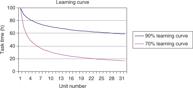
Figure 4.14 Plot of learning curves (Source: Parnell et al. 2011. Reproduced with permission of John Wiley & Sons)
4.3.3.1 Unit Learning Curve Formula
The mathematical formula for the learning curve shown in Figure 4.14 is given by
where
 = the cost or time required to build the
  unit
unit = the cost or time required to build the initial unit
 = the number of units to be built
 = negative numerical factor, which is derived from the learning rate and is given by
4.9
= negative numerical factor, which is derived from the learning rate and is given by
4.9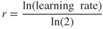
Typical values for r are given in Table 4.11.
Table 4.11 Factors for Various Learning Rates
| Learning Rate (%) | Factor, r |
| 95 | −0.074 |
| 90 | −0.152 |
| 80 | −0.322 |
| 70 | −0.515 |
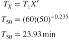
The total time required to produce all units in a production run of size N is given as follows:
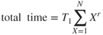
Using the aforementioned equation, with an r-value of −0.152 for a 90% learning rate, we can calculate the unit cost for the first four items. Assuming an initial cost of $100, Table 4.12 provides the unit cost for the first four items as well as the cumulative average cost per unit required to build X units. Figure 4.15 plots the Unit Cost curve and the Cumulative Average cost curve for a 90% learning rate for 32 units.
Table 4.12 Unit Cost and Cumulative Average Cost
| Total Units Produced | Cost to Produce Xth Unit | Cumulative Cost | Cumulative Average Cost |
| 1 | 100 | 100 | 100 |
| 2 | 90 | 190 | 95 |
| 3 | 84.6 | 274.6 | 91.53 |
| 4 | 81 | 355.6 | 88.9 |
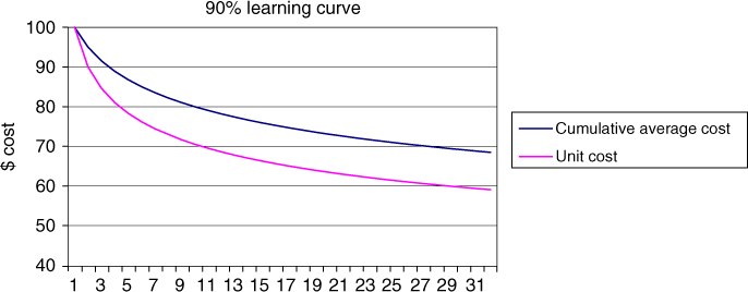
Figure 4.15 Ninety percent learning curve for cumulative average cost and unit cost for 32 units
When using data constructed with a learning curve, the analyst must be careful to note whether they are using cumulative average data or unit cost data. It is easy to derive one from the other, but it is imperative to know what type of data one is working with to calculate the total system cost correctly. Note that the cumulative average curve is above the unit cost curve.
First, the task is assumed to have an 80% learning rate because the cost of the second unit is 80% of the cost of the first. If we double the output again, from 2 to 4 units, then we would expect the fourth unit to be assembled in (48 min) × (0.8) = 38.4 min. If we double again from four to eight units, the task time to assemble the 8th wing assembly is (38.4) × (0.8) = 30.72 min.
First, we need to define r for an 85% learning rate:
Given r, we can now determine the assembly time for the 50th wing assembly as follows:
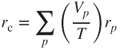
4.3.3.2 Composite Learning Curves
Many new systems are often constructed using a variety of processes, each of which may have their own unique learning rate. A single composite learning rate can be constructed that characterizes the learning rate for the entire system using the rates of the individual processes. Stewart et al. (1995) use an approach that weights each process in proportion to its individual dollar or time value. Using this approach, the composite learning curve is given by
where
 = composite learning rate
 = learning rate for process p
 = value or time for process p
- T = total time or dollars for system.
4.3.3.2.1 Approximate Cumulative Average Formula
The formula for calculating the approximate cumulative average cost or cumulative average number of labor hours required to produce X units is given by
This formula is accurate within 5% when the quantity is greater than 10.
4.3.3.3 Constructing a Learning Curve from Historical Data
The previous formulas are all dependent upon having a value for the learning rate. The learning rate can be determined from historical cost and performance data. The basic data requirements for constructing a learning rate include the dates of labor expenditure, or cumulative task hours, and associated completed units.
By taking the natural logarithm of both sides of the learning curve formula, one can construct a linear equation, which can be used to find the learning rate.
The intercept for this linear equation is ![]() and the slope of the line is given by r. Given r, the learning rate can be found using the following relation:
and the slope of the line is given by r. Given r, the learning rate can be found using the following relation:
This is best illustrated through an example.
Transforming the data by taking the natural logarithm of the cumulative units and associated cumulative average hours yields Table 4.14.
Table 4.14 Natural Logarithm of Cumulative Units Completed and Cumulative Average Hours
| Cumulative Units Completed X | ln X | Cumulative Average Hours TX | ln TX |
| 1 | 0 | 100 | 4.60517 |
| 2 | 0.693147 | 95 | 4.55388 |
| 3 | 1.098612 | 86.66 | 4.46199 |
| 4 | 1.386294 | 80 | 4.38203 |
| 5 | 1.609437 | 72 | 4.27667 |
| 6 | 1.791759 | 66.67 | 4.19975 |
Figure 4.16 is a plot of the transformed data. Performing linear regression on the transformed data yields the following values for the slope and intercept of the linear equation.
| Slope | r = −0.2253 |
| Intercept | ln T1 = 4.660 |
| Coefficient of determination | R2 = 0.897 |
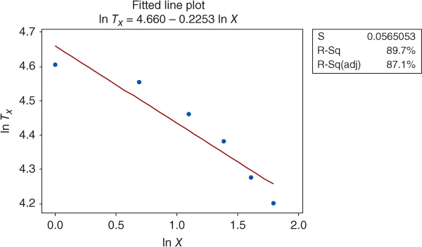
Figure 4.16 Fitted line plot
Thus, the learning rate is determined using the following relationship:
4.3.4 Net Present Value
To help assess the potential economic benefits of a system to an organization, Net Present Value (NPV) is often used to calculate the present worth from a system or process based on the summation of cash flows over its lifetime. It differs in other metrics such as Return on Investment (ROI) and its more complex metric Internal Rate of Return (IRR), which are finance metrics and which do not account for risk by including the discount rate. If an NPV for a program is negative, this indicates that the program is not fiscally profitable. If the NPV is positive, it indicates that the program has a good chance of being profitable. Cash flow within the initial 12 months is not discounted for the purpose of calculating NPV. In most cases, the cash flow for the first year is often negative because of initial investments (Khan, 1999). A program's NPV can also be calculated for a prescribed period of time (e.g., 5, 10, or 15 years). This is done when comparing programs with different life expectancies or if attempting to assess when a program becomes profitable.
Calculation of the NPV requires the inclusion of annual inflation and discount/interest rates. Selecting an appropriate discount rate for calculating NPV is an area of continuing research. Example discount rates that may be applicable for calculation of NPV include but are not limited to the following:
- Hurdle Rate – often calculated by evaluating existing opportunities in operations expansion, rate of return for investments, and other factors deemed relevant by management
- Internal Rate of Return (IRR) or Economic Rate of Return (ERR) – the “annualized effective compounded return rate” or rate of return that makes the NPV of the cash flow for a particular investment or project equal to zero
- Weighted Average Cost of Capital (WACC) – the average rate an organization expects to pay to each of its security holders to back the effort
For each year, one must assess the expected value of the year's cash flow (CF) by the inflation and interest rate to normalize the values to a common year. The first step is to calculate the annual cash flow (ACF) or net cash value (NCV) for each year for the program. The ACF is the value of revenues and expenditures of the program for a discrete period of time (e.g., monthly or annually). Revenue can include payments to the program for products or services delivered. Expenses include all cost associated with the effort. A formula for calculating ACF is
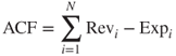
where
 = Annual Cash Flow (i.e., Net Cash Value)
 = Revenue
 = Expenditure
 = Expenditure or revenue
 = Total number of expenditure and revenues for the year.
This can be done by first adjusting for the inflation rate and then adjusting for interest during the calculation of the NPV. Forecasted expenditures and returns are adjusted to the current year's currency value or the annual cash flow after inflation (CFAI) or present value (PV). This is also known as net cash flow. To adjust the expected value of the year's CF by the inflation and interest rate to its current value, the following formula can be used:
where
 = Cash Flow after Inflation (i.e., Present Value (PV))
 = Annual Cash Flow (i.e., Net Cash Value)
 = Expected Rate of Inflation for the End of Year (EOY)
 = End of Year (EOY) for the program (0, …, n)
Summing the CFAI without accounting for the annual interest rate produces the Discounted Cash Flow (DCF). However, to get a more accurate account for the risk associated with the program, include the interest rate in our summation calculations to generate the NPV. The following equation calculates the NPV by summing the CFAIs for the program after adjusting each for the annual interest rate (Khan, 1999).2
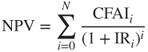
where
 = Net Present Value
 = Cash Flow after Inflation (i.e., Present Value (PV))
 = Interest Rate for the year (time period)
 = End of Year (EOY) for the program (0,…,n)
 = Total number of years (time periods)
Table 4.15 is an example spreadsheet used to show the calculations of the NPV for a program that has an initial investment of $250,000.00 to retool the factory, $ 52,000.00 annual cost for recurring costs, $86,000.00 in estimated annual sales, and $109,000.00 is expected for recapitalization of facilities and equipment after 7 years. The annual interest is 3%, and the estimated annual inflation rate is 7%.
Table 4.15 Example Net Present Value Calculations
| EOY | Cash Outflows ($) | Cash Inflows ($) | Net Cash Value ($) | Inflation (%) | Interest (%) | Cash Flow after Inflation (CFAI) ($) | Cash Flow Interest ($) | EOY Summation ($) |
| 0 | (−) 250,000.00 | (−) 250,000.00 | 3 | 7 | (−) 250,000.00 | (−) 250,000.00 | (−) 250,000.00 | |
| 1 | (−) 52,000.00 | 86,000.00 | 34,000.00 | 3 | 7 | 35,020.00 | 32,729.69 | (−) 217,270.31 |
| 2 | (−) 52,000.00 | 86,000.00 | 34,000.00 | 3 | 7 | 36,071.00 | 31,504.41 | (−) 185,765.90 |
| 3 | (−) 52,000.00 | 86,000.00 | 34,000.00 | 3 | 7 | 37,152.00 | 30,327.18 | (−) 155,438.72 |
| 4 | (−) 52,000.00 | 86,000.00 | 34,000.00 | 3 | 7 | 38,267.00 | 29,193.89 | (−) 126,244.83 |
| 5 | (−) 52,000.00 | 86,000.00 | 34,000.00 | 3 | 7 | 39,416.00 | 28,103.61 | (−) 98,141.22 |
| 6 | (−) 52,000.00 | 86,000.00 | 34,000.00 | 3 | 7 | 40,599.00 | 27,051.11 | (−) 71,090.11 |
| 7 | (−) 52,000.00 | 195,000.00a | 143,000.00 | 3 | 7 | 175,876.00 | 109,517.99 | 38,427.88 |
| NPV at EOY 7 | 38,427.88 |
a $86,000.00 + $109,000.00 = $195,000.00.
Many computer-based spreadsheet programs have built-in formulas for ROI, IRR, and NPV. Each spreadsheet calculates NPV using a similar if not exact same methodology; however, they may differ from how you wish to calculate NPV or how you need to reference your raw data. Thus, ensure that you read how each automated spreadsheet calculates NPV. There are also numerous web-based NPV calculators to help you calculate these values and ensure you that understand if you need to precalculate the NCV or ACF for these online calculators.
NPV can be assessed as an aggregate sum of cash flow, individual program resources, or cost categories (e.g., people, facilities, and costs; direct and indirect costs; or science and technology, procurement, and operations and sustainment/maintenance). Figure 4.17 is an example of a tornado chart of the NPV of a 7-year program described in Table 4.15. Tornado charts vary each variable from low to base to high while holding all other variables at their base value. System expenditures and revenue are broken down by direct and indirect cost categories. The chart provides the ability to see where the major cost drivers and savings are for the program. One can see that the largest predicted costs are Acquisition Costs for the worst-case (high-case) scenario. The lowest costs are Indirect Costs for the low-case (best-case) scenario. In this example, the lower cost case also has the higher Sales and Recapitalization predictions. The Base Case and the Lower Costs and Higher Sales forecast a positive NPV for the program after 7 years. The Inflation and Interest rates used for the calculations are seen in Table 4.16.
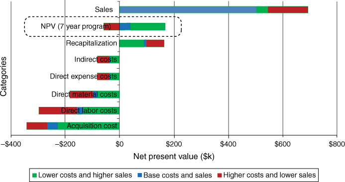
Figure 4.17 Example net present calue (NPV) tornado chart for a 5-year program
Table 4.16 Example Net Present Value Inflation and Interest Rates
| Case | Inflation (%) | Interest (%) |
| Lower costs and higher sales | 1.0 | 9.0 |
| Base costs and sales | 3.0 | 7.0 |
| Higher costs and lower sales | 9.0 | 1.0 |
As a value based on expected future conditions, uncertainty is involved in the calculation on NPV. This uncertainty should be assessed against each of the annual values: expenditures, cash inflow, inflation, and interest. This provides the ability to illustrate the expected best case, worst case, and most likely NPV for a planned investment. Figure 4.18 provides an example of a hurricane chart of the annual cumulative NPV forecast for the program outlined in Table 4.15. The deviation is based on a max and a min range of inflation and interest rates used to calculate the best- and worst-case values with the midline calculation based on the most likely value for each (Table 4.16). The pie charts indicate the percentage of recurring and nonrecurring costs. The size of each pie chart indicates the magnitude of total costs incurred. Although NPV is calculated for the lifetime of the program, the hurricane chart provides an illustration of the annual level of financial risk incurred for the program. The chart indicates that in the worst case, NPV is never positive. In the best case, the NPV is positive starting at EOY 5. The likely case indicates that positive NPV occurs at the end of the program after recapitalization of facilities and equipment.
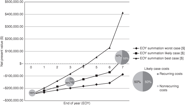
Figure 4.18 Example cumulative net present value hurricane chart
When comparing the NPV of multiple options or systems, two conditions must be met (Park, 2004):
- Each system assessed must be mutually exclusive of the other (i.e., the choice of one system or alternative must not include the other).
- The lifetime of each system must be the same. If the duration of the lifetime differs between each system, then use the shortest.
4.3.5 Monte Carlo Simulation
Monte Carlo analysis is a useful tool for quantifying the uncertainty in a cost (or NPV) estimate. In Section 3.5.2, Monte Carlo Modeling is introduced and the details associated with building a Monte Carlo simulation model are summarized in Figure 3.9. For a cost model, the Monte Carlo process rolls up all forms of uncertainty in the cost estimate into a single probability distribution that represents the potential system costs. Given a single distribution for cost, the analyst can characterize the uncertainty and resulting risk associated with the cost estimate and provide management with meaningful insight about the cost uncertainty of the system being studied. Kerzner (2006) provides five steps for conducting a Monte Carlo analysis for models. Kerzner's five steps are as follows:
- Identify the appropriate WBS level for modeling; as the system definition matures, lower level WBS elements can be modeled in the cost model.
- Construct an initial estimate for the cost for each of the WBS elements in the model.
- Identify those WBS elements that contain significant levels of uncertainty. Not all elements will have uncertainty associated with them. For example, if part of your system has off-the-shelf components and you have firm-fixed-price quotes for the material, then there would be no uncertainty with the costs for those elements of the WBS.
- Quantify the uncertainty for each of the WBS elements with an appropriate probability distribution. Often times, a triangular distribution is used for the first estimate.
- Aggregate all of the lower level WBS probability distributions into a single WBS level 1 estimate by using a Monte Carlo simulation yielding a cumulative probability distribution for the system cost. This distribution can be used to quantify the cost risk as well as identify the cost drivers in the system estimate.
Kerzner (2006) points out that caution should be taken when using Monte Carlo analysis. As with any model, the results are only as good as the data used to construct the model; “garbage in, yields garbage out” applies to this situation. The specific distribution used to model the uncertainty in WBS elements depends on the information available. As mentioned earlier, many cost analysts default to the use of a triangle probability distribution to express uncertainty. Kerzner (2006) suggests that the probability distribution selected should fit some historical cost data for the WBS element being modeled. When only the upper and lower bounds on the cost for a WBS element are available, a uniform distribution is frequently used in a Monte Carlo simulation to allow all values between the bounds to occur with equal likelihood. The triangular distribution is often adequate for early life cycle estimates where minimal information is available (lower and upper bounds) and an expert is available to estimate the likeliest cost. As the system definition matures, and relevant cost data becomes available, other distributions, such as the Beta distribution, could be considered and the cost estimate updated.
Example: We will continue with our example of estimating the cost for a hypothetical UAV. One key element of the UAV system is estimating the software nonrecurring costs for the system. The following CERs have been developed to estimate the cost of the ground control software for the UAV system based on several previous UAV development efforts, and the mission–embedded flight software relationship is estimated using information from the conceptual design phase of the UAV system. Software development costs are often a function of its complexity and size.
Ground Station Software
Embedded Flight Software
The DoD parameter equals 1 if it is a DoD UAV, and 0 otherwise. Since the UAV under consideration is a commercial UAV, the DoD parameter is set equal to 0. EKSLOC is a measure of the size of the software coding effort measured in thousands of source lines of code. During design and development, engineers need to estimate these sizes for their project. Assume that it is early in the design process and the engineers are uncertain about how big the coding effort is. After talking with the design engineers, the cost analyst has chosen to use a triangular distribution to estimate the EKSLOC parameter. The analysts ask the design expert to provide several estimates; an estimate of the most likely number of lines of code, m, which is the mode, and two other estimates, a pessimistic size estimate, b, and an optimistic size estimate, a. The estimates of a and b should be selected such that the expert believes that the actual size of the source lines of code will never be less (greater) than a (b). These become the lower and upper bound estimates for the triangular distribution. Law and Kelton (1991) provide computational formulas for a variety of continuous and discrete distributions. The expected value and variance of the triangular distribution are calculated as follows:
Suppose our expert defines the following values for EKSLOC for each of the software components.
| Software Type | Minimum Size Estimate (KSLOC) | Most Likely Size Estimate (KSLOC) | Maximum Size Estimate (KSLOC) |
| Ground Station Software | 10 | 20 | 35 |
| Embedded Flight Software | 5 | 15 | 25 |
Using these values and the associated CERs, a Monte Carlo analysis is performed using @Risk (Palisade Corporation, 2014) software package designed for use with Excel. The probability density function for the embedded flight software is shown in Figure 4.19.
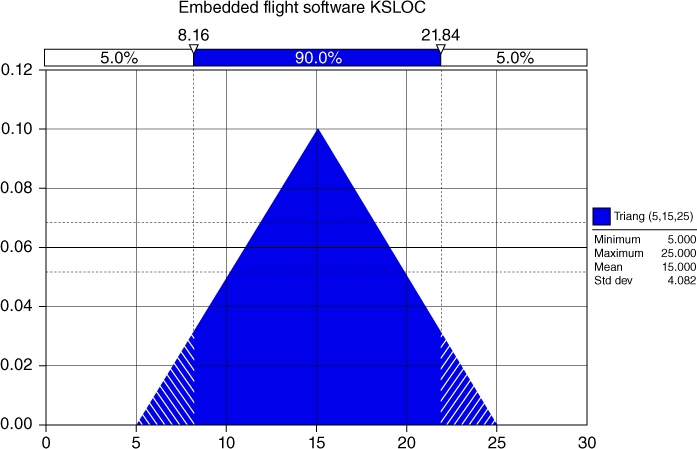
Figure 4.19 Triangular distribution for embedded flight software
The PDF for the estimated labor hours is given in Figure 4.20 for 10,000 simulation runs.
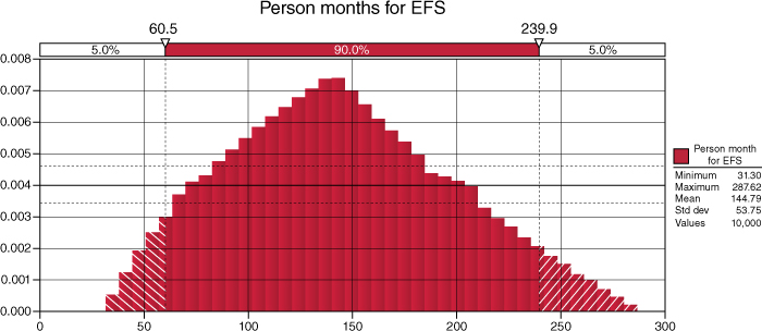
Figure 4.20 PDF for total person-months for embedded flight software development
Finally, suppose that management is uncertain about the labor cost for software engineers. Management believes the labor cost is distributed as a PERT random variable with a minimum of $25, a maximum of $60, and a most likely value of $35. The PDF and CDF for the total software development cost are given as follows. This estimate assumes that engineers work 36 h in a week on coding and that there are 4 weeks in a month.
The primary observation to make from Figure 4.21 is the spread in possible software development costs due to the uncertainty assumptions imposed on the WBS elements when the Monte Carlo simulation was constructed. For this example, while it is more likely that the actual software development costs will clump around $1.3 million, it is possible for them to be more than two times as much or as little as 500 k because of this uncertainty. In the former case, the project could be threatened; in the latter, the project would continue well within the budget.
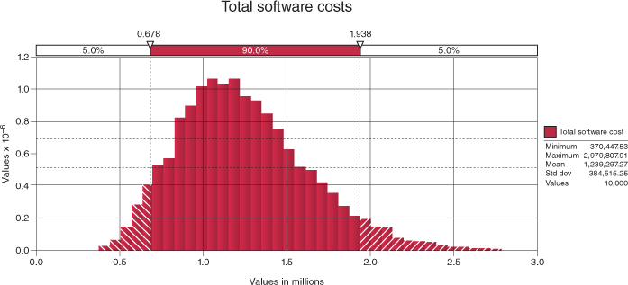
Figure 4.21 PDF for software development cost
Once we have the PDF for the cost of development, we can construct the CDF to calculate the probability that the cost of the software development is less than x. Applications such as @Risk accomplish this task easily. Figure 4.22 contains the CDF for the total software development costs.
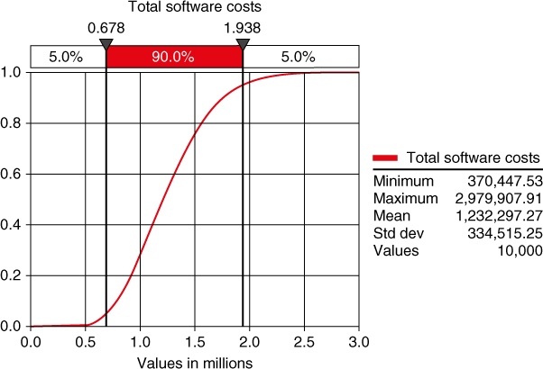
Figure 4.22 CDF for total software development costs
Using the CDF, we can make probability statements related to the software development cost. For example, we can state that there is a 50% probability that the software development costs will be less than $1.295 million; similarly, there is a 5% probability that the software development costs will exceed $1.938 million. This information is useful to senior-level management as they assess the costs risks associated with the development program.
4.3.6 Sensitivity Analysis
As discussed in Section 3.5.2, sensitivity analysis can be conducted on the Monte Carlo Simulation model. Specifically, the results can be analyzed to identify those elements that are the most significant cost drivers. In our example, it is relatively easy as our total cost is only a function of two cost elements and one other factor. But realistic cost estimates may have on the order of 10–50 cost elements/factors and choosing the cost drivers from this set is not so easy. Fortunately, @Risk provides a tool that analyzes the relative contribution of each of the uncertain components to the overall cost and variance for the system estimate. Figure 4.21 shows the sensitivity output for this example.
Examining the chart in Figure 4.23, the uncertainty associated with “Embedded Flight Software Person-Months” (EFKSLOC) is the main contributor to the variability in the total software cost estimate, followed by the uncertainty in labor rate for software engineers. The cost analysis should consider spending more time getting a better estimate for the cost risks associated with the “embedded flight software person-months” since reductions in the uncertainty associated with this WBS element will have the greatest impact on reducing the variability in the total cost estimate seen in Figure 4.21. Better estimates on the labor rate will also substantially reduce the uncertainty in the total system costs.
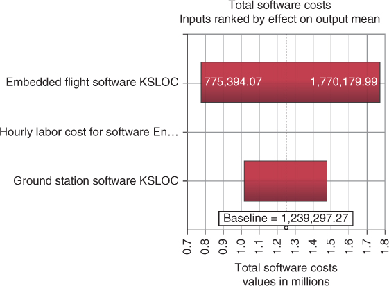
Figure 4.23 Sensitivity chart
4.4 Affordability Analysis
Building on the resource assessment and cost analysis described earlier, organizations typically desire to understand the impact of cost, performance, risk, and resource allocation in the context of the portfolio of activities and competing priorities. For industry, affordability is the ability to develop a product or provide a service at a profit that balances performance and cost. For government organizations such as DoD, a product or program is affordable if it balances cost, performance, and risk while meeting their missions. This section discusses the background of developing affordability analysis, a comparison of cost analysis and affordability analysis, some affordability-related definitions and provides background, definitions, and a framework for conducting affordability analysis.
4.4.1 Background
In 2009, Congress passed the Weapon System Acquisition Reform Act (WSARA) to improve the way DoD contracts and purchases major weapons systems. The law established the Office of Cost Assessment and Program Evaluation (CAPE) and established reforms that were expected to save billions of dollars. As the WSARA formally demanded more fidelity and rigor in acquisition analysis, leaders in DoD asked the Military Operations Research Society (MORS) to engage the Acquisition and Analysis Communities to share and develop a set of best practices that address risk assessment and trade space analysis in support of acquisition. In September 2011, MORS held the workshop “Risk, Trade Space & Analytics in Acquisition,” to determine and share a set of best practices for those significant analytical challenges that arise during the acquisition process. One significant conclusion from that workshop was that “affordability analysis” was poorly defined across the community. Leaders in DoD asked MORS for help with definitions and procedures.
In October 2012, MORS conducted an “Affordability Analysis: How Do We Do It?” workshop where the following was learned: (i) no organization was responsible for affordability analysis (OSD-ATL is only responsible for affordability); (ii) every organization defines affordability analysis and conducts it differently; and (iii) there was no process to follow to conduct affordability analysis. In February 2013, the MORS Affordability Analysis Community of Practice (AA CoP) was formed with members from across government, industry, and academia to continue the research from the October 2012 workshop and develop a “how-to” manual, process, or guide for affordability analysis.
4.4.2 The Basics of Affordability Analysis Are Not Difficult
Let us start with an example to put affordability analysis in perspective. A couple makes $100,000 per year. They see a nice house for $500,000. “Can we afford that?” they ponder. We all know that it depends. It depends on what fraction of their budget they can allocate to the house, the payment terms of the house itself (interest rate, down payment required, etc.), their need for the house, the added value they derive from the house (e.g., utility, change in life style), and the degree to which the individual is willing to give up other budget items so that funds can be allocated to the house.
To summarize, the following are the things you need to know to buy a house:
- Need for house
- Fraction of budget available for house purchase
- Payment terms
- Willingness to give up other spending
While the answer to the couple's question involves several variables, with a few facts, the answers to their questions can generally be figured out with some home-buying analyses. The Department of Defense (DoD) needs a similar capability for affordability analyses, that is, the ease of knowing when something is outside of the fiscally possible. As shown as follows, the things needed to determine affordability-related decisions are related to the things needed to answer whether or not to buy a house.
Following are the things you need to know for affordability decisions:
- Needs and priorities
- Fraction of budget available for need(s)
- Basis of payment (Cost)
- Overall capability implications
As you read the information needed for buying a house and affordability decisions, you can see that affordability analysis is much more than just a straightforward cost analysis. The DoD has the directives to be effective and efficient, but struggles with the dynamic capability (i.e., a force that stimulates change or progress within a system or process) to use affordability as a guide to maximize value within operational, technical, and fiscal constraints. For an affordability analysis to be useful, it must be actionable: it must lead to a well-informed decision or support a specific action, such as a program start or cancellation, or perhaps a new operating concept that provides needed capability at reduced cost.
The remaining paragraphs in this section are DoD-specific. Affordability analysis efforts were started at the request of DoD Leadership and the work completed was conducted by representatives in the DoD, Defense Contractors, and Defense-related academia responding to the request. However, the affordability analysis definitions and framework in this section could be adapted for non-DoD/commercial work similarly to the house buying example.
4.4.3 DoD Comparison of Cost Analysis and Affordability Analysis
From the 2012 MORS Workshop on “Affordability Analysis: How Do We Do It?,” consensus of the attendees was that clarity of definition, sufficiency criteria, and regulatory policy were consistently absent from affordability analysis. Affordability was determined not to be a number, but a decision, and may vary depending on the stakeholder or the decision maker (i.e., affordability is in the eye of the beholder). (Michealson, “Big A” Affordability Analysis, May 27, 2015). For example, differences could be:
- Size dimension: DoD, service, mission area, or system
- Measurement dimension: Dollars, lives, or time
- Phase dimension: Requirement, acquisition, or operation
When one conducts cost analysis, the process is normally straightforward; analysts have established guidelines and principles to follow. However, when conducting affordability analysis, approaches vary dramatically. Guidance, processes, and institutional acceptance are needed though tools and methodologies were not considered the binding constraints; without them, there will be varying perspectives on affordability.
Since participants were familiar with current costing techniques, the following definitions were developed during the October 2012 Workshop to provide a foundation for an affordability analysis process:
- Cost Analysis primarily considers the monetary and financial aspects of an acquisition – whether it is acquisition cost, design cost, and/or total ownership cost. Individual cost elements of a system or platform are investigated, estimated, and accumulated to arrive at an overall cost.
- Cost–Benefit Analysis compares cost of numerous alternatives to the benefits they provide to inform the course of action selection.
- Capabilities-Based Assessment is a Joint Capabilities Integration Development System (JCIDS) activity designed to identify and prioritize capability gaps and risks.
It was agreed that none of these are affordability analysis, but they all contribute to affordability analysis. Cost analysis provides the basis for costs used in an affordability analysis. Cost–benefit analysis additionally provides solution advantages, quantifiable and nonquantifiable, which affordability analyses incorporate as value or military worth of the acquisition program. Capability gaps, priorities, and risk output from capabilities-based assessments serve as foundational elements in an affordability analysis. These gaps, priorities, and risks form the basis for evaluating acquisition program costs and benefits against fulfillment of stated capability and reveal how well the acquisition program does or does not satisfy DoD objectives within affordability targets.
As a result of these discussions, in January 2015, the Department of Defense Instruction (DODI) 5000.02 Operation of the Defense Acquisition System, Office of the Secretary of Defense (Acquisition, Technology & Logistics), included an overview on affordability for the first time:
- Affordability analysis and affordability constraints are not synonymous with cost estimation and approaches for reducing costs.
- Cost estimates are generated in a bottom-up or parametric manner and provide a forecast of what a product will cost for budgeting purposes (NOTE from the Naval Center for Cost Analysis that the current wording omits analogy, expert opinion, and extrapolation that are also recognized as cost estimation methods).
- Affordability constraints are determined in a top-down manner.
The updated document discusses cost analysis and the differences between cost analysis and affordability analysis, but it still does not discuss affordability analysis.
4.4.4 Affordability Analysis Definitions
Affordability is an abstract term that most people think they understand but have difficulty defining or explaining. The 2011 MORS Workshop on “Risk, Trade Space & Analytics in Acquisition” revealed a lack of consensus on the definition of affordability and related terms. The MORS AA CoP has developed three key definitions – affordability, affordability analysis, and affordability analysis outcomes. These three terms are critical to understanding why, what, and how tasks are undertaken.
- Affordability. The degree to which the resources being allocated to a capability relative to other uses of those resources reflects (i) the importance, urgency, and satisfaction of mission, strategic investment, and organizational needs, and (ii) a prudent balance of performance, cost, and schedule constraints consistent with the time-phased availability (technical, market, and fiscal) of budgeted resources.
- Affordability Analysis. A process and assessment that supports resource allocation decision-making. It identifies and quantifies the performance expectations of stakeholders, assigns value to those expectations, and measures the LCC of alternatives relative to both opportunity costs and resourcing actions or plans.
- Affordability Analysis Outcomes. Practically, affordability analyses must substantiate resource plans, given a mission scope and a budget scope, while taking advantage of “good buys” and available offsets. Culturally, rewarding the practice and use of affordability analyses should change the conversations of decisions-makers, enabling them to deliver portfolio outcomes that are more effective and efficient while staying within and informing budget boundaries.
In the first MORS Affordability Analysis Workshop, two interpretations of affordability were also developed.
- Affordability in the “large” means assessing whether a mission, task, function, capability, system of systems, program, or initiative – considering what it is going to cost (or is costing us, i.e., the total costs) – provides sufficient value in the context of all of the other things needed (“Big A”).
- Affordability in the “small” means being frugal – being cost-efficient in executing a program, from beginning to end and not being extravagant in choosing capabilities and solutions to challenges; getting the most bang for the buck (“little a”).
As shown in Figure 4.24, the services, contractors, program managers, and others tend to operate in the “little a” realm (i.e., doing things right), while DoD, Congress, and Service leadership usually operate in the “Big A” realm (i.e., doing the right things); the perception is that the majority of “Big A” affordability analysis is conducted by the leadership, while “little a” is conducted by program managers. However, that is not quite true. Both leadership and program managers conduct “Big A” affordability analyses, just at different levels in the enterprise, and the leadership is quite active doing “little a” affordability analyses in late-cycle programs. Additionally, program managers support and influence the leadership's “Big A” work, when requested by (i) initially identifying the right solution at the top level to meet the capability, then (ii) throughout the acquisition life cycle when the customer provides changes/new information is learned conducting a strategic assessment to determine how these new changes affect the mission, task, function, capability, system of systems, program, or initiative – that is, considering the analysis of LCC and performance in relation to alternatives to assess value in the context of other things that are needed.
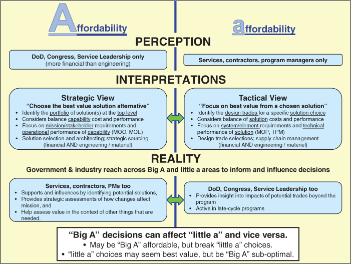
Figure 4.24 “Big A” and “little a” (Source: MORS Affordability Analysis Community of Practice 2015)
As a result, original “Big A” and “little a” affordability interpretations from the first MORS workshop were updated:
- Affordability in the Large:
- Assessing whether a mission, task, function, capability, system of systems, program, or initiative – considering what it is going to cost (or is costing us, i.e., the total costs) – provides sufficient value in the context of all of the other things needed (“Big A”).
- The Strategic View – Identifying the portfolio of solution(s) at the top level, considering LCC and capability/performance in relation to the value provided by other things that are needed.
- Affordability in the Small:
- Being frugal – being cost-efficient in executing a program, from beginning to end and not being extravagant in choosing capabilities and solutions to challenges; getting the most bang for the buck (“little a”).
- The Tactical View – Minimizing costs while maximizing capabilities/performance.
With that said, new elements in a portfolio may be “Big A” affordable and break “little a” choices, and conversely, “little a” choices might seem to be the best value but be “Big A” suboptimal. Affordability in the large is a judgment call. That judgment can change over the life of a program for many reasons, some of which may have absolutely nothing to do with the “little a” of a program. The nature of analysis to support the “A's” differs somewhat due to the nature of the associated questions.
4.4.5 “Big A” Affordability Analysis Process Guide
Since (i) the military services, contractors, and program managers have their own processes for conducting “little a” affordability analysis and (ii) documents developed that are coordinated through a professional society (i.e., MORS) cannot be prescriptive, MORS provided considerations for conducting “Big A” affordability analysis with best practices and lessons learned that are supportive/complementary to all organization's “little a” affordability analysis processes.
The MORS “Big A” Affordability Analysis Process Guide (Michealson, “Big A” Affordability Analysis Process Guide, 2015) seeks to be a thinking construct that allows the DoD, at all institutional levels, to have a data-based conversation about affordability and affordability analysis. The principal goal is not to develop a prescriptive, one-size-fits-all “how-to” manual on doing optimal resource allocations, but to: (i) include outcome and constraint quantification, (ii) consider fiscal stewardship, and (iii) demonstrate how to provide high-efficacy decision support. A secondary purpose is to aid decision-makers or decision-supporters, who have data and may not be experts with analytics. The document proposes a simple set of questions that ensures consideration of key facets, which would have a significant impact on the affordability of a system.
Guidelines for high-quality affordability analysis are offered to include in the life cycle process for understanding, but this construct in no way replaces life cycle management. Sufficiency and quality exit criteria are offered in the affordability analysis process to provide rationale to answer some of the questions expected due to scope design, political motivations, stakeholder motivational considerations, and the complexities with data, tools, and analysis.
The goal is not to develop a prescriptive, one-size-fits-all “how-to” document or a manual on doing optimal resource allocations; the overall goal is to develop an affordability analysis process with best practices, lessons learned, considerations, and so on, as well as including ties to the individual military service's new Affordability Policies and DoD Better Buying Power (BBP) initiatives. BBP has been referred to as DoD's mandate to “do more without more.” BBP is the implementation of best practices to strengthen DoD's buying power, improve industry productivity, and provide an affordable, value-added military capability to the warfighter. Introduced in 2010, BBP is outlined in a series of three memos from the Under Secretary of Defense for Acquisition, Technology and Logistics (ATL). Affordability is a key tenant of BBP 1.0, 2.0, and 3.0 memos, which further strengthens the need for solid, consistent, repeatable affordability analysis practices. BBP mandates affordability as a requirement and enforces affordability caps.
Affordability analysis is essential to establish requirements and caps. BBP states that affordability constraints are to be based on anticipated future budgets for procurement and support of the program. BBP affordability constraints are the artifact of budget, inventory, and product life cycle analysis within a portfolio context. Affordability constraints force prioritization of requirements and drive performance and cost trades to ensure that unaffordable programs do not enter the acquisition process. BBP 3.0 places emphasis on achieving dominant capabilities through innovation and technical excellence and continues with the core theme stating, “Conduct an analysis to determine whether or not a desired product can be afforded in future budgets – before the program is initiated.”
Figure 4.25, the Affordability Analysis Framework, illustrates the question-driven framework that is the basis of the affordability analysis. As shown in the center of the figure, the process is started with the Review Requirements, Needs, and Desired Outcomes Activity and following the arrows working clockwise through the remaining activities: Assess Baseline and Gaps, Determine Feasible Alternatives, and Evaluate Trade-Off Analysis. The bullet questions are subactivities for each activity, and each has several tasks/considerations to help analysts dig for information that assists in drawing conclusions about the affordability of the area or topic in question.
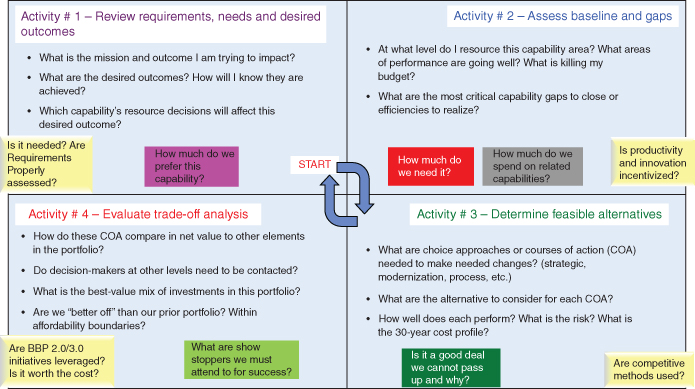
Figure 4.25 Affordability analysis framework (Source: Courtesy of the Military Operations Research Society Affordability Analysis Community of Practice (or MORS AA CoP))
The Review Requirements, Needs, and Desired Outcomes activity sets the stage for the affordability analysis and identifies the resource information readily available by answering the following questions (i.e., the subactivities):
- What is the mission or outcome that will be impacted?
- What are the desired outcomes? How will it be known if they are achieved?
- Which capability's resource decisions will affect the desired outcome?
By answering these questions, this activity (i) generates critical assumptions and shapes the scope of affordability analyses, (ii) identifies analyses needed and the appropriate tradespace to assess, and (iii) affirms that the requirements of the “scope” are properly assessed and capabilities in question are needed. As a result, this activity identifies the resource information readily available and the degree of contention about the AOI.
After an organization has aligned their resources with their goals and targets, they must evaluate their baseline's current resource performance and identify capability gaps. The Assess Baseline and Gaps activity will either identify or validate a mission need and begin the necessary affordability assessments to evaluate alternative resource strategies to meet the emerging needs. Overall, this activity will enable the affordability analysts to understand what is truly needed and incentivize innovation and other high-leverage changes to the baseline by:
- Evaluating baseline performance including baseline effectiveness/performance and cost/affordability of the baseline
- Considering emerging needs that may be driven by many factors to include (i) new or increasing threats, (ii) new responsibilities, roles or missions, (iii) changes in national security objectives, and (iv) aging of resources
- Identifying capability gaps that reflect inability to meet objectives or mission demands and pose risk to accomplishing task and goals
- Considering alternative strategies that not only study new things – platforms/systems/software – that may rectify the gap (problem), but also ways that might change the way business is done in terms of CONOPS, training, doctrine, and so on, to improve the situation.
In the Determine Feasible Alternatives activity, a high-level assessment of affordability of the alternatives proposed helps to gauge which may have more value to the enterprise. As the study of the Affordability options has begun, there is a need to review the alternatives in an analytically rigorous method.
- First, an evaluation the available approaches for desired delta or change (all options) is conducted before addressing any questions of affordability. Are there other possible actions that would result in a change to the bottomline?
- Second, affordability should be included as a key consideration into the design of any solutions. It is easier to assess affordability and affordability options if the environment to study has already been created. The need is to assess alternative capability solutions using proven integrated Capabilities-Based Assessment (CBA) approaches and criteria at a capability level (as opposed to a project level).
The overall goal of this third activity is to determine the feasible solutions to use in the trade-off analysis activity.
The Evaluate Trade-Off Analysis activity focuses on tradespace analysis and a best value evaluation of the affordability assessment in question, to ensure an affordability trade has not been made that produces undesired long-term effects. There are five subactivities associated:
- Prepare for Analysis by checking for completeness of the inputs, normalize data and analysis structures, and evaluate available alternatives.
- Solicit and Determine the Value Structure by analyzing the available information, developing a value framework, and populating the value framework.
- Conduct Trade-Off Analysis by refining candidate portfolios, conducting cost/performance/risk/schedule analysis, conducting the trade-off analysis, and ranking the alternative portfolios.
- Conduct Sensitivity and Risk Analysis by creating a risk and sensitivity analysis methodology and performing risk and sensitivity analysis.
- Make the Decision by preparing to support the decision-maker, creating a “what-if” approach or tool, and supporting the decision-maker assessment process.
In summary, this last affordability analysis activity analytically “proves” which feasible COA from the previous activity is best for the portfolio area (and affects the portfolio). The data or techniques used should provide a better result as the process matures.
After the specific affordability analysis activity and its associated subactivities and tasks are complete, the exit criteria questions help to assess if each specific activity is actually completed, that is, if we are “doing it right” (the gray boxes in each quadrant) as well as “doing the right thing” (the other white boxes in each quadrant). To determine if the affordability analysts are doing the right things, that is, sufficiency, the MORS AA CoP started with the Government Performance and Results Act Modernization Act (GPRAMA—[16 Dec 13]). GPRAMA requests the following from DoD related to affordability and affordability analysis:
- “Provide information on the analytical underpinnings of DoD reasoning with regard to risk-balancing and other trade-offs involved in aligning available departmental resources with national strategy.
- Explain how DoD has considered the element of budget uncertainty.
- Provide information on decision-making about trade-offs between programs and initiatives, in the context of budget constraints.
- Explain more about how “lessons-learned” analysis has been incorporated into strategic planning, particularly with long-standing problem areas such as financial management and cost-containment, and how it will be used in the future.”
As a result, the MORS AA CoP designed their sufficiency exit criteria with the GPRAMA in mind. The affordability analyst can finally get back to the simplicity of the back of the napkin: what are the basic facts that must be known to believe our conclusion? To do this, and support the GPRAMA, five high-level sufficiency criteria support a good affordability analysis for each activity. They are:
- Grounded in a value proposition,
- Addresses the entire life cycle,
- Includes portfolio assessment,
- Is time specific, and
- Contains data-driven analysis.
To ensure that the affordability analyst was doing things right, the MORS Affordability Analysis CoP developed their quality exit criteria:
- Prioritization: The scope and importance of the capability to a relevant value space. How much do we prefer this capability?
- Trade demands: The relative need for the capability and supporting commodities to provide it – an assessment of capability gap severity and criticality. How much do we need it?
- Dollars per capability: The balance in the portfolio must be graphed – dollars relative to other capabilities in the baseline, where investments lie in life cycle, as well as other discriminating characteristics. How much do we spend on related capabilities?
- Cost: An evaluation of net performance/risk/cost bang for the buck; how “buyable” and “best value” is the Course of Action (COA) or option. Is it a good deal we cannot pass up and why?
- Behavioral change required to make COA successful: issues about choices, sunk costs, industrial considerations, or cultural risk factors that may not be quantified; yet, they may preclude success of the initiative; a description of this challenge must be included. What are the showstoppers we must attend to for success?
These exit criteria are critical – if we are not doing it right, or we are not doing the right thing, then the affordability question is a moot point. If we are doing it right, and it is the right thing, then we need to figure out how to pay for it. What can we give up, given the time duration of the capability in question (it may be less than 30 years) and given the array of uncertainties around the cost and value approximation?
Figure 4.26 is a high-level overview product of Lean Six Sigma Value Stream Mapping Activity of the Affordability Analysis Framework described in the question-driven portrayal of Affordability Analysis Framework figure and discussion earlier. This figure shows the activities and artifacts needed to conduct the process and also shows an overview of the “Big A” Affordability Analysis Activities. The “rows” are the four affordability analysis activities and, for each activity, provides an overview of the inputs, process steps (subactivities)/tasks (or considerations), and outputs.
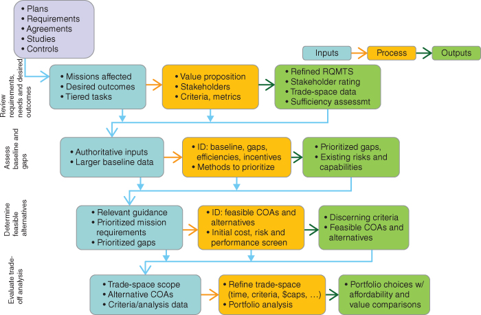
Figure 4.26 Lean six sigma high-level overview product example (Source: Courtesy of the Military Operations Research Society Affordability Analysis Community of Practice (or MORS AA CoP))
As discussed in the framework and process overview, there are five parts for each affordability analysis activity:
- An overview of the activity (with value stream map or process chart)
- The inputs needed for the activity
- The sub-activities for the activity (the framework questions) with associated tasks and considerations
- The exit criteria to complete the activity (sufficiency & quality)
- The outputs from the activity (may not be used by the next activity, could be used by any of the following activities – or available as references).
4.5 Key Terms
- Acquisition Cost: A cost class that includes “the total cost to procure, install, and put into operation a system, product, or special piece of infrastructure. These are the costs associated with planning, designing, engineering, testing, manufacturing, and deploying/installing a system or process” (Parnell et al., 2011, p. 144).
- Affordability: The degree to which the resources being allocated to a capability relative to other uses of those resources reflect (i) the importance, urgency, and satisfaction of mission, strategic investment, and organizational needs, and (ii) a prudent balance of performance, cost, and schedule constraints consistent with the time-phased availability (technical, market, and fiscal) of budgeted resources.
- Affordability Analysis: A process and assessment that supports resource allocation decision-making. It identifies and quantifies the performance expectations of stakeholders, assigns value to those expectations, and measures the LCC of alternatives relative to both opportunity costs and resourcing actions or plans.
- Cash flow (CF): The annual summation of revenues and expenditures for a business, project, or financial product.
- Cost Analysis: The review and evaluation of the separate cost elements and profit or fee in an offerer's or contractor's proposal to determine a fair and reasonable price or to determine cost realism. Cost analysis includes the application of judgment to determine how well the proposed costs represent what the cost of the contract should be, assuming reasonable economy and efficiency (Cost Analysis, 2014).
- Cost: Any term that refers to organizational resource that would be expended for a program/product. Examples include but are not limited to funds, dollars, hours, professional service years, and facility space (Parnell et al., 2011, p. 143).
- Cost Estimation or Estimate: An assessment and forecast of the cost of a hardware, software, and/or services (Williams & Barber, 2011).
- Cost Objective: One of the numerous possible objectives in a value hierarchy; it is often represented as a mathematical value that the organization seeks to minimize. Treated as a separate value and normalized per unit in a tradespace facilitates its presentation to decision makers (Parnell, 2013, p. 141).
- Direct Cost: A cost class that includes costs “that are associated with a specific system, end item, product, process, or service.” These costs can be subdivided into “direct labor, material, or expenses” (Parnell et al., 2011, p. 144).
- Fixed Cost: A cost class that includes costs “that remain constant independent of the quantity or phase of the life cycle being addressed in the estimate.” Examples of fixed costs include “research, lease rentals, depreciation, taxes, insurance, and security” (Parnell et al., 2011, p. 144).
- Indirect Cost: A cost class that includes costs “that cannot be associated with a specific product or process.” These costs can be clustered into an overhead account and applied to “direct costs” as a burden. Examples include “security, accounting and finance labor, janitorial services, executive management, and training” (Parnell et al., 2011, p. 144).
- Learning Curve: A graphical representation of how people and organizations get better at tasks (reduce cost; vertical axis) as experience increases (horizontal axis). (Quantitative Module E: Learning Curves, 2006, p. 772).
- Life Cycle Cost: “The total cost of an alternatece across all stages of the altenative (aquisistion) life cycle.” It normally does not include sunk costs (Parnell, 2013, p. 134 and 146; Parnell et al., 2011, pp. 137–138).
- Monte Carlo: A simulation methodology that is a “realization of a sequence of outcomes by repeated random selection of input scenarios according to experts' probabilities” (Parnell, 2013, p. 146 and 255; Parnell et al., 2011, pp. 171–172; Law & Kelton, 1991, pp. 78–80).
- Net Present Value (NPV): A “calculation of the present worth from a sequence of cash flows using a discount rate” (Parnell, 2013, p. 135 and 146; Parnell et al., 2011, p. 401 and 415).
- Nonrecurring Cost: A cost class that includes costs “that occur only once in the life cycle of a system”. Examples include items that are not anticipated to be experienced more than once in the process such as “the cost associated with design, engineering, and testing.” (Parnell et al., 2011, p. 144).
- Program (or Project) Evaluation and Review Technique (PERT): A project management tool used to schedule, organize, and coordinate tasks within a project. It is a method to analyze the time required to complete each tasks for a given project. It is used to help calculate the minimum time required to complete a project.
- Recurring Space: A cost class that includes costs “that repeats with every unit of product or time a system process occurs.” Similarly to “variable costs, they are a function of the quantity of items output” (Parnell et al., 2011, p. 144).
- Resource: An asset accessible for use in producing a benefit, the benefit of a decision (e.g., money, facilities, time, people, cognitive effort, etc.).
- Resource Space: A collection of resources required for possible resolution of an issue.
- Variable Cost: A cost class that includes costs “that increase or decrease as the amount of product or service output from a system increases or decreases.” Examples of fixed costs include “direct labor, material, and power” (Parnell et al., 2011, p. 144).
4.6 Excercises
- 4.1 Identify and describe the difference between Affordability and Cost Analysis.
- 4.2 List and provide examples of three types of resources.
- 4.3 List and describe two examples each of soft and hard skills required for those in a customer service roll.
- 4.4 Name three classes of cost that describe the cost of testing and why these costs fit into these classes.
- 4.5 List and describe the three terms critical to understanding why, what, and how tasks are undertaken.
- 4.6 Estimate the cost of a 2500 ft2 house in your neighborhood by developing a CER.
- 4.7 A home appliance company is trying to expand its line of products by incorporating microwaves in their catalog. In order to take the microwaves to the market, the company requires an initial investment of $400,000 to purchase equipment. The annual recurring costs for year 1 are $70,000 and expected to increase by $10,000 every year. Market forecasts predict $110,000 in sales for the first year and increase by $20,000 for each following year. At the end of year 5, $120,000 is expected for recapitalization of equipment. The annual interest rate and estimated annual inflation rate are 5% and 8%, respectively. Consider a 5-year planning horizon. Perform an NPV analysis to this investment decision. Is the project profitable?
- 4.8 Calculate the projected Net Present Value (NPV) for an effort that you had to invest an initial $100,000 this year. You expect $15,000 for maintenance and supplies expenditures as well as $25,000 of income per year for the next 10 years. At the end of 10 years, you sell your facilities and equipment for $50,000. The estimated annual interest rate is 4% with an inflation rate of 2%. What was your final NPV? In what year does this project return a positive NPV?
- 4.9 XYZ Automotive takes 2.5 h to assemble a car for the eighth time. As they continue the assembly process, they record the assembly time for the 16th unit as 2.2 h.
- a. Calculate the learning rate percentage.
- b. How much time did XYZ take to assemble the second car?
- 4.10 AV Technology assembles their first computer for a particular day in 12 minutes. After assembling several units, they determine that their negative numerical factor (r) is –0.1047.
- a. Calculate the learning rate percentage.
- b. How much time will it take to assemble the 35th unit?
- 4.11 For a production process of 30 units with a learning rate of 85% and a cost of $75 to produce the first unit:
- a. Construct a table displaying the Cost to Produce the Xth Unit, Cumulative Cost, and Cumulative Average Cost for units 1–30.
- b. Using the cumulative average formula, calculate the cumulative average cost for the 25th unit. How much difference is there between the value obtained using the formula and the value obtained in a) for the 25th unit?
- 4.12 Develop an 85% learning curve for the production of the Q Model Unmanned Aerial Vehicle.
Total Units Produced Cost to Produce Xth Unit Cumulative Cost Cumulative Average Cost 1 100.0 100.0 100.0 2 85.0 185.0 92.5 3 77.3 262.3 87.4 4 72.3 334.5 83.6 - 4.13 Flying Bikes Company assembles the bicycles they produce in a four-step process: handlebar assembly, pedal assembly, tire assembly, and seat assembly. Handlebar assembly takes 2.5 min at an 88% learning rate. Pedal assembly is done in 3 min at a 95% learning rate. Furthermore, tire assembly requires 4.5 min and has a 90% learning rate. Finally, the seat assembly takes 1 minute, and it is performed at an 80% learning rate. Calculate the composite learning rate for the complete assembly process.
- 4.14 The results of the painting process for a particular automobile for a 10-week window are shown in the following table:
Week Cumulative Man-Hours Expended Cumulative Units Completed X 1 285 15 2 585 31 3 860 49 4 1180 71 5 1460 95 6 1760 120 7 2040 147 8 2355 176 9 2640 207 10 2920 240 4.14 Find the learning rate percentage for the automobile painting process using the aforementioned data. - 4.15 An analyst is trying to determine a CER between road repair costs and miles repaired in the state of Arkansas. He has obtained data regarding previous repairs that have been done in the state in the last 2 years as shown as follows:
Miles Repaired Repair Costs (M) 4.1 $9.43 6.0 $15.60 1.2 $3.96 3.2 $9.28 5.2 $17.16 7.0 $16.80 9.8 $25.48 5.7 $15.39 3.3 $9.90 7.5 $21.75 8.4 $26.04 5.1 $11.22 6.3 $17.33 9.2 $27.23 2.4 $7.54 - a. Perform a linear regression to obtain the CER.
- b. Construct a normal probability and residual plots. Are the underlying assumptions of a basic regression model met?
References
- AACE International (2015) From AACE International: http://www.aacei.org/ (accessed 24 Aug 2015).
- Acquisition Life Cycle (2015) From ACQuipedia: https://dap.dau.mil/acquipedia/Pages/ArticleDetails.aspx?aid=30c99fbf-d95f-4452-966c-500176b42688#anchorDef (accessed 12 June 2015).
- Assistant Secretary of Defense for Acquisition (2014) Program Management Empowerment and Accountability. From Office of the Assistant Secretary of Defense for Acquisition: http://www.acq.osd.mil/asda/initiatives/factsheets/program_mgr_empowerment/index.shtml (accessed 12 June 2015).
- Canada, J.R., Sullivan, W.G., Kulonda, D.J., and White, J.A. (2005) Capital Investment Analysis for Engineering and Management, 3rd edn, Prentice-Hall, Upper Saddle River, NJ.
- Chacko, G.K. (1990) Decision-Making under Uncertainty: An Applied Statistics Approach, Praeger Publishers, New York.
- Cost Analysis (2014) From ACQuipedia: https://dap.dau.mil/acquipedia/Pages/ArticleDetails.aspx?aid=5b784aef-ad2d-4a99-8537-ff09e9d86757 (accessed 15 July 2015).
- Farr, J.V. (2011) Systems Life Cycle Costing: Economic Analysis, Estimation and Management, 1st edn, CRC Press, New York.
- GAO-07-406SP (2007) GAO-07-406SP, Defense Acquisitions: Assessment of Selected Weapon Systems, United States Government Accountability Office, Washington, DC.
- GAO-09-3SP (2009) GAO-09-3SP: GAO Cost Estimating and Assessment Guide, United States Government Accountability Office, Washington, DC.
- GAO-15-342SP (2015) GAO-15-342SP, Defense Acquisitions: Assessment of Selected Weapon Systems, United States Government Accountability Office, Washington, DC.
- Glossary (2015) From Society of Cost Estimating and Analysis: http://www.sceaonline.org/prof_dev/glossary.html (accessed 23 August 2016).
- INCOSE (2015) From International Committee for Systems Engineering (INCOSE): www.incose.org (accessed 23 August 2016).
- Kerzner, H.R. (2006) Project Management: A Systems Approach to Planning, Scheduling, and Controlling, 9th edn, John Wiley & Sons, Hoboken.
- Khan, M.Y. (1999) Theory & Problems in Financial Management, McGraw Hill Higher Education, Boston.
- Law, A.M. and Kelton, W.D. (1991) Simulation Modelling and Analysis, 3rd edn, McGraw Hill Higher Education, New York.
- Lee, D.A. (1997) The Cost of Analyst's Compariosn, Logistics Management Institute, McLean, VA.
- Michealson, K. (2015) “Big A XE “Big A” ” Affordability Analysis: Analytical Considerations for Conducting “Big A” Affordability. Military Operations Research Society (MORS) Affordability Analysis Community of Practice, Alexandria, VA.
- MIL-STD-881C, Department of Defense Standard Practice: Work Breakdown Structures for Defense Materiel Items. (2011) Washington, DC.
- Naval Sea Systems Command (1995) Parametric Cost Estimating Handbook, 2nd edn, Naval Sea Systems Command, Arlington.
- Ostwald, P.F. (1992) Cost Estimating, 3rd edn, Prentice Hall, Englewood Cliffs, New Jersey.
- Palisade Corporation (2014) @RISK Risk Analysis Software using Monte Carlo Simulation XE “Monte Carlo Simulation” for Excel - at risk - Palisade. From Palisade: http://www.palisade.com/risk/ (accessed 24 August 2015).
- Park, C.S. (2004) Fundamentals of Engineering Economics, Pearson-Prentice Hall, Upper Saddle River, NJ.
- Parnell, G.B. (2013) Handbook of Decision Analysis, John Wiley & Sons, Inc., Hoboken, NJ.
- Parnell, G.S., Driscoll, P.J., and Henderson, D.L. (2011) Decision Making in System Engineering and Management, Wiley.
- Project Management Institute (2013) A Guide to the Project Management Body of Knowledge (PMBOK® Guide), 5th edn, Project Management Institute, Inc., Newtown Square, PA.
- Quantitative Module E: Learning Curves (2006) From Learning Curves in Services and Manufacturing: http://wps.prenhall.com/wps/media/objects/2234/2288589/ModE.pdf (accessed 16 July 2015).
- Stewart, R.D., Wyskida, R.M., and Johannes, J.D. (eds) (1995) Cost Estimator's Reference Manual, 2nd edn, John Wiley & Sons, New York, NY.
- Thuesen, H.G. and Fabrycky, W.J. (1989) Engineering Economy, 7th edn, Prentice Hall, Englewood Cliffs.
- United States Department of Labor (2016) Consumer Price Index (CPI). From U.S. Bureau of Labor Statistics, Division of Consumer Prices and Price Indexes: http://www.bls.gov/cpi (accessed 23 August 2016).
- Williams, T.S. and Barber, E. (2011) DAU Teaching Note - Cost Estimating Methodologies (Feb 2011). From ACC Practice Center - Cost Estimating: https://acc.dau.mil/adl/en-US/30373/file/61352/B4_CE_Methodologies_-_Feb%2011_V3.pdf (accessed 16 July 2015).
- Wright, T.P. (1936) Factors affecting the cost of airplanes. Journal of the Aeronautical Sciences, 3 (4), 122–128.