Factual Assumptions

These are the facts that the expert is asked to assume. Depending on the particular circumstances of the case, the expert may do some investigation of these facts to ascertain whether any differences exist between what the expert is told occurred and what, in fact, did occur. However, the damages expert is not a private investigator and will not necessarily verify all of the facts that he or she is asked to assume. These facts may be made known to the expert either by the retaining attorney and/or through documents that the expert reviews. These documents may include deposition testimony as well as trial testimony that may precede the expert’s own testimony. As we will discuss shortly, the expert’s report should set forth the relevant assumptions and the basis for each, although this can vary depending on the jurisdiction.

Assumptions Involving the Opinions of Other Experts

Additional experts are sometimes employed to analyze other aspects of the damages claim. These include appraisers, who will determine the value of equipment or real estate assets, and industry experts, who may testify on industry practices and standards or the existence of certain industry trends. The use of other experts’ opinions as a predicate for a damages calculation is very common in other types of damages analysis. For example, in economic loss analysis in personal injury litigation, an economist may employ the findings of a vocational expert who opines on the expected future employability and earnings potential of an injured party. In business interruption cases, when supportive experts are used in conjunction with the damages expert, industry experts are often such witnesses. For example, in a lawsuit related to construction that was delayed and where the plaintiff is seeking delay damages, either side may possibly employ real estate appraisers who may opine on the value of certain properties that may have been affected by the passage of time and the ups and downs of the real estate market.

When the characteristics of the industry are unique, an industry expert can be quite helpful. This expert’s specialized knowledge of the industry may supplement the damages expert’s expertise, as damages experts may not be specialists in the industry.

Economic and Financial Assumptions

Economic and financial assumptions are the assumptions that the economic expert brings to the analysis. Examples of these assumptions include the rate of inflation, the rate of growth of the plaintiff’s lost revenues, the discount rate, and many others that are applied to a projection of future lost profits. Such assumptions are usually the product of the expert’s knowledge and of the analysis that has been done for the case in question. In cross‐examining an opposing expert, it is important to focus on these categories of assumptions. The expert can be asked how the analysis would differ if the assumptions of the opposing party were employed. In some cases, it is possible for the expert to indicate how the damage value would be different if alternative assumptions were used. In other cases, the analysis may be complicated and opposing counsel may have to settle for a basic response on the approximate magnitude of the revised loss. If this happens, opposing counsel will have to bring an expert into court to provide more specific answers to such questions. Obviously, opposing counsel’s expert may be asked some of the same questions. That is, the expert brought in by the defendant may be provided with some of the factual assumptions that were provided to the plaintiff’s expert and asked how this would affect his or her opinion. If defense counsel is concerned about what the answers might be to such questions, then defense counsel may want simply to have an expert work with him to conduct an effective cross‐examination of the plaintiff’s expert. If, however, defense counsel is confident that the jury would accept the factual assumptions provided by the defendant, then he or she may not be concerned about loss values that would result from an adoption of the plaintiff’s assumptions – he may believe that the jury would find such assumptions irrelevant.

Opinions That Are Inconsistent with the Evidence

Opinions based on assumptions that are not based on the evidence, and that are inconsistent with it, are speculative. Theoretically, this is problematic for the expert who relies on facts that are not in evidence or hearsay. One instance, however, that is clearer is one where there are certain facts in evidence that are totally inconsistent with the expert’s assumptions and analysis. When an expert’s analysis relies on facts that are contrary to the evidence, the expert risks having the analysis termed “speculative.” It is here that the counsel who retained the expert – who may know the record, and the body of materials, and testimony that has been developed in discovery better than the expert – can be helpful in guiding the expert. Counsel who knows of facts and evidence that are inconsistent with the assumptions on which the expert is relying should alert the expert to these inconsistencies. In researching the case, the expert needs to be mindful of any records and testimony that could contradict his or her assumptions. In complex litigation, it often happens that certain testimony conflicts. In such cases, it is not unusual for a decision to be made as to which evidence and testimony should be utilized and which should be ignored. In some instances, this decision is made by counsel, who will retain an expert to base his or her analysis on specific assumptions that counsel feels confident will be accepted by the jury. Unless the record is clearly to the contrary, the expert will normally provide such analysis. For the sake of clarity, it may be helpful for the expert to delineate which assumptions he or she is using and what the sources of those assumptions are.

Before and After Method

This method compares the revenues and profits before and after an event – in this case, a business interruption. A diminution in revenues or profits may be established based on the difference between the before and after levels. This method assumes that the past performance of the plaintiff is representative of its performance over the loss period. It also assumes that sufficient historical data are available from which to construct a statistically reliable forecast. In addition, it assumes that economic and industry conditions during the loss period are similar to what they were during the before period so that the data are comparable. If they are not, the expert should either attempt to make adjustments to account for these differences or abandon this approach (if he or she decides that the differences are significant enough to make the analysis unreliable). While the before and after method has a certain appeal, it cannot be blindly applied without sufficient analysis, such as that presented in this book. If some of the factors on which its successful application is dependent are not available – sufficient historical data, for example – then the expert must utilize another methodology.

Failing to Give Consideration to Before and After Factors

In many types of business interruption cases, it is logical to compare the preinterruption period with the postinterruption period. Failing to do so implies that the expert assumes the two periods are the same. If they are not, a major error can result. An example of the court’s recognition of such oversight by an expert is found in Katskee v. Nevada Bob’s Golf. In this case, a lessee sued a lessor for lost profits on sales of merchandise resulting from the failure of the lessor to allow the lessee the right to renew a lease.³ The expert assumed that the location in question and the replacement location were the same in all relevant aspects except for their square footage.

The witness called as an expert on the topic by Nevada Bob’s testified that Nevada Bob’s lost $130,455 in profits because it was not permitted to expand into the adjacent L.K. Company Space. The witness computed this figure by computing the yearly revenue produced per square foot at the location to which Nevada Bob’s moved after vacating the L.K. premises and multiplying that figure by the square footage of the adjacent space. . . . He then next multiplied this computation by gross profit margin and subtracted therefrom his estimate of the additional expenses incident to the increased square footage. He then divided this figure by 12 to obtain what he designated as lost profits per month and multiplied that figure by the number of months Nevada Bob’s stayed at the premises after L.K. breach.

In its criticism of this methodology, the court stated:

No studies and comparisons were made as to differences in customer bases, relative accessibility of the facilities, proximity to recreation areas or other shopping areas, parking or other external factors. The witness also used sales figures from a different time period and made no study as to any changes in the relative market [emphasis added]. He did not evaluate whether there was any change in the number of competitors, whether there was any change in customer interest in the relevant products, or whether there was any changes in the products sold by Nevada Bob’s.

Katskee v. Nevada Bob’s Golf is a good example of the court’s rejection of an overly simplistic method and one that ignores differences in the before and after time periods. The court indicated that many important changes may have occurred, and the expert simply ignored this possibility. The case is instructive in that it requires that a sufficiently detailed analysis, including an application of the before and after method, should be conducted when relevant.

Challenges to the Use of the Before and After Method

One of the ways a defendant can challenge the use of the before and after method is by trying to prove that the after period is different from the before period. The defendant may want to show that there is a good reason for such a difference and that this difference is not based on any actions of the defendant. For example, the defendant may try to prove that other factors, such as the plaintiff’s own mismanagement, were responsible for a poorer performance in the after period. A weaker economic demand in the after period, such as one caused by a deep recession like the Great Recession of 2008–2009, is another explanation that the defense may try to explore. Under such circumstances, it might not be reasonable to expect that firms like the plaintiff’s would do as well as before. In order to make this argument effectively, the defense needs to present its own analysis showing how the plaintiff performed in the past relative to the performance of the economy. Having established this association, the defense can then present an analysis of the economic conditions during the after period and show how it was a weaker economic environment.

The weaker economic environment is only one of many reasons why a plaintiff’s performance during the after period could be expected to decline. Presumably, this is fully explored through the economic analysis that the expert conducts (see Chapter 3). The circumstances of each case differ, and each may bring its own relevant economic factors. Examples could be poor management decisions, changed industry conditions, and the like. In order to find such alternative explanations, defense counsel and the expert may need to devote sufficient time to learning the plaintiff’s business and understanding how the business, or the actions of the plaintiff, have changed over time.

Defense counsel may find that the time and resources required for doing a thorough analysis are greater than those that the plaintiff’s expert devoted to his or her work. This most often occurs when one of the drawbacks of the plaintiff’s analysis is its simplistic nature, which did not research and consider certain relevant factors.

Yardstick Approach

The yardstick approach involves a comparison with comparable businesses to see if there is a difference between the level of the plaintiff’s performance after an event and that of comparable businesses. It is a method that can be used if there is insufficient justification for applying the before and after method. It also can be used to buttress the findings of the before and after method. In the vernacular of economics, the before and after method is more of a “time series approach” whereas the yardstick approach is analogous to “cross‐sectional analysis.”

One of the key issues in applying the yardstick method is comparability. Each case is different, and comparability may be defined differently depending on how the yardstick approach is being used. If the performance of other firms in the industry is being used to estimate how the plaintiff would have performed, then the expert needs to do an analysis of these other firms to determine that they are truly comparable. This may involve determining that they service similar markets and sell similar products or services as the plaintiff’s.

Challenges to the Use of the Yardstick Method

The defendant can challenge the use of this method by asserting that the so‐called comparable firms are not truly comparable and that there is a reasonable basis to expect these companies to perform differently from the plaintiff. This challenge may involve an analysis of the comparable group to see if they are sufficiently similar. In doing this analysis, the services of an industry expert who works with the damages expert can be particularly helpful. An industry expert may be able to quickly alert the damages expert to important differences between the plaintiff and the comparable group, thus explaining differences in performance.

Lack of comparability is an issue that often arises in business valuation litigation. It can derive from many sources. It could be that the industry definitions used by the plaintiff’s expert are inappropriate. Industries can have important subcategories, and these subcategories can differ significantly from one another. For example, there may be a high‐end or high‐margin luxury category and a low‐end category that features significant discounting and price competition. If the competitive pressures have intensified in the low‐end category but not in the luxury category, then using one category to measure the profitability in the other may not be helpful. The high‐end category may have higher profit margins than the low‐end category, its lower margins depending on volume to generate its profitability.

Another difference between the comparable group of companies selected by an expert and the plaintiff is the size of the respective firms. If the comparable group is far larger than the plaintiff, this size difference may bring with it important differences. For example, if some of the so‐called comparable firms are larger and, by virtue of that size, are involved in other business areas beyond what the plaintiff is involved in, then this may make them less comparable. Size differences alone, as measured by revenues and assets, may not mean a lack of comparability; however, they may lead to imbalances that allow the expert to conclude the firms are sufficiently different and should not be included as comparables.

Using the Yardstick Approach for Newly Established Businesses

The before and after method often cannot be used effectively for a newly established business – it has not been around long enough to have sufficient before period data to compare with data from the after period. In these cases, a plaintiff may be restricted to using a yardstick approach. An example of the application of the yardstick method for a newly established business is provided by P.R.N. of Denver v. A.J. Gallagher. The Florida Court of Appeals recognized that a standard before and after method would not be possible.⁴

Denver concedes that the usual predicate for a commercial business’s claim of lost profits is a history of profits for a reasonable period of time anterior to the interruption of the business.

In citing the reasoning of another case involving a wrongfully evicted hotel coffee shop, the court stated:

The operator of a hotel coffee shop who is wrongfully evicted after a mere two weeks of operation may prove his loss of profits by establishing the profits of his business whose fifteenth month operation of a coffee shop was similar in every respect then, a fortiori, PRN of Denver, Inc. a successor whose operation and operators are the same as its predecessor, may prove its loss in the same manner, without running afoul of the rule prohibiting the recovery of purely speculative damages.

The issues related to measuring damages for unestablished and newly established businesses are revisited later in this book.

Concluding Comments on the Before and After and Yardstick Methods

While these two methods are continually cited in the case law, they only outline two alternative ways of proving damages. This book attempts to go beyond these two methods and provide a broader methodological framework that the expert can adapt to a variety of damage circumstances. As the court said in Pierce v. Ramsey Winch Company, a “plaintiff is not limited to one of these two methods. A method of proof specially tailored to the individual case, if supported by the record, is acceptable.”⁵ The methodology presented herein is one that encompasses both methods but presents a more complete methodological framework. The approach in this book can be more flexibly applied to a broader array of circumstances than either the before and after method or the yardstick approach.

Multiple Causal Factors and Damages

The analysis can become more complicated when the damages of the plaintiff were caused by several factors, only one of which was the actions of the defendant. The obvious question is if the damages can also be attributable to factors that had nothing to do with the actions of the defendant, is the plaintiff still entitled to damages? A reading of some of the cases that address this issue leaves one with the commonsense conclusion that if the defendant’s actions were a minor factor in the causation of the damages and if other factors were clearly the major causes, then liability would be questionable. However, if the defendant’s actions materially contributed to the causation of the damages, then liability may be less of an issue. This was clearly articulated by the Fifth Circuit in Terrell v. Household Goods Carriers’ Bureau, an antitrust case involving a mileage guide business:

The distinction between the fact of damage and the amount of damage is especially important in a case such as one subjudice in which the injury to plaintiff may have been attributable to several factors, not all of which can be the basis for liability on the part of the defendant. In such a case the plaintiff need not prove the defendant’s wrongful actions were the sole proximate cause of the injuries suffered. He must show only, as a matter of a fact and with a fair degree of certainty, that defendant’s illegal conduct materially contributed to the injury. Once the important causal link between the actions of the defendant and the injury to the plaintiff has been established, the plaintiff may enter the more uncertain realm of evaluating the portion of the injury that may be attributed to the defendant’s wrongful conduct.⁹

Understanding Correlation Analysis in a Litigation Context

A basic step in applying correlation analysis is the computation of the correlation coefficient (r). In equation form, this is expressed as:

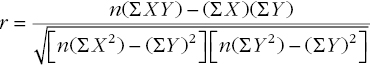
where:

• n = number of observations
• ∑ X = the X variable summed
• ∑Y = the Y variable summed
• ∑ X² = the X variable squared and the squares summed
• (∑ X) ² = the X variable summed, and the sum squared summed
• ∑Y² = the Y variable squared and the squares summed
• (∑Y )² = the Y variable summed, and the sum squared summed

The correlation coefficient is the covariance between two variables divided by the standard deviations of each variable. Standard deviations are always positive, so whether or not the correlation coefficient is positive or negative depends on the covariance.

The correlation coefficient can take on values between –1 and +1. A perfect negative correlation exists when there is a one‐to‐one negative relationship between two variables. Here the correlation coefficient is –1. (See Exhibit 2.1a.) The opposite is the case when there is a perfect one‐to‐one positive relationship between two variables, giving a correlation coefficient of +1. (See Exhibit 2.1b.) If there is absolutely no relationship between two variables, then the correlation coefficient equals 0. (See Exhibit 2.1c.)

In the real world, however, such perfect relationships rarely exist. That is, when there is some relationship between two variables, it will show up in correlation coefficient values between –1 and +1. The closer the coefficient is to +1, the more positive the relationship. In other words, when one variable increases, the other tends to increase as well. (See Exhibit 2.2a.) The closer the correlation coefficient is to –1, the more inverse the relationship. That is, when one variable increases, the other decreases. (See Exhibit 2.2b.)

When we graph the variables and then compute the correlation coefficient, it makes no difference which variable is on the Y axis versus the X axis. The correlation coefficient also does not depend on the specific units of the variables being considered.¹⁰

Correlation Scale

The degree of association between two variables can be put into perspective through the use of a standard correlation scale. This is a mapping of the range of values for the correlation coefficient where the various values are represented as being indicative of the strength of association, be it positive or negative. This mapping technique is useful because it translates the strength of the association into verbal terms that may be easier to understand.¹¹ Correlations greater than 0.5 are considered to be higher than moderate (see Exhibit 2.3).

In addition to the correlation coefficient, economists also express the strength of the association in terms of the coefficient of determination, which is simply the squared value of the correlation coefficient. This measure, r2, shows how much of the variation in one variable can be explained by variation in the associated variables.

One of the advantages of using the correlation coefficient is that it provides a numerical measure of the degree of association rather than simply saying that there is a good association between the variables in question. For example, the expert may be trying to examine the relationship between the sales of a company and certain deterministic factors, such as macroeconomic aggregates like national manufacturing shipments and industrial production. The economist may know that when the economy is expanding, as reflected by upward movements in these macroeconomic aggregates, a company’s sales are expected to increase. The expert may also testify that such a covarying pattern is observable in the data. However, the strength of this testimony may be bolstered by mathematically measuring this association and stating that the correlation coefficient between the company’s sales and total U.S. manufacturing shipments is 0.87, while the coefficient of determination is 0.76. The latter measure means that 76% of the variation in the company’s sales is explained by variation in manufacturing shipments, an indicator used to measure the broad macroeconomic influence of the economy as a whole.

It is important to remember that finding a relatively high correlation coefficient does not prove causality. A high positive or negative correlation coefficient tells us there is a high direct or indirect degree of association between two different series of data, which, in turn, implies that changes in one of the series may cause changes in the other. In our example of the manufacturer, an increase in demand from an expanding economy, as reflected by growth in national manufacturing shipments and increased industrial production, may increase the demand for a company’s product, which, under normal circumstances, would cause the company’s sales to rise. It could be the case, however, that the plaintiff’s sales have fallen and the expected increase failed to materialize. If all other factors can be ruled out, this economic analysis may lend credence to the claim that the actions of the defendant caused the sales of the plaintiff to decline.

Even a high correlation could simply be spurious – without any causality. For example, there is a high correlation between the number of firemen at fires and the severity of fires. This correlation is spurious; one cannot conclude that it is the number of firemen that is causing the severity of the fire. However, a high correlation coefficient can provide a strong suspicion of causality. Even without establishing causality among the associated variables, it may be useful to show that these variables have tended to move together in the past and that something has since caused this association to cease.

Strictly speaking, a correlation of 0 does not necessary mean that there really is no relationship between X and Y. A zero correlation coefficient may mean there is no linear relationship between the variables, but it does not rule out a nonlinear relationship between the same variables. Such a relationship is depicted in Exhibit 2.4, which is the product of a quadratic functional relationship between X and Y.

In economic research, economists sometimes employ econometric tools to analyze causality. Econometrics is the field of economics that applies statistical analysis to economic issues. Within econometrics there is a subfield called time series analysis that investigates causality.¹² However, although these techniques are sometimes used in econometric research, they are not used as often in commercial damages analysis. Other, more basic methods are usually employed. These include the aforementioned correlation analysis as well as graphical analysis in which plots of relevant variables are graphically depicted. For example, Exhibit 2.5 shows a graph of a hypothetical national company’s sales and U.S. retail sales. Such graphs are sometimes referred to as scatter diagrams.

The expert may find that giving the jury the opportunity to visually inspect a plot of the observations over time may reinforce the contention that there is a causal relationship. This is based on the belief that a “picture is worth a thousand words.” In a courtroom, where demonstrative evidence helps win cases, such exhibits can be quite useful. Exhibit 2.5 shows a joint plot of the dependent variable (i.e. the plaintiff’s sales) and a possible causal variable. In cases of a historical business interruption, the graph can be extended beyond the interruption date at trial to help show what sales of the plaintiff would have been absent the interruption. This extension of the “but‐for” stream of plaintiff’s revenues can be constructed using regression analysis. However, putting the correlation analysis together with forecasting techniques allows one to see what happens if the historical relationship that was measured using the correlation coefficient is extrapolated over the loss period.

In conclusion, it is important to note that correlation analysis and graphical demonstration can be very useful but not necessarily conclusive. They can be an important first step in the analytical process. If the results are promising, this may yield a need to continue the analysis further.

Economists and Other Damage Experts: Role of Causality

One of the advantages of using an economist to address causality, rather than using another type of damages expert, is that the economist has training in and regularly uses statistical analysis in his or her work. Statistical and econometric analysis are normal components of the economist’s toolbox. Ignoring causality may be a fatal flaw in the damages presentation. It is pointless to measure damages if they cannot be linked to the actions of the defendant. This issue, and the selection of the correct expert, was clearly demonstrated in Graphic Directions, Inc. v. Robert L. Bush, in which an accountant testified on damages but did not analyze the causal link between the actions of the defendant and the damages.¹⁵ The Court of Appeals of Colorado rejected the damages argument involving a lost customer’s analysis because it did not address this important issue:

Additionally, it is axiomatic that before damages for lost profits may be awarded, one who seeks them must establish that the damages are traceable to and are the direct result of the wrong to be redressed. (citation omitted) GDI’s accountant testified that he did not have an opinion as to whether the losses were caused by Bush and Dickinson’s conduct and stated that he had not related calculation of lost net taxable profits to the lost customers. Nor is there evidence establishing a causal link between all of the lost sales and Bush and Dickinson’s solicitation of customers. At least four of the “lost” customers continued to do business with GDI, and GDI presented no evidence that eight other lost customers did any business with Concepts 3.

Based upon our review of the evidence, we conclude that GDI did not present substantial evidence from which the jury could compute its loss of net profits.

Closed, Open, or Infinite Loss Periods

The loss period is characterized as closed, open, or infinite.¹⁸ In a closed business interruption, the loss period has ended and actual sales, both before and after the interruption, are available. Such a loss period is depicted in Exhibit 2.7. The graph shows that not only has the sales decline ended, the postinterruption revenues have increased beyond the preinterruption level of R1. At time t1, the revenues are consistent with the level that would be forecasted (R2) if we were to extrapolate a simple linear trend from the downturn point.

The loss period is “open” when the losses continue into the future. It can be seen in Exhibit 2.8 that the forecasted revenues are continually above the actual postinterruption revenues and that, although the plaintiff surpasses the preinterruption revenue level of R1, it never returns to its previous growth path. As a result, the plaintiff is continually below where it would have been had it not been for the interruption. An examination of Exhibit 2.8 shows that the firm is growing at the same rate as it did prior to the interruption but that it has “lost ground” during the interruption period. Growth in the postinterruption period at the same rate as preinterruption will never be sufficient to offset the downturn that occurred in the interruption period. Only a higher postinterruption rate of revenue growth would be sufficient to offset the effects of the downturn.

It is important for the reader to bear in mind, however, that these examples are simplistic and feature constant pre‐ and postinterruption growth, so that convenient conclusions, such as full recovery (in Exhibit 2.7) or the inability to ever reach full recovery (in Exhibit 2.8), can be easily attained. In the real world, however, revenues do not behave so conveniently. In such cases, the expert may have to conduct a more sophisticated analysis to determine the actual loss period.

Case of Postinterruption Growth Exceeding Preinterruption Growth

Is it possible for a plaintiff to recover damages if its growth after the business interruption exceeded the preinterruption growth? Just as in the case of a new or unestablished business (see Chapter 5), the analytical and evidentiary burdens of proving such damages beyond a reasonable doubt are greater than when there is dramatic negative growth after the interruption date. However, a plaintiff could indeed be damaged by the fact that it was not able to realize a higher‐than‐actual growth due to the actions of a defendant.

An example of how difficult this is to prove occurred in Bendix Corp. v. Balax, Inc. The defendant‐counterclaimant argued that its growth was less than what it would have enjoyed had it not had to incur the financial pressures brought on by the plaintiff’s patent infringement suit.¹⁹ The defendant’s case was made difficult by the fact that its revenues grew from 8% to 26% over this time period. The defendant argued that its growth would have been even higher. Its president testified that their business was only 60% of what it would have been, and its sales manager said it was only half as large. However, the defendant‐counterclaimant’s proofs – in the form of testimony from members of its management, were unconvincing to the court.

In commenting on the fact that Balax’s revenues increased after the actions of the defendant, the U.S. Court of Appeals for the Seventh Circuit stated:

In the ordinary situation of proving damages allegedly caused as a result of certain action of another, the injured person or corporation shows how its sales declined during the pertinent period but even that is not deemed sufficiently probative. . . . Here, where Balax’s revenues increased very substantially, the evidence of damages consists of (1) VanVleet’s testimony that he thinks that “one of the reasons for Balax’s Detroit representative discontinuing representing Balax was because a Ford Motor Company plant to which he hoped to sell tapes had learned of the infringement suit”; (2) VanVleet’s testimony that “I believe that our business amounted to something like 60% of what it would have amounted to had this action not been brought” and (3) Balax’s sales manager’s testimony that but for the lawsuit sales would be “I would say at least twice as much as we are currently selling.” …

In other words Balax’s business has steadily increased and would have increased more if it had carried cutting tapes, which it does not, through no reason proved to be attributable to the plaintiff.

Disaggregating Revenues by Product Line to Prove Causality

When the defendant’s actions cause a loss in profits for one of a business’s product lines or business segments, it is necessary to disaggregate total revenues and examine the trends in the revenues of the relevant product line or business segment separately. In cases where total revenues for the entire business have increased after the interruption, the defendant may want to examine only the trend in total revenues and thus argue that the plaintiff was not hurt. However, on a disaggregated basis, the plaintiff may be able to show that the product line or business segment’s revenues fell after the interruption.

An example in which the plaintiff made just such a convincing demonstration occurred in Pierce v. Ramsey Winch Co.²⁰ A terminated distributor brought suit against the manufacturer and other distributors. The plaintiff did a standard loss computation in which he projected “but for” revenues, deducted revenues from sales of substitute products, and applied a profit factor to the lost incremental revenues. The defendant argued that the plaintiff could not have experienced a loss since its posttermination gross profits were higher than before. The plaintiff responded that these elevated gross profits came from other goods it sold – truck beds and trailers – not from the winches that were the subject of this litigation. The plaintiff was able to segregate its total revenues and profits, which, when combined with other segments of the business, masked its true losses. The relevant trend was the trend of the product at issue – winches that the manufacturer would have sold to the plaintiff – not in the total revenues and gross profits from the sale of other products unrelated to the case.

The U.S. Court of Appeals for the Fifth Circuit recognized the problems of proving damages when revenues increase after a business interruption, but it also recognized that there are circumstances when damages exist even when revenues and profits have increased.

Pierce Sales, however, cannot show declining sales. As noted Pierce Sales’s gross profits have risen sharply since termination. For this reason Ramsey’s argument that Pierce Sales was not in fact injured by termination indeed has surface appeal.

Improvement in a distributor’s business following termination, it seems to us necessarily flows from (1) a diversion of the resources that were previously devoted to selling products that were supplied by the defendant; (2) successes in an aspect of the business unrelated to the expenditure of resources freed up by the termination; or (3) a combination of these two sources.

If the distributor’s successes flow from the utilization of resources other than those previously devoted to selling the defendant’s products, post‐termination profits would have no bearing on the fact of damage flowing from termination. If the evidence shows, on the other hand, that post‐termination profits exceed pretermination profits, and that they are attributable to the use of resources diverted because of termination to other endeavors, it would seem at least possible that post‐termination endeavors are more profitable for plaintiff than operation of the defendant’s distributorship. We do not think, however, that a plaintiff is necessarily precluded from showing fact of damage in this latter situation. He may demonstrate fact of damage by showing that (1) he lost sales or revenues during the lag period between termination and completion of his efforts to divert resources to substitute endeavors and (2) although substitute endeavors proved more profitable than distribution of defendant’s products did immediately prior to termination, to a level sufficient to earn him greater profits than his substitute endeavors did. He cannot, however, make this showing through speculation or through reliance on unfounded assumptions.

Pierce v. Ramsey Winch Co. is instructive in that it shows that analyzing and graphing total revenues may not capture the relevant trends if only a portion of the business is affected by the defendant’s actions. If this occurs, it is necessary to first disaggregate the revenues by business segment and graph these trends separately. It may also be wise to do a separate statistical analysis of the relationship between the revenues of the various segments and their causal factors.

Disaggregating Revenues to Show Spillover Losses

A defendant’s actions that were directed at one part of the plaintiff’s business may have “spillover” effects onto other parts of the plaintiff’s business. In cases like this, it may not be possible to credibly prove damages by merely disaggregating revenues. It may be necessary to disaggregate costs as well. This is sometimes difficult, particularly when inputs are used for a variety of products. An example in which a plaintiff claimed losses on related products resulting from a cutoff of beer supply is found in Cooper Liquor Inc. v. Adolph Coors Co. The plaintiff claimed that beer sales were a loss leader and were used to bring in customers who would buy other products that generated positive profits. The court rejected the plaintiff’s loss analysis because it was based on gross bank deposits with no product by‐product breakdown.²¹ The lesson from this case is that when claiming interrelated spillover effects, a product‐by‐product revenue analysis must demonstrate these effects. This means constructing a table that analyzes the trends not only in historical total revenues but also in disaggregated components.

Long‐term Contracts

For long‐term contracts, some courts have been reluctant to award damages for the full length of the loss period due to concerns over the degree of certainty associated with long‐term projections. The courts have correctly concluded that the farther into the future one forecasts, the greater the uncertainty surrounding the forecast. In a number of instances, courts have chosen to award damages for periods that are significantly shorter than the actual number of remaining years on the contract. In Palmer v. Connecticut Railway & Lighting Co., for example, the court awarded damages for only 8 years, even though the remaining time on the contract was 969 years and the plaintiff itself conceded that it could not project damages beyond 40 years due to the uncertainty of such a projection.²³ In another example of the court’s simply truncating the remaining years of a contract, the court in Sandler v. Lawn‐a‐Mat Chemical & Equipment Corp. allowed damages for only 3 years although the contract had a term of 50 years with an option to renew for another 50 years.²⁴

One issue that the court has not addressed is the implicit estimate of no losses that this truncation process places on the remaining years of contract. By terminating the losses at a certain date, the court is substituting its own estimate of $0 for losses after the truncation period. The court’s position that only damages that can be projected with reasonable certainty are allowed, however, is affirmed in these and other decisions. The courts are simply saying that there may be losses, but that at some point in the future such losses may not be measurable with reasonable certainty. In addition, after some passage of time, it becomes more reasonable that the plaintiff would be able to pursue other mitigating activities.

A. Macroeconomic Analysis

Using a top‐down due diligence process, this methodology first examines the overall macroeconomic environment within which the alleged loss took place. This examination considers the condition of the overall economy as measured by several relevant macroeconomic aggregates. The performance of the macroeconomy is then compared to the performance of the plaintiff before and after the event(s) in question. The expert will determine, based on the analysis of the company’s historical performance compared to macroeconomic aggregates, what role such variables play in determining the success of the plaintiff. In doing so, the expert will also consider the role that the cyclical variation in the economy has played in the company’s performance and the alleged losses.

B. Industry Analysis

An analysis of the plaintiff’s industry provides valuable information about the performance and profitability of the business area within which the plaintiff operates. This, in turn, can give clues as to how the plaintiff should have performed and what level of profits it should have derived absent the alleged wrongdoing. It allows the expert to see if the trends that are at issue in the litigation, such as the plaintiff’s losses, are specific to it or are part of a wider industry phenomenon that has nothing to do with the actions of the defendant. In order to do this, though, the expert needs to analyze the industry and to determine to what extent that plaintiff is similar to its industry peers. In many cases, there are subcategories within an industry, and the expert may end up comparing the plaintiff with a subgroup as opposed to a broader collection of companies that make up the industry.

Several different data sources are used to measure this industry performance. They tend to vary in quality across industries. Some industries gather abundant and reliable data; others have limited data available and they may not be collected in a reliable manner. This area needs to be explored by the expert. Industry analysis is discussed in Chapter 4.

C. Firm‐specific Analysis

Having established the macroeconomic, regional, and industry environment within which the firm operates, the next step in the top‐down process is to analyze the performance of the firm itself. This includes an analysis of the firm’s historical and current performance as measured by several variables (revenue growth and a number of profitability measures). Depending on the type of case, this firm‐specific analysis may include an analysis of the firm’s financial statements. Such analysis may differ depending on the reliability of the data contained in the plaintiff’s financial statements. Such statements may be audited or merely compiled. Nonetheless, the analysis of these financial statements may employ the standard tools of corporate finance, such as financial ratio analysis. It also may involve analysis of the financial trends of the business, such as those apparent in its historical revenues and profits. In addition, this analysis may be considered in light of the aforementioned economic and industry data.

D. Measurement of Lost Profits

Having analyzed the performance of the plaintiff in relation to the macroeconomic, regional, and industry economic environments, the expert can begin the actual loss measurement process. This typically involves a two‐part process whereby revenues first are forecasted and then a relevant profit margin is applied to the forecasted revenues. The economic, industry, and firm‐specific analyses may all be considered when determining both the base and the growth rates to be used in the forecasting process. Once the revenues and lost revenues are estimated, the lost profits on these revenues need to be measured. To do this, a profit margin has to be established. In order to derive the appropriate profit margin, a cost analysis must be conducted to determine the incremental costs associated with the lost incremental revenues. This loss measurement process combines the forecasting skills of an economist with the costs measurement abilities of either an economist or an accountant to derive lost profits.

E. Adjustment for the Time Value of Money

The estimated loss measures have to be converted to present value terms so that both historical and future loss amounts are brought to terms that are consistent with the date of the analysis or the trial date. A prejudgment return may be applied to pretrial amounts to make them current. Whether this is done, and what rate is used, depends on the relevant law. Similarly, the projected future losses need to be brought to present value through the use of a relevant discount rate. This rate should reflect the perceived risk of the lost earnings stream.

References

- Aetna Life and Casualty Co. v. Little, 384 So. 2d 213 (Fla. App. 1980).
- Agresti, Alan. Statistical Methods for the Social Sciences, 5th ed. Boston: Pearson, 2018.
- Bendix Corp. v. Balax, Inc ., 471 F2d 149 (7th Cir. 1972).
- Bonanomi, Laura, Patrick A. Gaughan, and Larry Taylor. “A Statistical Methodology for Measuring Lost Profits Resulting from a Loss of Customers.” Journal of Forensic Economics 11 (2) (1998): 103–113.
- City of Greenville v. W.R. Grace & Co ., 640 F. Supp. 559 (D.S.C. 1986).
- Conway, Dolores A., and Harry V. Roberts. “Regression Analysis in Employment Discrimination Cases,” in Statistics and the Law, Morris H. DeGroot, Stephen E. Feinberg, and Joseph B. Kahane, eds. New York: John Wiley & Sons, 1986.
- Cooper Liquor Inc. v. Adolph Coors Co ., 509 F2d 758 (5th Cir.) Denying petition for rehearing, 506 F2d 934 (5th Cir. 1975).
- Custom Automated Machinery v. Penda Corp ., 537 F. Supp. 77 (N.D. Ill. 1982).
- Dunn, Robert L. Expert Witness: Law & Practice, vol. 1. Westport, CT: Lawpress, 1997.
- Dunn, Robert L. Recovery of Damages for Lost Profits, 6th ed. Westport, CT: Lawpress, 2005.
- Gaughan, Patrick A. “An Application of Exposure Measuring Techniques to Litigation Economics,” paper presented at the Eastern Economics Association Annual Meetings, 1988.
- Granger, C.W.J. “Investigating Causal Relations by Econometric Models and Cross Spectral Models.” Econometrica 37 (January 1969).
- Graphic Directions, Inc. v. Robert L. Bush, 862 P. 2d 1020 (Colo. App. 1993).
- John J. Terrell v. Household Goods Carriers’ Bureau, 494 F. 2d 16 (Fifth Circuit, 1974).
- Katskee v. Nevada Bob’s Golf, 472 N.W. 2d 372 (November 1991).
- Maddala, G.S. Introduction to Econometrics. New York: Macmillan, 1988.
- Mason, Robert D., and Douglas A. Lind. Statistical Techniques in Business and Economics, 10th ed. New York: Irwin/McGraw‐Hill, 1999.
- McGlinchy v. Shell Chemical Co ., 845 F2d 802 (9th Cir. 1988).
- Palmer v. Connecticut Railway & Lighting Co ., 311 U.S. 544 (1941).
- Parsons, Leonard, and Randall L. Schultz. Marketing Models and Econometric Research. New York: North Holland Publishing, 1978.
- Pierce v. Ramsey Winch Co ., 753 F2d 416 (5th Cir. 1985).
- P.R.N. of Denver v. A.J. Gallagher & Co ., 521 So 2d 1001 (Fla. Dist. Ct. App. 1988).
- Sandler v. Lawn‐a‐Mat Chemical & Equipment Corp ., 141 N.J. Super. 437, 358. A. 2d 805 (1976).
- Target Market Publishing, Inc. v. ADVO, Inc ., 136 F3d 1139; 1998 U.S. App. Lexis 2412.
- Trout, Robert R. “Duration of Employment in Wrongful Termination Cases.” Journal of Forensic Economics 8 (2) (1995): 167–177.
- Trout, Robert R., and Carroll B. Foster. “Business Interruption Losses,” in Litigation Economics, Patrick A. Gaughan and Robert Thornton, eds. Greenwich, CT: JAI Press, 1993.
- Vuyanich v. Republic National Bank of Dallas (D.C. Tex. 1980).
Notes
- 1 Robert L. Dunn, Expert Witness: Law & Practice (Westport, CT: Lawpress, 1997), vol. 1, p. 160.
- 2 Target Market Publishing, Inc. v. ADVO, Inc., 136 F3d 1139; 1998 U.S. App. Lexis 2412.
- 3 Katskee v. Nevada Bob's Golf, 472 N.W. 2d 372 (November 1991).
- 4 P.R.N. of Denver v. A.J. Gallagher & Co., 521 So 2d 1001 (Fla. Dist. Ct. App. 1988).
- 5 Pierce v. Ramsey Winch Co., 753 F. 2d 416 (5th Cir. 1985).
- 6 McGlinchy v. Shell Chemical Co., 845 F2d 802 (9th Cir. 1988).
- 7 Dolores A. Conway and Harry V. Roberts, “Regression Analysis in Employment Discrimination Cases,” in Statistics and the Law, Morris H. DeGroot, Stephen E. Feinberg, and Joseph B. Kahane, eds. (New York: John Wiley & Sons, 1986), pp. 107–168.
- 8 Vuyanich v. Republic National Bank of Dallas (D.C. Tex. 1980).
- 9 John J. Terrell v. Household Goods Carriers' Bureau, 494 F. 2d 16 (Fifth Circuit, 1974).
- 10 Alan Agresti, Statistical Methods for the Social Sciences, 5th ed. (Boston: Pearson, 2018), p. 262.
- 11 Robert D. Mason and Douglas A. Lind, Statistical Techniques in Business and Economics, 10th ed. (New York: Irwin/McGraw Hill, 1999).
- 12 The statistical technique in the econometric field of time series analysis called Granger causality, named after Nobel Prize – winning economist Clive Granger, can be used in a regression of a dependent variable time series {yt} against an independent variable time series {xt}. One can conclude that series {xt} fails to Granger cause {yt} if a regression of yt on lagged xt's reveals that the coefficients of the xt's are zero. The validity of the Granger test comes from the basic premise that the future cannot cause the past. “If event A occurs after event B, we know that A cannot cause B. At the same time, if event A occurs before B, it does not necessarily imply that A causes B.” It is important to bear in mind that Granger causality is not causality in the legal sense. For further discussion of this technique, see C.W.J. Granger, “Investigating Causal Relations by Econometric Models and Cross Spectral Models,” Econometrica 37 (January 1969): 24–36, and G.S. Maddala, Introduction to Econometrics (New York: Macmillan, 1988).
- 13 Laura Bonanomi, Patrick A. Gaughan, and Larry Taylor, “A Statistical Methodology for Measuring Lost Profits Resulting from a Loss of Customers,” Journal of Forensic Economics 11(2) (1998): 103–113.
- 14 Robert R. Trout, “Duration of Employment in Wrongful Termination Cases,” Journal of Forensic Economics 8(2) (1995): 167–177.
- 15 Graphic Directions, Inc. v. Robert L. Bush, 862 P. 2d 1020 (Colo. App. 1993).
- 16 Patrick A. Gaughan, “An Application of Exposure Measuring Techniques to Litigation Economics,” paper presented at the Eastern Economics Association Annual Meetings, 1988.
- 17 Leonard Parsons and Randall L. Schultz, Marketing Models and Econometric Research (New York: North Holland Publishing, 1978), pp. 82–85.
- 18 This categorization of loss periods is derived from Robert R. Trout and Carroll B. Foster, “Business Interruption Losses,” in Litigation Economics, Patrick A. Gaughan and Robert Thornton, eds. (Greenwich, CT: JAI Press, 1993).
- 19 Bendix Corp. v. Balax, Inc., 471 F2d 149 (7th Cir. 1972).
- 20 Pierce v. Ramsey Winch Co., 753 F2d 416 (5th Cir. 1985).
- 21 Cooper Liquor, Inc. v. Adolph Coors Co., 509 F2d 758 (5th Cir.) Denying petition for rehearing, 506 F2d 934 (5th Cir. 1975).
- 22 Aetna Life and Casualty Co. v. Little, 384 So. 2d 213 (Fla. App. 1980).
- 23 Palmer v. Connecticut Railway & Lighting Co., 311 U.S. 544 (1941).
- 24 Sandler v. Lawn-a-Mat Chemical & Equipment Corp., 141 N.J. Super. 437, 358. A.2d 805 (1976).