CHAPTER 10
Securities‐Related Damages
In the wake of the booming stock market of the 1990s and its subsequent collapse, a large volume of lawsuits ensued. Some were motivated by large‐scale scandals, such as Enron, WorldCom, and Global Crossing. Others were caused by the large losses some investors incurred in their portfolios. In 2003, the industry was experiencing a “tidal wave” of arbitration cases.1 Such a volume of securities lawsuits expands the need for finance experts to analyze allegations of damages. The market underwent a prodigious collapse in 2020 after a decade long bull market. It is not clear at this time to what extent this coronavirus‐related collapse may also result in a volume of securities lawsuits.
Key Securities Laws
The two main securities laws in the United States are the Securities Act of 1933 and the Securities Exchange Act of 1934. Conceived during the Great Depression and after the stock market crash of October 1929, these laws were designed to regulate securities markets through mandated disclosure of more accurate, verified financial information and through the prevention of improper activities.
Securities Act of 1933
This law states registration and distribution requirements for public issuers of securities. Companies that issue securities to the public are required to disclose accurate information in their filings and other communications to shareholders. The dissemination of information known to be inaccurate can give rise to a cause of actions by investors who were adversely affected through their reliance on this information. In the wake of scandals such as Enron, the accuracy and adequacy of disclosed financial data have become a major issue.2 Fiduciaries and professionals, such as accountants, may be held liable for the inaccurate information. However, defendants in such actions may try to assert defenses such as stating that investors were aware of the inaccurate information or that they (the defendants) did not know the information was false. Such suits require that experts analyze the damages arising from cases in which investors lost some or all of their investment as a result of inaccurate or false information.
Securities Exchange Act of 1934
This law regulates the trading of securities in the secondary market following their issuance in the primary market. This law requires companies to regularly file statements containing financial and other relevant information with the Securities and Exchange Commission (SEC) – an entity created by this law. The Securities Exchange Act has been amended several times since 1934. Its current form makes illegal such practices as insider trading and market manipulation. Examples of market manipulations include what is known as pump‐and‐dump transactions, whereby individuals or firms engage in deceptive trades and disseminate inaccurate information to try to push up the price of a security, only to sell it to other investors who are not aware that the market interest and rising prices were contrived. Such manipulations have plagued the penny stock market – unscrupulous investment bankers can more easily manipulate the market for lesser‐known publicly held companies.
Rule 10b‐5 of this law prohibits a variety of fraudulent practices, such as disseminating untrue or misleading information or simply engaging in what this section of the law considers fraudulent securities activities. Violations of this part of the law are often referred to as 10b‐5 violations.
Private Securities Litigation Reform Act of 1995
The Private Securities Litigation Reform Act of 1995 (PSLRA) was the first major revision of the above‐mentioned securities laws. It was designed in part to curb abusive litigation practices by private plaintiffs – especially those related to class actions under Rule 10b‐5. Securities lawsuits can be divided into two categories: public and private lawsuits. Public lawsuits are those pursued by a governmental entity, such as the SEC. However, individual plaintiffs can pursue their own securities lawsuits. PSLRA was designed to curb abuses in private securities lawsuits. PSLRA imposed new requirements on such lawsuits and had an important impact on class action suits. Although this law imposed new regulations on class actions, some of the largest class actions occurred after the law’s passage.
The typical class action follows a drop in an issuing company’s stock price. Plaintiffs file suit alleging that the company made overly optimistic disclosures in light of the information that led to the fall in the stock price. An example of the extreme abuses that the act sought to correct is the lawsuit against Philip Morris that followed the “Marlboro Friday” announcement on the morning of April 2, 1993: Philip Morris announced a $0.41 drop in the price of a pack of Marlboro cigarettes.3 Just five hours later, a class action suit was filed, followed by four more suits later in the day and five more the following Monday.4 The courts found the poor quality of the complaints laughable. Plaintiff’s counsel apparently overwrote files from a prior case featuring a toy company, discussing Philip Morris’s future success in the toy industry. Clearly, the speed with which the cases were filed prevented any meaningful research into the grounds for the fraud claims.
Among the regulations this law added is the requirement that settlements be disclosed to the class. Plaintiffs in class actions are required to demonstrate that they did not purchase the securities at the direction of plaintiff’s counsel, that they reviewed and authorized the complaint, and that they disclosed all of their trades of the security in question as well as their activity in other securities lawsuits. In part, the law was designed to try to curb law firms that were pursuing such suits to receive “fee‐mail” in settlements and employing professional plaintiffs who purchase the shares with the intention of suing. Under PSLRA, a defendant can object to the selection of a lead plaintiff if it believes that he or she is a professional plaintiff. The law also governed the use of forward‐looking statements. Such statements need to be clearly labeled as forward‐looking, and they must include appropriate cautionary language.
From a damages perspective, this law requires the plaintiff to demonstrate that the actions of the defendant directly caused the plaintiff’s damages. For example, in cases where a plaintiff alleges that the defendants disseminated financial statements featuring inflated profits, he or she must demonstrate that the stock moved in a manner that adversely affected him or her owing to this false information (rather than market movements). PSLRA also imposed a strong scienter requirement where the plaintiff must be prepared to demonstrate that the defendant acted with a particular state of mind that was bent on fraudulent intent.
In addition to the preceding provisions, this law also sets forth parameters within which damages may be computed in fraud‐on‐the‐market claims. These parameters included a cap on damages. This cap limits a plaintiff’s recovery to the difference between the sale price of a security and its average price over a 90‐day period after the disclosure that is at issue in the lawsuit. The use of such an average limits the short‐term impact of any possible overreaction to the news.
Congress, in passing PSLRA over President Clinton’s veto, attempted to accomplish four goals:
- Reduce the number of lawsuits that occur after a sharp drop in a company’s stock price (called strike suits) but where the company did not engage in any wrongdoing.
- Reduce the number of suits aimed at “deep‐pocketed” defendants who may be easily able to settle a suit for an amount that would be relatively small to them but significant compensation to the plaintiff and its counsel.
- Reduce the use of aggressive discovery practices that amount to burdensome fishing expeditions.
- Reduce the overly aggressive and unethical practices of some members of the plaintiff’s bar.5
Various studies have attempted to measure the impact of PSLRA on the markets. Some initial studies found that the Act had a wealth increasing effect on the value of equities.6 Choi, Nelson, and Pritchard found that while there was not enough evidence to conclude that PSLRA led to a reduced incidence of claims that end up being settled for nuisance value, they did find that non‐nuisance claims were less likely to be filed after the passage of the law. Thus they concluded that the law had a measurable screening effect.7
A study by Johnson et al found that PSLRA resulted in a shift away from lawsuits based upon forward looking earnings disclosures. They also found that after PSLRA there was a greater correlation between securities litigation and earnings restatements as well as abnormal selling by insiders.(*)
Sarbanes‐Oxley Act of 2002
Although the Securities Litigation Reform Act of 1995 placed needed curbs on abusive plaintiffs and their law firms and thereby aided potential defendants, it imposed greater requirements on potential defendants. Financial statements that are filed with the SEC must now be certified by the chief executive and chief financial officers of the issuer, who must clearly state that the statements do not contain any information known to be false. The law applies to both quarterly and annual financial statements and the filings that contain them – 10Qs and 10Ks, respectively. The officers who sign such certifications are responsible for establishing controls that ensure their accuracy. Officers who violate this law are subject to fines that can be as high as $5 million; they also can face imprisonment for up to 20 years. If the financial statements have to be restated due to inaccuracies, the officers may also have their compensation forfeited.
The law also imposes restrictions on accountants who certify such statements. It attempts to eliminate a conflict of interest on the part of accountants who are auditing companies and at the same time profiting from other consulting work for the issuer. The law sets forth a variety of services, including actuarial, valuation, broker/dealer, and investment banking, which auditors are expressly prohibited from providing to their audit clients. Accounting firms may perform nonaudit services, but they must be approved by the audit committee and be disclosed in the periodic reports that are filed.
Trends on Class Action Lawsuits
The number of class actions filings declined in 2009 compared to 2008 as the nation entered the subprime crisis. Thereafter the levels remained somewhat below the levels during the years 2000–2008 (with the exception of 2006 when the numbers were unusually low). However, starting in 2005 the volume of class actions picked up and surged to high levels over the years 2018–2019 when the numbers were more than double what they were in 2008–2014 (see Exhibit 10.1)(*).
Trends in Class Action Settlements
The dollar value of class action settlements has been volatile with no clear trend. Relatively high dollar amounts have been followed by lower values in the next year and vice versa. Naturally, there is a lag between the volume of filings, numbers which were significantly higher over the years 2017–2019, and subsequent settlement values. It is noteworthy that Cornerstone found that the disclosed market capitalization losses in the years 2018 and 2019 were also up sharply.(*) Thus far, these have not translated into higher settlement values but this could be due to the fact that there has not been sufficient research on the causality and timing of filings and settlement values.

EXHIBIT 10.1 Number of class action filings.
Source: Cornerstone research.
Damages in Securities Litigation
Damages can take on different forms in securities litigation. The most common types of damages here are:
- Fraud‐on‐the‐market
- Mergers‐related damages
- Churning and broker portfolio mismanagement

EXHIBIT 10.2 Mean and median estimated damages by year.
Source: Cornerstone research.
Fraud‐on‐the‐Market
The term “fraud‐on‐the‐market” refers to the sale of securities pursuant to some material misrepresentation that investors may have relied on. Some have pointed out that part of the fraud‐on‐the‐market argument relies on a blind trust in the integrity of the market – a potentially higher standard than nonfinancial markets.8 It is an example of a violation of Rule 10b‐5. SEC Rule 10b‐5 proscribes behaviors such as the release of false and misleading information or the failure to release relevant and legally required information to the market. In Basic the court endorsed the presumption that some markets, such as those actively traded with large equity trading volumes on organized exchanges such as the New York Stock Exchange, are efficient. Indeed, Basic, which was rendered in 1988, reflected the large volume of financial research supporting market efficiency that was abundant and prevalent at that time. However, over time more and more research on inefficiencies emerged. Thus, the automatic presumption of efficiency, especially in cases involving companies traded on major exchanges, is no longer automatic but has now become a proposition that can be debated by both parties in a fraud‐on‐the‐market loss analysis.
One of the most common ways a 10b‐5 violation may occur is when an issuer has released financial information that creates an overly optimistic picture of the company’s financial condition. For example, a company may have inflated its profits by releasing inaccurate financial data. This could come from overstated revenues or understated costs. Other examples of a fraud‐on‐the‐market can come from misleading or inaccurate statements about events that affect the stock price. An example is a denial of merger negotiations when such negotiations were actually taking place. This is actually what occurred in the Basic, Inc. v. Levinson case.
Basic, Inc. v. Levinson
One of the most famous cases in this area was Basic, Inc. v. Levinson. In this case, representatives of Basic, Inc. denied in public statements that merger negotiations were ongoing. However, starting in the fall of 1976, representatives of Basic, Inc. had active discussions with Combustion Engineering, Inc. regarding the possibility of a merger. In December 1978, some investors were surprised to learn that Basic, Inc.’s board of directors had approved a merger with Combustion Engineering.
It was argued that had this fact been disclosed, the stock would have traded at a higher price. This is due to the fact that in acquisitions, target shareholders receive a premium above the stock’s price.9 Shareholders who sold their shares, believing that a takeover premium was not forthcoming, may have incurred damages by selling their holdings at a lower sales price. The plaintiffs in this case were one‐time shareholders in Basic, Inc., a manufacturing company whose shares traded on the New York Stock Exchange. They successfully argued that they sold their shares at artificially depressed prices due to the fact that the market was not aware of the impending tender offer from Combustion Engineering.
In Basic, the Supreme Court considered a Sixth Circuit Court of Appeals decision that affirmed the granting of class status to shareholders of Basic, Inc. The district court granted a plaintiff’s motion seeking class certification. The matter ultimately was brought to the U.S. Supreme Court.
BASIC, INC. V. LEVINSON AND MARKET EFFICIENCY
In its plurality opinion, the Basic Court endorsed the efficient markets hypothesis.10 This theory of financial markets considers the speed or efficiency with which financial markets internalize new information into the prices at which securities trade.11 There are three versions of the efficient markets hypothesis: strong form, semi‐strong form, and weak form. In the strong form, all information (both public and private) is internalized in securities prices. The semi‐strong version assumes that the market is efficient with respect to public information only. The weak form focuses on one type of public information – prior trends in security prices – and assumes that the securities prices internalize this particular type of information. In Basic, Inc. v. Levinson, the court endorsed the semi‐strong version of the efficient markets hypothesis. In doing so, it assumed that if information on merger discussions had been given to investors, the market would have incorporated this into the prices of Basic’s stock. The extent to which markets are considered efficient has been one of the most actively researched topics in finance.12 Much of the research literature in this area relies on event studies; they look at the market’s security price reaction to the dissemination of a particular type of information. Later in this chapter we will briefly discuss what some of these research studies show with regard to the efficiency and inefficiency of markets.
In a Basic‐type argument, plaintiffs must prove that their shares traded in an efficient market.13 Therefore, plaintiffs need to prove that the alleged misrepresentation was public and material while also showing that the stock traded in an efficient market. Once those factors are established, then Basic asserts that the plaintiffs are entitled to the presumption that the misrepresentation was internalized into the stock price. Also, as per Basic, the plaintiffs are also entitled to the presumption of reliance. These are strong conclusions and for some time many believed that the court in Basic went too far.
As we have noted, part of the court’s reasoning in Basic, a 1988 case, was a function of the times. The early research, following up on Professor Fama’s seminal article, was generally quite supportive of market efficiency.14 Professor Fama’s early research emphasized the proposition that stock prices may follow a random walk process. He later refined this assertion to contend that stock prices fully reflect all information.15
Following these seminal papers, along with another from Nobel prize winner Paul Samuelson, it seemed that market efficiency was becoming ingrained in finance thought.16 These propositions were supported by a very large volume of empirical research in support of the hypothesis.
That early research, far too voluminous to discuss in detail in this volume, numbers in the hundreds.17 It used event studies to show that events such as public announcements of exchange listings, new product announcements and annual earnings reports, and others could not be used to beat the markets after taking into account factors such as transactions costs. It was such research that the Supreme Court, in its decision in Basic, along with much of the field of academic finance, seemed heavily influenced by. A little later in this chapter we will discuss further some of this research and how it has evolved in the years after Basic.
In a dissenting opinion, Justice White “inherently recognized the potential problems that may result when courts are asked to intermingle legal concepts with economic theories.” This opinion would prove to be quite relevant in the years after the decision, as the research landscape in finance changed with more and more studies punching holes in parts of the efficient markets hypothesis. As we will discuss below, in the years after Basic, courts have clarified what they consider to be an efficient market and its significance.
Market Conditions and Market Efficiency
Market conditions can affect how efficient markets really are. Market makers and arbitragers play important roles in keeping markets efficient. Market makers bring buyers and sellers together. Arbitragers may bring about the law of one price by trying to identify overpriced and underpriced opportunities. When we have very unusual market conditions, such as what occurred during the subprime crisis, market participants may “run away” from the market, leaving it somewhat devoid of these key participants.18 When they are not active in the market, it can use lose its efficiency. Thus, for this reason, and others, market efficiency should not be blindly assumed.
Cammer Factors
One year after the Basic decision, a district court in Cammer v. Bloom provided further clarity to applying the court’s reasoning set forth in Basic with respect to how market efficiency can be determined. In Cammer, a defendant, Coated Sales, Inc., filed for bankruptcy following an announcement of its overstated financials over the prior two years.19 The efficiency of markets became an issue in determining if the markets reflected the false financial information. The defendant’s securities traded in NASDAQ. In reaching its decision the court identified five factors that have come to be known as “Cammer Factors.” They are:
- High weekly trading volume
- A number of market makers and arbitragers
- Analyst coverage
- Ability of the company to file an S‐3 registration statement
- Evidence of a historical empirical relationship between new information and past movements in the company’s stock price.
A high trading volume creates an opportunity for stock prices to possibly better reflect new information. This level of efficiency may be enhanced by market makers who buy and sell the securities of the company. Arbitragers may also trade the securities when they spot inefficiencies. For example, if an arbitrager sees that the stock price is below the value the arbitrager places on the shares, then this investor will see this as a buying opportunity. The opposite would be the case for an overvaluation, which could create a profitable selling opportunity.
The court in Cammer recognized that it could be useful to be able to demonstrate that in the past the stock did respond in an efficient manner to prior announcements of relevant information. This can be done by a statistical analysis that identifies past releases of information and relates that the movements in the company’s stock price – movements that go in the expected direction.
An S‐3 form is the most simplified registration form that public companies file with the SEC in the U.S. To be eligible to file an S‐3 form a company must have been required to report to the SEC for at least 12 months and have filed all their required reports, such as 10Qs, 10Ks, and 8Ks, on a timely basis. There are several other relevant requirements such as having a public float of at least $75 million. Others include the requirement that the company must not have defaulted on any of its debt obligations and must not have missed any dividend payments on its preferred stock. In the Cammer case, Coated Sales had not filed with the SEC for a year and a half, and, therefore, could not file a Schedule S‐3.
A study conducted at NERA tried to ascertain how courts apply Cammer factors. In an analysis of decisions over the period 2002–2011, and the respective factors at play in each case, they found that “in over 98 percent of the cases, the ultimate ruling on efficiency can be predicted by the number of factors that the court found efficient less the number of factors that the court argued against efficiency. When the figure was positive, the court found the security at issue to have traded in an efficient market in all but one instance, while when the figure was zero, the court always found the security to have traded in an inefficient market. Moreover, just limiting the analysis to three Cammer factors (turnover, analysts and market makers) yielded similar results.”20
Other Factors: Krogman Factors
At times courts have considered other factors that might reflect market efficiency. In Krogman v. Sterrit, the U.S. District Court for the Northern District of Texas looked to factors such as market capitalization, bid/ask spreads, and float. Under the Krogman court’s reasoning, companies that have larger market capitalizations may be considered more efficient. The court also viewed companies with more narrow spreads as trading in more efficient markets. Lastly, this court considered that the higher percent of shares that are traded, or floated, in markets, the more efficient the market.
Tests of Market Efficiency
Above we have discussed examples of market inefficiency. Clearly, all markets are not at all times efficient. Markets can vary in the extent to which they are efficient as a function of the specific market, such as New York Stock Exchange as opposed to NASDAQ, as well as the time period at issue. It should be kept in mind that markets can be relatively efficient at times and less efficient at other times. The varying degrees of efficiency are underscored by the award of the 2013 Nobel Prize in economics, which was, ironically, shared by Eugene Fama, of the University of Chicago, who is widely known as the father of the efficient markets hypothesis, and Yale’s Robert Shiller, who is one of the leading researchers on market inefficiencies.
Given that there are three different versions of the efficient markets hypothesis, the research literature in the field of financial economics features abundant tests of each form. For many years this area of financial research served as a research forum for studies by young PhDs seeking tenure and/or promotions in academia.
WEAK FORM MARKET EFFICIENCY
Weak form market efficiency implies that stock prices fully reflect all information on past stock prices. Thus, past stock prices can’t be so predictive of future stock prices that they allow the predictor to beat the market after accounting for trading costs. To test this proposition, researchers perform tests such as autocorrelation tests to see if the coefficient of the relationship between a stock price at time t is statistically significantly related to the same stock’s prior stock prices. If, for example, the coefficients were not only statistically significant but also positive, then this implies a positive trend. If it were negative it would imply the opposite. Much to the consternation of many technical analysts, a large body of the initial research on this topic implied that markets tend to be weak form efficient.
Researchers have also used other tests to determine if a series, such as a series of stock prices over time, are what are referred to as a random walk process. If so, then the best predictor of a stock price at time t (Pt), is Pt − 1. One of the simpler tests, which tries to determine if a series is random, is a run test. Such tests can be applied to coin flips where if two flips in a row come up the same side, such as heads, then a run has started. The run continues until tails comes up.
Other tests of the weak form efficient markets hypothesis are tests of specific trading rules that a technical analysis might apply. There are several such “rules.” One example is the “head and shoulder formation.” If the recommendations suggested by the “rule” continue to apply over time, then the market cannot be efficient as it adapted to such a “rule.” The rule should not be effective once the market adapts to the rule’s initial effectiveness.
While there is abundant research that stock prices tend to be weak form efficient, a number of “troubling” studies have called even weak form efficiency into question. For example, Erenburg et al. analyzed the stock prices of companies that were involved in federal class action lawsuits.21 They found that courts may be too quick to certify class actions and automatically assume that simply because a company trades in an active market with relatively high volume does not automatically mean that the market is efficient. Just the presence of high trading volume does not necessarily ensure market efficiency because inefficiencies could actually attract many traders to a particular security in an effort to benefit from its inefficiencies.22
SEMI‐STRONG FORM MARKET EFFICIENCY
If a company’s stock price fails to establish weak form efficiency, then it cannot establish semi‐strong efficiency. Semi‐strong form efficiency implies that all public information, including prior stock price data, but also all other public information such as earnings reports, new product announcements, and exchange listings are internalized on a timely basis in the stock prices. Just as with tests of weak form market efficiency, initially there were many studies showing how markets were semi‐strong efficient. Many of these focused upon a particular type of event, such as an announcement of new products or being listed on a major exchange, both of which could have an uplifting effect on the company’s stock price. However, if such public news could not be used to achieve returns above what would be expected after market factors and trading costs were taken into account, then that market might be considered semi‐strong efficient.
The initial research was quite supportive of equity markets being semi‐strong efficient. However, over time research on persistent market anomalies began to attract the attention of even some of the most ardent supporters of market efficiency.
For example, studies going back to the 1908s have looked at the market’s reaction to annual or quarterly earnings reports as well as a variety of other types of announcements, such as new products or exchange listings. While many studies support market efficiency, many others challenge some aspect of market efficiency. Several of these challenging studies show that market anomalies may exist in which investors may persistently enjoy extranormal profits based on the utilization of public information. One such example is the “turn‐of‐the‐year effect” or “January anomaly” – it has been shown that trading motivated by tax loss can allow investors to realize above‐normal profits.23 Other oft‐cited market anomalies are the size effect and neglected firm effect in which small firms or companies that are not as closely followed can be a source of above‐normal gains.24
The research on market anomalies and instances of inefficiency does not mean that markets do not tend to be generally efficient. However, the fact that research shows that, at times, inefficiencies may exist, requires that litigants in fraud‐on‐the‐market lawsuits need to explore this issue and not blindly assume efficiency.
STRONG FORM MARKET EFFICIENCY
If markets are strong form efficient, then all information, both public and non public, can’t be used to achieve abnormal returns after transactions costs have been take into account. This version of the efficient markets hypothesis is less relevant to the current discussion as we are considering releases or non releases of information to the public market. Moreover, if markets are not semi‐strong efficient, then they cannot be strong form efficient.
Class Actions and Reliance
Pursuant to Rule 23(b)(3) of the Federal Rules of Civil Procedure, class action certification requires the plaintiffs to show that the facts or questions of law at issue predominate over the issues that are specific and unique to each plaintiff. For fraud‐on‐the‐market class action lawsuits, a key issue is establishing the reliance. Reliance means that the plaintiff must establish that misstatements at issue motivated an investor’s decision to engage in given transactions. It is not enough that the plaintiff establish damages; they must also demonstrate that the damages were the result of the misstatements.
In Basic the Supreme Court created the rebuttable presumption of reliance by all class members in actions involving misstatements of omissions of relevant information related to their purchase or sales of an issuer’s securities. The significance of this is that a plaintiff does not necessarily need to show that he or she actually read or heard the misstatement. Thus, Basic shifts the burden to the defendant to disprove reliance. Without reliance plaintiffs cannot proceed with 10b‐class actions seeking damages against an issuer for misstatements that may have inflated the price of its shares. If the plaintiffs cannot get the class certified, the suit will be much less likely to brought.
Theoretically, reliance could be much more challenging for a class action as opposed to an individual plaintiff lawsuit.25 However, this was clarified by the decision in Stoneridge Invest. Partners v. Scientific‐Atlanta, wherein the court indicated that reliance is presumed when the information at issue is made public.26 That is, the court in Stoneridge assumed that the information would be reflected in the market price of the security. The court concluded that buyers and sellers would naturally take relevant information that is public into account when they buy and sell the security. This is an important issue, as it could allow the trier of the facts to determined damages through one common process for the whole class.27 In other words, if the matter is a class action, the damages the class is seeking must be calculable in a common process.28
Further clarification was provided by the Supreme Court’s 2014 decision in the Halliburton case.29 Halliburton II provided clarity on the issue of determining class certification but also how event studies should be used in determining damages in fraud‐on‐the‐market loss analyses and in class actions in particular.
That case arises out of a lawsuit related to a merger between Halliburton and competitor Dresser Industries. The incestuous nature of the parties was troubling. Halliburton’s CEO was none other than Dick Cheney – perhaps better known as George W. Bush’s vice president – and for his role in the disastrous Iraq war and the many U.S. soldiers and also civilians who died as a result of their stupid decisions.30 Dresser had huge potential asbestos liabilities that the plaintiffs, including the Archbishop of Milwaukee, alleged were not disclosed. The plaintiff sued for damages based upon what they considered insufficient disclosure.
In Halliburton II the Supreme Court accepted the case so as to consider whether to overrule or modify its holding in Basic that was the law for roughly a quarter of a century. In a majority decision, and over the objections of three dissenting judges, the Court in Halliburton did not overrule Basic and its presumption of reliance. However, the Court did open the door to future defendants challenging class actions by showing that there was not a price impact.
In light of Halliburton, the parties may employ financial economists and econometricians to conduct even studies at the class certification stage (and later) which can be used to measure a price impact or to show that lack of one. For defendants this could be done through an econometric showing that a corrective disclosure (offsetting the misleading prior positive information) did not have a negative impact on the stock price. The opposite would be the goal for plaintiffs to try to show the there was a negative impact. A showing of a negative impact implies that the misstatements did indeed cause the price to be inflated. Obviously, this process is not as simple as a showing of the movement of the defendant’s stock price on the relevant day. Econometrician may be employed to statistically filter out other influences such as the movement of the market as well as other relevant factors. In addition, our discussion here is simple and a given case may involve multiple misstatements and possibly also multiple different corrective disclosures.
Disgorgement
In SEC enforcement actions, the defendant, if found guilty, may be required to disgorge the ill‐gotten gains. This precedent was established in the Texas Gulf Sulphur cases in which various employees of Texas Gulf Sulphur purchased stock and call options in the company prior to an announcement of a major mining discovery.31 In these cases, the courts required the defendants to disgorge their profits. The amount to be disgorged can be either the actual profits that the defendant enjoyed or what is referred to as paper profits, defined as the difference between what the defendant paid for the shares and the value for them that the court assesses. This value is determined by relevant stock price data around the time of the event. In the case of positive information on which a defendant traded prior to the release of that information to the public, the paper profits are the difference between the price paid for the shares prior to the public announcement and the full information price. The full information price is determined by judgment based on the time that the market has finished reacting to the new information. Paper profits can thus be different from actual profits. If the illegal trader sells at the full information price, the two might be the same. However, if the trader holds on to the shares and other factors cause the stock price to move to another level, the actual profits will vary and will be determined at time of sale. Assume that the trader holds on to the shares and other factors cause the stock price to fall below the purchase price. If that person sells the shares, he or she may be forced to disgorge positive paper profits when his or her overall trading in the stock actually resulted in losses.
Measuring Damages in Fraud‐on‐the‐Market: Out‐of‐Pocket Damages
The most common method of measuring damages for fraud‐on‐the‐market is an out‐of‐pocket measure of damages.32 This measure draws on the reasoning of Judge Sneed in Green v. Occidental Petroleum Corp.33 Judge Sneed set forth an acceptable way of measuring such damages as the difference between what he called the price line and the value line. The price line reflects the “corporate defendant’s wrongful conduct.” In a case involving inflation of corporate profitability, this would be the stock price that was a function of the exaggerated income. The value line is the stock’s price in the absence of exaggerated prices. This difference is depicted in Exhibit 10.3, where the shaded area shows the magnitude of the damages that investors may have incurred. The two curves, called lines by the court, start off at the same point ti and it is assumed that this is the date when the misrepresentation occurred. At this time, it is assumed that an overly optimistic picture of the company’s performance is portrayed, thus causing the market price (as reflected by the price line) to be above what its true value would be absent the misrepresentation.
EXHIBIT 10.3 Price line versus value line.
The measurement of damages can be divided into two parts:
- Establishment of the loss period. The loss period usually begins with the date when the inaccurate information was released to the market. It usually ends with the date of disclosure.34 If one assumes that markets are very efficient, then the time period narrowly focuses on these two dates. If, however, markets are not assumed to be very efficient, then the loss period becomes less clearly centered on these dates.
The establishment of the loss period may not be very clear‐cut. There is usually not just one improper announcement or material misrepresentation. Rather, there is often a series of such false statements. As a result, the expert must make a judgment as to the correct start of the loss period. This judgment is made more difficult when there is a series of improper statements or misrepresentation; the expert must make a determination of when the inflating effects on the market began. The end of the loss period may also be unclear. It may be the case that the issuer makes a series of statements that address the initial misrepresentation. This could cause the market to correct in a series of steps. However, it could cause the market to overreact by thinking that the misrepresentation was greater than what it actually was.
- Measurement of damages. In this model, the measure of damages is the difference between the price line and the value line multiplied by the number of securities in question. The number of shares is estimated using an analysis that attempts to determine how many shares were actually affected and to eliminate shares in which gains offset losses.35 The major challenge here is to calculate the value line. There are different ways to compute this. One is to arithmetically reconstruct what the stock price should have been during the loss period. This method examines the percent change of various other comparable companies and, in doing so, computes the relative change in the stock prices of these companies. This can be done using basic percentages or by employing regression analysis. More formally, the expert may employ what is known as comparable index approach. It attempts to predict the security’s return using explanatory variables such as the market return and the industry return.
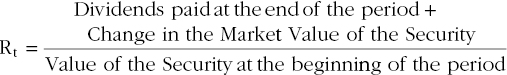
Security and Market Returns
The percentage return of security is defined as the combined effects of the income that is received, such as the dividends from a share of stock, and the price changes of the securities (in the form of capital gains or losses). This percentage return has two components, one of which is the dividend yield. It is the component of the return that is attributable to the dividend income.36 This can be expressed as shown in Equation 10.1.
The other component of the total return is attributable to the security’s price movements; it is called the capital gains return. This is expressed as shown in Equation 10.2.
Both components of a security’s return can be combined to form the percentage return of the security. This is shown in Equation 10.3.
The return on the market can be computed in a similar manner using an accepted market proxy such as the Standard & Poor’s 500 market index. This index uses the market value of the securities to measure the performance of the market.
Comparable Index Approach
The comparable index method uses econometric methods to estimate the relationship between a security’s return and the return of the market and the industry. The relationship is estimated and used to compute the security’s “value.” It is then compared to the security’s actual price. In order to estimate the relationship, historical return data are gathered for the security, the industry, and the market. This period should be one that excludes the alleged fraud so the estimated relationship is not tainted by the events in question. The decision on the proper period to use affects the value of the coefficients α0 … α2 that are estimated. The estimated function is of the form shown in Equation 10.4.
where:
- Rit = the return on security i at time t
- Rmt = the return on the market at time t
- RI t = the return on the industry at time t
The difference between the estimated security value and its actual price is sometimes referred to as the damage ribbon or, simply, inflation. This gap reflects the damages incurred by investors. The relationship between a hypothetical price and the value line is depicted graphically in Exhibit 10.3.
Criticism of the Comparable Index Approach
As with any approach that relies on econometric analysis to estimate the best relationship among variables, there are often disagreements as to whether the expert estimated relationship is the most accurate one. Some contend that the estimate is made more accurate if more explanatory variables, such as more than one index, are added to the model.37
Impact of the Private Securities Litigation Reform Act of 1995 on Damage Computations
The Private Securities Litigation Reform Act of 1995 addressed the way that damages are calculated in Rule 10b‐5 cases. Section 21D (e) of the law states that a damage award shall not exceed the difference between the purchase price of the security and the mean trading price of that security over a 90‐day period. This period begins with the day that the full disclosure, which corrected the misstatement, was made to the market. An exception to this occurs when the security holder sells the shares or repurchases the security prior to the end of this 90‐day period. In this case, the damages cannot exceed the difference between the purchase price and the average of the security’s price at the beginning of the full disclosure period and the price in the subsequent sales transaction.
In Exhibit 10.4, an investor purchases a stock at $30 and the stock price rises to $40. The plaintiffs allege that this rise was due to the false information disseminated by management. When the curative disclosure occurs at time t0, the price falls to $20. Under the parameters of the new law, damages cannot be measured as the difference between the $40 price and the post disclosure price – $20. Exhibit 10.4 shows that over the 90‐day period, t0 + 90, the stock price rebounded to $25. Given this rebounding price rise, the losses are the difference between the purchase price ($30) and this price ($25) for total per‐share damages of $5, not $20.
An exception occurs when the shares are sold during the 90‐day period. In Exhibit 10.5, we assume that the investor bought the stock at the same price – $30. It rose to $40 and later fell to $20 on day t0 after full disclosure. In this example, however, we assume that the stock price falls to $15 per share on t0 + 30 when the investor sold the stock. The average price in the 30‐day period before the investor sold the shares is $17.50. Damages are the difference between the purchase price ($30) and this average price, or $12.50. This example differs from that of Exhibit 10.4 in that not only was the stock sold prior to the 90 days, but the stock price continued to fall in the 30‐day period – although not as sharply as it did on the announcement date. The further decline in the stock price expanded damages, although not by as much as the difference between the purchase price and the eventual sale price of $15. If the price rebounded steadily after t0 as it did in Exhibit 10.4, damages would be less, although still higher than if the stock had been held for the full 90‐day period.
EXHIBIT 10.4 Graphical depiction of stock price cost.
EXHIBIT 10.5 Graphical depiction of stock price damages: stock sold.
Event Study Approach
The event study approach draws on a methodology that has been used extensively in academia for conducting research on the impact of specific events on shareholder returns. In the context of securities litigation, event studies are used to determine if there is a linkage between a specific event, such as a release of false and misleading information to the market, and a change in the value of an issuer’s securities. Events studies have become so ingrained in these types of securities lawsuits that some courts have virtually required them.38
It also can be used to test for the fifth Cammer factor – whether there is a causal relationship between the information disclosures and variation in the price of the securities.
The event study methodology is an application of econometric analysis to securities markets in a manner that allows the analyst to measure the impact of a particular event on the price and return of a security.39 The methodology was developed by Eugene Fama, Franklin Fisher, Michael Jensen, and Richard Roll.40 The model has come to be known as the FFJR model after its developers. Its application has led to the extensive analysis of a variety of events, such as earnings and new product announcements. Abundant research was conducted using this model in the 1970s and 1980s to test the efficiency of securities markets. The event study methodology allows the user to filter out the influence of market forces. The user constructs a regression model that includes market returns as an explanatory variable. In doing so, a security’s return is regressed against the market returns. Equation 10.5 shows the mathematical expression of this relationship in what is known as the market model.
where:
- αi = the intercept term of the market model
- βi = the security’s beta; betas measure security’s sensitivity to market returns
- εit = the model’s deviations at time t
EXHIBIT 10.6 Security’s return versus market’s return.
Exhibit 10.6 shows a graph of a hypothetical security’s return against the market’s return, which is measured as the rate of return of some market index, such as the Standard & Poor’s 500. The exhibit shows that there is a linear relationship between the security’s return and the market’s return. The event study methodology uses this relationship to compute what the security’s return would have been had it not been for the “event” that is the subject of the litigation. However, the event study model computes the relationship between the security’s return and the market’s return prior to the event; it uses the mathematical relationship to forecast the “but for” return of the security. This return can then be compared with the actual post‐event return to measure the excess return of the security. This excess return, in the absence of other explanatory factors, can then be used to measure the magnitude of the loss.
Abnormal Returns of the Event Study Methodology
The market model allows for the separation of the total return of a security into systematic and unsystematic components. The systematic component is the part that can be explained by the market’s return – αi + βi Rmt. According to the market model, the part that cannot be explained by the market’s influences is attributed to firm‐specific effects and is statistically subsumed with the “remainder factor” in the market model’s equation: εit. That is, εit captures the variety of firm‐specific factors including those that are the subject of the litigation – the alleged fraudulently inflated profits of the previous example. The impact of εit can be discerned more readily by arranging Equation 10.5 as follows:
The historical data on Rit and Rmt for the period prior to the event in question, which is taken to be t = 0, are used to econometrically estimate α and β. The values of these two parameters are then used to compute a predicted return, Rit, and its resulting deviation, εʹit, which can then be compared to εit. This represents the deviation of the actual return, inclusive of the effects of the fraudulent behavior, from the predicted return as measured using the market model’s estimated parameters α and β. This discussion is sometimes also expressed through the estimation of abnormal returns where abnormal returns are equal to:
where:
- ARit = abnormal returns
- αʹi = the estimated alpha
- βʹ = the estimate of beta
EXAMPLE OF A ONE‐PERIOD ABNORMAL RETURN
As an example of a one‐period abnormal return, assume that:
The one‐period abnormal return is simply:
The abnormal returns just computed apply to just one period, i, which may be one day. When the event window is longer, then it is necessary to compute the cumulative abnormal returns (CAR). This is a running total of the one‐period abnormal returns for the length of the study period. This is mathematically expressed as:
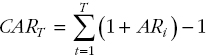
where:
- T = the length of the study window
When we compute CART, we have a measure of the total impact of the event.
Examining the Variation in Abnormal Returns
Once the security’s return has been computed, it may be useful to examine the variability in the return. In analyzing the variation in a security’s return, it is useful to compute the standard deviation of the return. A security’s return does not stay constant; it normally varies. One simplifying assumption that is made is that the variation fits a pattern that would be expected if the return were normally distributed. While not perfect, the assumption of normality is commonly made in event studies.41 The standard deviation of a security’s returns can be computed as shown in Equation 10.9.42
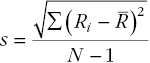
where:
- R = the mean or average return over the sample period
The standard deviation can be used to test the statistical significance of the variation in a return. Using the assumption of a normal distribution, we expect that 68% of the returns will lie within 1 standard deviation of the mean. Of the returns, 95% will lie within 2 standard deviations while 99.7% will be within 3 standard deviations. We can take the standard deviations that we have computed to arrive at what is called a Z‐statistic, which can be applied to a standard normal distribution table found in every statistics textbook. It is computed as:
Therefore, for each return or abnormal return, we can use the mean and standard deviation to compute that return’s Z‐statistic. This statistic is then used to determine how likely it is that a given observed return is a certain number of standard deviations from its mean by sheer chance. Given that the average daily return is close to zero for larger‐capitalization stocks, the application of the Z‐statistic is tantamount to computing the probability that a given return is different from zero.43
Decision Rules in Assessing the Significance of a Particular Return Value
The Z test statistics just discussed can be used to assess whether a particular return value is as high or low as it is due to chance or to some nonrandom event. In statistics, the null hypothesis is that the return value is different from some other value by sheer chance. Differences from this selected value – here the average daily return of the security – that are so large that they are above a certain threshold value are then determined not to be a function of normal random movements of the market. They must therefore be caused by some nonrandom process.
A common standard is to use a 5% decision rule, which is based on the normal distribution.44 This rule states that if a certain value is 1.96 standard deviations from the mean (above or below – that is, in absolute value), there is only a 5% probability that such a difference is caused by chance. We can make the rule even more stringent by going to a 1% standard; this equates to 2.58 standard deviations, in absolute value, from the mean. However, we can relax the decision rule to a 10% level of significance; this corresponds to 1.65 standard deviations from the mean.
It is important to remember that a decision rule, such as the use of the aforementioned 1.96 value, is really a rule of thumb. More specifically, it is dependent on the degrees of freedom. As the degrees of freedom get larger, we approach the 1.96 value. However, for fewer degrees of freedom, other higher values apply.
When a researcher has more abundant information and knows, for example, the population mean and standard deviation, the aforementioned Z score can be used to determine if a sample value is significantly different from a population mean. Normally in research one does not have such abundant information, and you have to estimate the population standard deviation. Here the t statistic and a t test are used. Also, in cases where the sample size is small, a t test is used. As noted above, the expert needs to be aware of the degrees of freedom and the sample size. With small samples, one cannot blindly apply rules of thumb, such as assuming statistical significance when the t statistic has a value above 1.96. The smaller the sample, the higher the required threshold to assume significance.
COMMENT ON ASSUMPTIONS OF NORMALITY
While the normal distribution is regularly used when conducting risk management analysis and in standard corporate finance courses, the blind use of the assumption that returns are normally distributed came under great attack in the wake of the subprime crisis. However, there has been an extensive literature in existence long before the subprime crisis that criticized the assumption of normality of securities returns. Many have called for the use of other distributions with “fat tails” or “long tails,” which could incorporate more realistic probabilities of extreme events. Some researchers have found that security‐specific firm returns are not normal.45 A discussion of such issues is beyond the bounds of this book. However, experts and attorneys should be aware that the automatic use of a normal distribution without some consideration of the extent to which it is applicable to the situation at hand may lead to criticisms of the analysis.
Using an Enhanced Market Model
In the comparable index model, both market and industry effects are included as explanatory factors in calculating a predicted return. This has an advantage over the basic market model in that there may be important industry factors that are unique to the industry and that cannot be captured by the market’s variation. These factors can be filtered econometrically by the direct inclusion of an industry return as a separate explanatory variable, as shown in Equation 10.11.
The more important industry factors are in explaining the variation in the firm’s return, the more important it is to use the industry‐enhanced market model. Failing to do so can lead to the erroneous conclusion that all of the variation between the predicted and actual return is explained by firm‐specific factors, including the alleged fraudulent behavior. Including the industry return allows us to filter out industry influences and better isolate the firm‐specific factors.
Factors to Be Considered in Applying the Event Study Methodology
In using the event study methodology, a number of factors have to be considered. These factors can affect the usefulness of this approach as a tool in measuring damage. One of the most fundamental of these factors is the availability of the necessary information. Another is the presence of confounding events that may skew the results. Still another is the time period or event window.
DATA AVAILABILITY
The event study approach works best when there is an abundant history of return data. Having ample return data enhances the statistical reliability of the forecasted “but for” projected return line. When this history is limited, the statistical reliability of the forecasted line may be low. This is reflected by relatively high “standard errors,” which are statistical measures of the confidence one can have that the line lies within a certain range of values above and below the line. The fewer the data points, the wider this range is and the lower the statistical reliability of the forecasted values. Moreover, the fewer the data points, the less confidence one can have in the values that are forecasted further into the future. The more data points, the farther into the future one can possibly confidently project the “but for” return line.
The data availability problem is one of the reasons why it is more difficult to use the event study approach in markets for thinly traded securities. Thinly traded securities are those that have limited trading volume and thus a sparser data point history. More obscure equities or certain bonds may fall in this category. Securities traded in more active markets, such as equities that are traded on Nasdaq or major exchanges such as NYSE/Euronext, are often good candidates for an event study.
DEFINING THE EVENT WINDOW
One of the first factors to consider when doing an event study is to select a time period long enough to include the duration of the event. Generally, one should select a time period that is somewhat longer than the event period so that the returns during the event period can be compared to a period during which the events are not influencing the returns. It is wise to include some time before and after the event. These should be periods that are unaffected by the event. For a merger, this should be a period prior to the announcement of the merger and one that is also prior to any improper trading that is the subject of the litigation. In insider trading cases, one needs to identify the dates when the information is used by the illegal trader and the dates when the information reaches the market. The expert must use his or her own judgment in selecting a proper window. The window that is selected is a source of some controversy and may be one variable that affects the value of the monies to be disgorged.
Measuring the Number of Damages Shares
The preceding discussion presents a model for measuring per‐share damages. However, the number of damaged shares still must be explained. Depending on the legal framework of the claims, the number of damaged shares may include only those that traded during the class period. If the number of these shares is known, then the computation involves simply applying the per‐share loss to the number of shares.46 Unfortunately, it may not be easy to quantify the exact number of damaged shares. The expert may have to resort to a simplifying process in order to estimate the number of damaged shares. To arrive at such an estimate, certain assumptions about the trading behavior of investors need to be made.
Equal Trading Probability Model
Certain models based on different assumptions about trading behavior exist.47 These models differ in how they treat the trading behavior of investors. In one version, the equal trading probability model, sometimes called the one‐trader model, it is assumed that shares are traded only one time during the class period. This assumption can lead to the total number of shares traded exceeding the number of shares outstanding. The assumption is made more realistic by taking into account the fact that shares can be retraded. Under the one‐trader model, the expert assumes that all shares entering the class have an equal probability of being traded as shares that have not yet entered the class. This results in the number of shares entering the class being a function of trading volume and the number of remaining shares that are not yet in the class. One of the criticisms of the one‐trader model is that it does not differentiate between the different types of investors that hold shares in a company. It treats active traders and those who utilize a buy‐and‐hold strategy the same. This assumption has a significant impact on the damages that result from the use of this model.
Dual Probability Trading Model
An alternative to the equal probability model is the dual probability model. Under the dual probability trading model, sometimes referred to as the two‐trader model, traders are categorized into two different classes: active traders and traders who utilize a buy‐and‐hold strategy. The model requires the expert to assume a certain probability of trading for active traders and inactive traders. The expert may also assume the percent of total shares outstanding held by these two groups of traders. Under this model, shares are retraded among active traders, resulting in a lower number of shares entering the class. With a lower number of shares in the class, the dual probability trading model results in a lower damage estimate.
The dual probability trading model is more realistic than the equal probability trading model. The latter results in higher losses and thus is more in favor of the plaintiff. However, the dual probability model is influenced by the different trading probabilities and share percentages assigned to the two groups of traders. The expert may want to draw on research to support these assumptions. One such source of data is depository records, which, when combined with trading volume data, may help the expert select the relevant parameters needed to use the dual probability trading model.
Proportional Trading Model
Still another stock trading model is the proportional trading model.48 In this trading model, the number of shares traded is differentiated from those that were retained. The model assumes that there is an equal probability that a given share came from a pool of those shares that had already been traded during the loss period and those that were being traded for the first time. This assumption is applied on a daily basis throughout the loss period. The number of shares are retraded, as opposed to those that enter the class due to being traded for the first time, being a derived process using the equal probability assumption. This differs from the dual probability model in which probabilities that may not be equal are assigned to the two groups of traders.
Limitations of the Event Study Model
There are several limitations of the event study model. These have to do with factors related to the time window considered, the power of such models, and existence of confounding events.
Longer‐Term Effects
The event study model is designed to try to isolate the impact of a discrete event that occurs at a specific time. For example, event studies as applied to financial markets litigation may measure the response to an event such as a public announcement made to the market. The wider the time event window being considered, the greater the possibility that any abnormal returns that are measured may be a function of other, confounding events. This is a limitation of the traditional event study model. It is limited in its ability to capture a pattern of behavior that took place over an extended time period.
As an example, consider a case of a somewhat smaller, public drug developer/manufacturer that has developed a drug that needs to undergo drug testing for the FDA approval process. There are companies that specialize in such work. The drug manufacturer may hire a testing firm that is in the business of doing such large‐scale tests designed to meet the FDA stringent requirement. That firm will gather the subjects for the testing and conduct the tests. Such testing may take an extended time period. If, however, that company is negligent in conducting the testing, there may be a significant lag between the time the drug developer becomes aware of problems with the conduct of the tests and this, in turn, may result in a gradual dissemination of information to the market. A short‐term event study model may not capture this behavior.
In a situation such as described above, there is no single short‐term event window. Rather, there is a longer‐term deterioration in the market value of the company’s stock as, for example, the market and the industry participants grow in value while the plaintiff’s market value languishes, or declines, due to the ineptitude of the testing firm. In this situation, the expert needs to create a model that includes both a market measure, such as the S&P 500, and an industry index, such as a pharmaceutical index. Nowadays there are many available industry indices. The expert needs to be aware of the components of the chosen index to make sure it includes companies that are sufficiently comparable. In addition, the expert will test that appropriateness of the index and the market measure, using data from the estimation period, to ensure that they adequately explain the dependent variable.
In addition to doing tests of the statistical significance of the explanatory variables, such as testing the significance of the coefficients of the market index and the industry index, the expert can use test the accuracy of the model by examining forecasts using the model and its coefficients, and see how well it predicts during a period where the values of the plaintiff’s stock price are known. If the expert can demonstrate that the model predicts the company’s stock price well, there is greater assurance that it is a robust model. Conversely, if the model fails to predict well, an opposing expert can exploit this when criticizing the plaintiff’s expert.
EXISTENCE OF CONFOUNDING EVENTS
The event study methodology is easiest to apply when the event in question can be readily isolated and when there are not other events occurring at the same time. In particular, other confounding firm‐specific events can make the isolation of the event in question problematic. For example, in the case of a release of fraudulently inflated earnings information, the task of isolating the impact of this information on the security’s return is made more difficult when it occurs at approximately the same time as a firm‐specific event. If the company announces the hiring of potentially important management personnel or issues a press release about new product developments, the expert’s job becomes more difficult. He or she needs to determine whether the security’s return increase was due solely to the fraudulent earnings or whether the other factors that also had an uplifting effect on the security’s return caused all or part of the increase. Each case is unique and requires the expert to exercise judgment when considering all relevant information. Experts are aware that with shorter time windows, there may be a reduced likelihood of significant confounding effects. This is why there is a preference for narrower windows. Unfortunately, as we have discussed, narrow windows may not capture long‐term events.
The filtering out of the effects of confounding factors can be more or less challenging depending on the particular circumstances. When there are multiple factors, experts may try to create a list of events across time with an explanation for why some may be not be fraud related and others are. One of the problems with this is that it involves an exercise in subjectivity.49
In the presence of such confounding events, the expert may have to employ more advanced statistical techniques, which may enable him to filter out the influence of these confounding factors.
POWER OF SINGLE‐FIRM MODELS
In expert witness testimony it is important for the expert to be able to demonstrate that the research techniques being used to evaluate damages are reliable and generally accepted with economics and finance. Experts testifying about event studies are able to tell the courts how widely used such studies are in finance research. This has given many courts great comfort when relying on event study results. However, it is useful to be aware that in financial research, events studies are typically multi‐firm studies with large samples using numerous public companies – not a single firm.50 Single‐firm studies have a lower ability to detect smaller price effects. In other words, they have low power compared to multi‐firm studies. In fact, single firms are rarely used in academic research; multi‐firm studies are the norm.
Researchers have showed that single‐firm studies have performed poorly in terms of Type I and Type II error rates.51 They have suggested alternative statistical procedures, such as an SQ test.
Broker Raiding Cases
The money management business is characterized by active turnover of wealth managers and brokers who may leave one firm and join another, sometimes taking with them clients and their invested capital. When this occurs, there may be a dispute regarding the right of a departing broker or advisor to clients to the new firm. When a dispute arises, it may proceed in an arbitration process where a claimant seeks damages from the manager and the manager’s new employer (referred to as the respondent). The claimant may file a claim with the National Association of Securities Dealers (NASD), and a process may ensue that bears some similarity to a lawsuit in the court system. Such a proceeding may feature the production of damages reports along with other discovery.
More complex versions of these cases can arise when a larger group of employees leave together to join a new firm. A typical scenario is where one large revenue producer leaves and then entices colleagues and support staff to join him or her at the new firm. In such large‐scale “lift‐outs,” the employer may seek a temporary restraining order or injunctive relief. However, some courts have declined to offer such relief, citing that damages were capable of quantification.52
Claimants tend to argue that they suffered a significant adverse economic impact as a result of the respondent’s wrongful conduct. They may seek to show that multiple departures were caused by the respondent’s same wrongful pattern of conduct. The respondent may reply with several arguments including the assertion that the broker or money manager was leaving on his or her own and that it was merely the one of possibly many alternative employers that the individual or individuals selected. Part of this response is the assertion that the claimant’s losses were, therefore, inevitable.
Damages computations in broker raiding are similar to the lost profits analysis we have already discussed at length. In fact, the basic models we have used clearly apply to these cases. In Chapter 2, we discussed the issues presented by claims for lost profits of lost customers. There lost sales were projected after an adjustment for the probability of keeping the customer. The analysis is similar in cases of client of brokers or wealth management firms.
While we have discussed the reasoning of the courts as articulated in their decisions, it is more difficult to discern the position of various arbitration panels, as their decisions are not published. As a result, there is a less of a record of precedent for attorneys and experts to follow. However, when we consider the fact that lost profits in broker raiding cases are merely one application of the broader lost profits due to business interruption methodology, we merely have to adapt the overall methodology, and the abundant case law in support of it, to the relatively few unique factors underlying broker raiding loss claims.
In cases involving loss of clients or larger scale broker raids, there may be several ways to measure damages. One is to measure lost profits – a topic we will discuss below. However, other measures could be a clawback of the compensation paid to the employee(s) which the claimant may allege breached his or her duty of loyalty to the employer. Usually the time period for the measurement of these damages will start with the date of the first disloyal act. The target company may also try to focus on the payments made by a competitor to the disloyal employees.53 The target company may also try to recover any extraordinary compensation it may have paid to other employees to induce them to stay.
In the case of a public victimized company, that firm may seek to measure damages through the loss of goodwill and market value. It is important to remember that in securities firms, as well as companies in some other industries, the value of the firm “goes up and down in the elevators” each day. The large‐scale loss of many brokers may cause a significant drop of the market capitalization of the firm. This loss can be measured using econometric methods similar to those we have discussed.
Standard Elements of Lost Profits Damages Involved in Broker Raiding Cases
As we have noted, the main elements of lost profits damages claims apply to broker raiding. They include the requirement that damages must be measured within a reasonable degree of certainty. Such profits cannot be speculative or generally uncertain. The broad approaches of the before and after method and the yardstick approach can be relied on. Only lost net profits can be claimed. As a result, lost revenues net of the costs associated with the achievement of those revenues are the measure of damages. In addition, mitigation must be incorporated into the analysis. Claimants often make the standard arguments that the revenues and profits associated with business that the respondent asserts constitute mitigation could and would have been achieved while still enjoying the lost revenues and profits (“but for” the respondent’s conduct). While there are many common elements of all lost profits claims, there are some important factors in broker raiding claims that are worth emphasizing.
PROJECTING LOST REVENUES
As with many lost profits claims, the expert will examine the historical data of revenues associated with the accounts that allegedly were taken. Market conditions need to be factored into the analysis. If the expert is using the historical growth as a means of predicting future growth, the growth of the market needs to be factored into the analysis. This is particularly the case in light of the unusual volatility seen in securities markets. The more volatile equity markets are, the more careful the expert need to be in forecasting. For example, the market collapsed during the subprime crisis. Then it went into a decade‐long bull market only to collapse in 2020 with the Coronavirus crisis.
PROBABILITY OF ACCOUNT RETENTION
Another factor that should be considered in the analysis is the likelihood that the accounts would be retained over the loss period. We have discussed this issue in Chapter 2 when we focused on the probability of retaining customers that were lost. Such analysis can draw on what is known as survival analysis, which consists of a set of statistical techniques that allows the expert to compute the probability that an account would remain with the claimant. It is a function of factors such as the length of time the accounts have been with the claimant. If the claimant has the available data, these probabilities can be broken down by the size of the account. Such a differentiation can be useful because the probabilities may differ by account size.
LENGTH OF THE LOSS PERIOD
The length of the loss period can be a topic of much contentious debate in broker raiding cases. One argument often made is that the length should be confined to the length of time it takes to replace the producers who were lost. This method presupposes that the productivity of the replacement brokers equals that of those who were lost. Comparing such productivity may become an element of the expert’s analysis.
When the time period is a major point of dispute, one way the expert can respond is to project losses over alternative time periods. For example, the losses could be projected on a year‐by‐year basis for a period of time. This provides different losses for the length that an arbitration panel may ultimately select.
COST ANALYSIS
Following the projection of the revenues that were lost, the costs associated with the lost revenues need to be deducted. The measurement of such costs can require some knowledge of cost accounting. In some instances, the determination of the specific costs may be clear. For example, if an entire branch office has been lost, then the costs of this operation may be readily identified. However, when specific producers have been taken from a much larger operation, then the costs associated with the lost business need to be determined. Larger securities firms have detailed cost accounting systems that seek to allocate costs to each activity. Experts may use such systems when available. If they are not available, then simpler methods may be used.
DISCOUNTING
As with other forms of lost profits analysis, future lost profits in broker raiding cases need to be brought to present value through the process of discounting. This involves selecting a risk premium to add to a risk‐free rate. This premium needs to reflect the variability of the cash flows. The same principles that we applied in Chapter 7 to determine the appropriate discount rate also apply here.
Merger‐Related Damages
Another type of lawsuit involving damages claims related to securities are merger‐related suits. These lawsuits became a common occurrence in the 1980s and have continued throughout the 1990s as the pace of mergers reached record highs.
History of Mergers in the United States
The United States is in the midst of another period of merger and acquisition activity that intensified in 1993. This is the fifth such period, often referred to as a merger wave, in U.S. economic history.54 The first wave started at the turn of the twentieth century; the second occurred in the 1920s. The third merger wave occurred at the end of the 1960s. Then merger and acquisition activity was relatively quiet, with some notable exceptions, until the mid‐1980s, when corporate America took off in a merger frenzy, which lasted until the end of the 1980s, when various events, including the overall economic slowdown and the collapse of the junk bond market, brought about its end. After a comparatively short hiatus, merger and acquisition activity picked up in 1994 and quickly reached unprecedented levels by 1999 and 2000. This is apparent in both the number of deals and the dollar value of deals (see Exhibits 10.7a and 10.7b).
When the economy slowed in 2001, deal volume slowed somewhat. However, when the economy started to show more robust growth, deal volume went with it. This changed dramatically, however, when the subprime crisis of 2007–08 occurred and when we entered the Great Recession of 2008–09. However, while deal volume was weak for a few years as the U.S. economy experienced an initially weak economic recovery, deal volume rounded in 2014 and remained strong for years that followed (see Exhibit 10.7a and 10.7b).
Merger Laws
Acquisitions of publicly held companies are subject to certain laws that regulate share purchases and takeovers. The most prominent of these is the Williams Act.
This law, enacted in 1968, is an amendment to the Securities Exchange Act of 1934. In an effort to regulate hostile takeovers, the law seeks to enhance the confidence of investors in securities markets by providing them with certain information and time to deliberate over that information.
Pursuant to Section 13(d), the Williams Act requires the filing of a Schedule 13D within 10 days of the acquisition of 5% of a public company’s outstanding equity securities. The disclosure requires the acquirer of the stock to reveal certain information, such as the identity of the purchaser and the plans the purchaser has for the stock and the issuing company. Section 14(d) of the law requires the filing of a Schedule TO (originally was called Schedule 14D‐1) upon the initiation of a tender offer. Ironically, the act did not define what a tender offer is. This was done by a subsequent court decision where a tender offer was defined by the presence of eight factors – called the Eight Factor Test.55 Simply stated, however, a tender offer is an offer made directly to the shareholders of a public company.
EXHIBIT 10.7 (a) Dollar value of U.S. (b) mergers and acquisitions.
Source: Thomson Financial Securities Data.
Schedule TO requires the disclosure of information similar to that required on Schedule 13D. In addition, the bidder has to reveal such relevant information as the terms of the offer as well as information on the bidder and its sources of financing. Because target companies tend to receive a takeover premium (a monetary amount in excess of the stock price prior to the announcement), stock prices rise on the announcement of takeovers.56 For this reason, bidders may try to conceal their plans when making share purchases. In this way, they try to avoid paying some component of the takeover premium when they accumulate the target’s stock prior to the initiation of a formal bid. When such efforts lead to an evasion of the requirements of securities laws, the SEC or private parties may initiate a lawsuit.
Disgorgement in Merger‐Related Transactions
As noted, acquirers of stock in targets or potential targets of takeovers may want to avoid necessary filings, such as the filing of a Schedule 13D. With some exceptions, those who purchase shares in excess of 5% of the outstanding shares have to file a Schedule 13D with the Securities and Exchange Commission within 10 days of acquiring that holding.57 Such filings, along with Schedule TO filings, which are required at the initiating of a tender offer, became required in 1968 pursuant to the passage of the Williams Act.
This allows the purchaser to buy the stock at a lower price than what he or she would have to pay if the market had the type of information available that disclosure pursuant to the Williams Act would provide. There is support in the finance literature for a general positive stock price effect associated with certain types of Schedule 13D announcements, such as ones that expose an increased likelihood of a takeover. Such purchases were not for the purposes of takeovers.58 Additional purchases require the filing of an updated Schedule 13D. These filings provide great detail on who the purchaser is and what his or her intentions are. In the 1980s, certain individuals pursued various schemes including stock parking – the placing of purchased shares in names other than the true purchaser to avoid the requirements of Schedule 13D. Various actions were brought against them, including some high‐profile cases in which the purchasers were found to be criminally liable.
A typical illegal scenario is where a purchaser acquires shares but chooses not to make a timely filing as, if the market was aware of an intention of the purchaser to make a bid for the entire company, it would have to pay a higher market price. This is because most takeover bids come with the offer of a takeover premium that may be in the range of 30%–40%, depending on market conditions as well as the specifics of the target company and the industry.59 Thus, there is a financial incentive to avoid the requirements of the law.
A methodology similar to what is used in the event study approach can be applied to determine the purchaser’s gains made through the evasion of the disclosure requirements of the Williams Act. The expert needs to compute the full information price – the price that the stock would have traded at had the market been aware of the purchaser’s acquisition of the shares. The amount to be disgorged is the difference between the purchase price and the full information price times the number of shares involved.
Another type of M&A‐related action in which an expert might become involved is insider trading cases. A common scenario might be where an individual learns of an impending deal and he or she, or other associates, might either purchase the target’s shares or trade in options. The expectation would be that the shares that are purchased might rise in value once the deal was announced. The SEC tries to police such transactions but research studies have showed that stock prices tend to rise in advance of announcements of deals, leading to a suspicion that many illegal trades are not detected or pursued by the SEC.
Another type of M&A‐related action in which an economic expert might become involved is insider trading cases. A common scenario might be where an individual learns of an impending deal and he or she, or other associates, might either purchase the target’s shares or trade in options. The expectation would be that the shares that are purchased might rise in value once the deal was announced. The SEC tries to police such transactions but research studies have shown that stock prices tend to rise in advance of announcements of deals, leading to a suspicion that many illegal trades are not detected or pursued by the SEC.
Deal Cancellation and Material Adverse Change Clauses
M&A deal agreements often include a material adverse change clause. These clauses are generally written very broadly so that the buyer can walk away from the deal if major unexpected events occur. Sometimes the possible cancellation may be quite possible. For example, the deal participants may be concerned about getting antitrust or other regulatory approval. Often the buyer wants the seller to agree to a termination fee in case the deal is cancelled. For example, in the wake of the subprime crisis, an event that lowered takeover premiums while also increasing the risk premiums built into DCF valuations, many buyers wanted to walk away from deal they had previously agreed to but had not yet closed. This occurred in 2007 when the private equity firm Cerberus Capital cancelled its acquisition of United Rentals.
Damages Involving Smaller Closely Held Deals
As we noted above, participants in smaller M&As may claim different types of damages than their public counterparts. For example, in smaller deals there may be post closing purchase price adjustments. These adjustments are more short‐term oriented and often focus on post closing financial statements. With such disputes, the parties may employ accounts to review and analyze the financial statements produced, as well as the underlying financial data. The parties may also disagree on the accounting methods used.
Disputes related to earn‐outs may arise in M&As. A buyer of a closely held company may make some of the purchase price a function of the achievement of certain longer‐term financial targets, such as specific revenue, profit, or EBITDA levels. The buyer may require the prior owners to work at the firm for a certain time period and may use earn‐out clauses as a way of trying to ensure that the management will work diligently to ensure that the company continues to perform well. The longer the earn‐out period, the greater the opportunity for a dispute.
When buyers provide earn‐out clauses, they often want not just certain revenue levels to be achieved but they want cost levels controlled as well. Revenues that yield much lower post acquisition profitability before the deal are less valuable. One of the problems that can arise is when we go further down the income statement and focus on various different costs, there may be more opportunity to have a disagreement.
The measure of performance can become convoluted when the target is merged into the buyer company. Often the seller tries to maintain some separate financial records but the more the target is integrated into the buyer, the harder it is to determine what the seller’s stand along performance really was. The greater the degree of integration, the more likely the seller may argue that any failure to achieve certain performance targets was due to the buyer’s actions.
Client‐Broker Claims
Another common type of action involves claims brought by customers of brokerage firms against their brokers. Because the parties agree to arbitrate any claims when they reach their initial agreement, these controversies are arbitrated by the securities industry. These claims can be due to a variety of alleged actions (see Exhibit 10.8). The most common type of claim is a breach of fiduciary duty, which, in turn, can be due to a wide variety of factors. Other common reasons are misrepresentation, trading in securities that were unsuitable for the client, misrepresentation, and unauthorized trading.
EXHIBIT 10.8 FINRA trading arbitration claims, 2014–2018.
Source: https://www.finra.org/arbitration‐mediation/dispute‐resolution‐statistics#historicalarbstats
The data show that the numbers of arbitration cases filed in recent years have been generally declining since 2003 (see Exhibit 10.8).
Measuring Damages
When measuring damages in broker‐client cases, the claimant tries to show what the value of its investment would be “but for” the improper actions of the broker. For example, if the broker invested the claimant’s portfolio in investments that the claimant asserts were unsuitable and that lost value over the alleged loss period, then the claimant will try to show what the value would be if the portfolio had been invested properly. This may involve stipulating what a more reasonable portfolio would have been and would have earned over that time period. Such an assessment may be done through using broad categories of investments, such as a diversified portfolio of bonds, large company stocks, and so on. Statistics are available through sources such as Morningstar to show how these broad categories have performed over different historical time periods. In response, brokers raise a variety of defenses (which are too numerous to cover here). We discuss damages further in the next section.
Churning60
Churning litigation is an outgrowth of broker‐customer disputes. While both members and critics of the securities industry agree that the majority of brokers are honest professionals endeavoring to provide valued services to their clients, there is always a certain percentage of brokers who unscrupulously violate their obligations to their clients. Such violations comprise what is known as churning of customers’ accounts. Churning is a fraudulent practice whereby brokers induce customers to trade the securities in their accounts excessively so as to generate greater commission income for the broker without regard to the financial interests of customers. This practice is a violation of a number of laws: the antifraud provisions of the Securities and Exchange Act of 1934 as well as specific rules put forward by the Securities and Exchange Commission, the National Association of Securities Dealers, and the New York Stock Exchange. Churning litigation presents another opportunity for the expert with a background in finance to provide useful quantitative analysis that can enable a court or arbitration panel to better analyze the claims of churning.
The execution of a churning claim by a customer generally takes place through the arbitration process. This was underscored by the June 1987 Supreme Court decision Shearson American Express v. McMahon. In this case, predispute agreements requiring settlement of disputes through compulsory arbitration were held to be binding.61 Following this decision, customers no longer had access to the courts and were bound by the arbitration process. Unfortunately, many brokerage customers with valid claims now find themselves in a less advantageous position relative to their deep‐pocket defendants. A customer who pursues a claim against a brokerage firm quickly realizes that the defendant usually has far more resources at its disposal than the claimant. In addition, the customer has entrusted most of his or her financial resources to an unscrupulous broker who then takes advantage of this trust to deplete the wealth of the customer. The financially weakened customer discovers that it is extremely difficult to effectively oppose a brokerage firm that possesses substantial financial resources and abundant in‐house legal and expert talent. In order to pursue the legal remedies available, a customer first must retain legal counsel who is quite familiar with this area of the law. However, legal counsel alone is generally not sufficient to prosecute a churning claim successfully. This is where the experts retained by the attorney come into play.
Most attorneys seek to retain a former professional in the securities industry who can opine on the suitability of the types of securities that the broker purchased for the client. However, the industry expert’s testimony is often more effective if he or she is armed with a presentation of a clear quantitative model that measures and summarizes the volume and nature of the trading that took place. This is where a financial economist plays an important role. Such an expert can analyze the volume and pattern of trades in the account(s) and present a concise and convincing analysis at the arbitration proceedings. The analysis must be cost effective, particularly if the customer possesses only limited resources.
This section presents the framework of a model that can be used to analyze the trading of securities for a churning claim. The model is based on measures that were indicative of churning in various prior legal decisions. These measures are used to compare the volume of trading in the accounts in question with these accepted legal standards. The measures are used to determine if the trading reached a level that was, according to precedent, clearly excessive. While the focus of this chapter is on the use of this model in the liability part of a churning case, a brief discussion of the method for computing damages is also included.
Elements of a Churning Claim
There are four elements of a churning claim:
- Control
- Suitability
- Scienter
- Excessive trading
The term “control” refers to the extent of the customer’s involvement in the trading decisions. Control is clear when the customer had no involvement with the trading decisions and when the broker did not have to consult the customer in order to make trades. Brokers or registered representatives often attempt to acquire such control through an explicit written agreement rather than through oral authority. The situation becomes less clear, however, when the customer provides such written authority but also orally instructs the broker to consider this authority limited to certain trades or types of securities. The fact that many customers fail to carefully read a written agreement and place greater weight on the oral representations of brokers makes some churning disputes problematic for arbitrators.
The term “suitability” refers to the recommendation of certain investments that are suitable for the customer in light of his or her personal financial circumstances or investment objectives. Broker recommendations to purchase speculative securities for customers who lacked a background in finance or securities trading and who had limited financial resources have been found to be unsuitable. It may be the case that margin trading itself is indicative of unsuitability. In such cases, it may be necessary to present expert testimony on the degree of financial sophistication necessary to fully comprehend the risks of particular types of transactions. For example, such expertise is useful in demonstrating why buying uncovered call options is a speculative transaction. Expert testimony could be used to explain why a naive investor might have difficulty comprehending the risks and potential for gain in complex option trading strategies, such as the use of butterfly spreads or straddles.
In proving a churning claim, the plaintiff may need to demonstrate scienter. This refers to the assertion that the defendant acted either with the intent to defraud the customer or with careless disregard for the financial interests of the client. In 1976, scienter became necessary in order to establish a claim of churning under Section 10(b) of the Securities and Exchange Act of 1934. Used in the context of churning, “scienter” refers to a mental state embracing the intent to deceive, manipulate, or defraud. While scienter is an integral part of the churning claim, the financial expert may not play an active role in proving this allegation.
The final necessary aspect of a successful churning claim is the demonstration of excessive trading in light of the objectives of the account. Such a demonstration attempts to show that the volume of trading was so excessive that the goal of the trading activity was to generate profits for the broker rather than gains for the customer. It is here that certain quantitative measures of trading activity can be employed to relate the pattern of trading in the accounts to accepted legal standards of churning.
Quantitative Measures of Churning
There are three main quantitative measures of churning:
- Turnover ratios
- Average holding periods
- Cost of investment services
A successful churning claim may require the combined use of all these measures. High turnover is often associated with a low holding period, which implies high trading costs. These high costs may mean that the trading strategy is required to yield a high rate of return simply to break even.
TURNOVER RATIOS
The most common formulation of turnover ratios is the Looper formula. The Looper formula is defined as follows:
Average equity is defined as:

For example, an account that had an average equity of $100,000 and purchases of $850,000 in a given year has a turnover ratio of 8.5.
Two of the most commonly used periods are monthly and annual periods. Monthly periods can be particularly useful for higher volumes of trading. In the case of margin accounts, the debit balances must be deducted from the equity measure. In addition, it is generally better to include all accounts in the computation of average equity. For example, if the investor has both a cash and a securities account, both should be combined to arrive at total average equity. However, it may be useful to segregate the trading of certain accounts, such as options accounts. If this is the goal of the analyst, a separate turnover analysis can be computed that excludes the options account. Given the inherently short‐term nature of options, it may be useful to present a separate analysis in which these trades are excluded. Another ratio, the contract index – which is the ratio of the number of option contracts bought or sold within a given period divided by the average equity – is sometimes used as an alternative to the traditional Looper turnover ratio.
Given the fact that both purchases and sales generate commissions for the broker, it might also be useful to include in the Looper formula both types of transactions in the numerator, as in Equation 10.14.
While Equation 10.16 is more revealing about the total value of trading and the resulting commission income proportional to the trading volume, it may be counting the same trade twice. If a broker sells one security in order to buy another, this can be considered one transaction. The second security has replaced the first. However, as far as commission accounting is concerned, each is a separate transaction that generates a commission charge. The debate becomes moot, however, in light of the reasons for the computation of the turnover ratios. The value of the specific turnover ratio utilized is to derive a quantitative measure of trading activity that can be compared with other quantitative measures that have been indicative of churning in prior litigation. Therefore, the standard that is ordinarily relied on is the traditional Looper formula (Equation 10.14), which includes only purchases in the numerator. Although the analyst might find it enlightening to compute both measures, the standard Looper formula is more useful for comparison purchases.
LEGAL GUIDELINES FOR TURNOVER RATIOS
The legal guidelines for turnover ratios as they relate to churning are grouped into four categories:
- Turnover ratio less than 2
- Turnover ratio greater than 2 but less than 4
- Turnover ratio greater than 4 but less than 6
- Turnover ratio greater than 6
Some writers in this area have simply categorized these ratios into those less than 2 and those greater than 2. Courts have been reluctant to automatically conclude that trading that resulted in annualized turnover ratios of less than 2 was excessive. However, turnover ratios greater than 2 have been found to be indicative of active trading and have carried the inference of churning. In cases where the turnover ratio has exceeded 4, the courts found that the volume of trading was such that a conclusion of excessive trading is reasonable. In instances where the turnover ratio is greater than 6, the results may be even more conclusive.62 Sometimes the application of these quantitative categories is referred to as the “2‐4‐6” rule. Courts, though, have generally concluded that a turnover ratio greater than 6 is problematic.(*)
It is important for both the expert and legal counsel to consider the turnover ratios in light of the investment objectives of the account. If the account was established as part of a long‐term investment strategy that would provide predictable income with little risk of loss of principal for the customer, the higher turnover ratios cited above would seem to be indicative of churning. However, high turnover may be expected for an account that was established along more speculative lines. If the customer has approved an aggressive trading strategy that seeks to trade securities frequently in an attempt to sell at temporary highs while buying at temporary lows, high turnover may be a necessary component of this customer‐approved trading strategy. In cases such as this, the courts have failed to find that the account was churned and have indicated that higher turnover is expected in such trading accounts.
HOLDING PERIODS AND IN‐AND‐OUT TRADING
Turnover ratios can be supplemented by other measures that help reveal the extent of the trading activity in the account. Therefore, it is most useful to combine the computation of the turnover ratios with a measurement of various average holding periods. Holding periods provide an indication of the average length of time that securities are held in a portfolio. This is useful if one is attempting to determine if there was a pattern of in‐and‐out trading. In‐and‐out trading is a pattern of trading in which the broker sells a security after a short holding period. This may even be followed by a series of sales and purchases of the same security. To compute the holding periods, the analyst must determine how long each security remained in the portfolio. The securities are then categorized into various holding periods. A common holding period categorization is:
- Less than 30 days
- Less than 90 days
- Less than 180 days
- Less than 360 days
Holding periods can be measured in terms of the dollar value of securities or the total number of securities held. The dollar measure is more revealing than the number of securities since, in effect, the nonmonetary measure weights different dollar amounts equally. Nonmonetary measures treat a $70 share of stock as equal to a $5 share. Since commissions are based on the value of the transaction, a monetary measure is generally more appropriate.
Based on an overview of numerous decisions, the summary breakdown in Table 10.2 is generally considered indicative of excessive trading.
TREND IN AVERAGE HOLDING PERIODS
There have been many case decisions from years ago that relied on reflected trading data from different market conditions. However, it is important to bear in mind that the average equity holding periods have declined over time. This can be seen from a review of Exhibit 10.9. Thus, an evaluation of holding periods in a given case needs to take this into account. It is also important to bear in mind that given that institutions account for the bulk of stock ownership, these changes in holding periods are greatly influenced by institutional investment objectives – objectives that many differ from the investment mandate set forth by a plaintiff in a churning case.
TABLE 10.2 Summary Breakdown of Excessive Trading
| Holding Periods | Excessive |
| Percent held for less than 6 months | 75% or more |
| Percent held for less than 3 months | 50% or more |
| Percent held for less than 1 month | 25% or more |
EXHIBIT 10.9 Controversies involved in arbitration cases.
Source: Adapted from Mark J. Roe, Stock Market Short‐Termism’s Impact, 167 U. Pa. L. Rev. 71 (2018); MFS White Paper, Lengthening the Investment Time Horizon, Ted Maloney and Robert Almeida, Jr. Novemeber 2019.
COST OF INVESTMENT SERVICES
Brokers charge a commission for each trade executed on behalf of the customer. Herein lies the potential conflict that sometimes induces brokers to churn their portfolios. Trading is the activity that generates commissions. This fact sometimes leads brokers to trade simply to increase their income rather than to advance the customer’s wealth. This implies there is one level of commission costs that is associated with wealth‐enhancing trading and another that is associated with churning. It is therefore useful to compute the costs of trading in comparison to both the profits generated and the average equity in the account. The economist’s model may provide computations of:
- Total commissions and fees charged
- Total margin interest paid by the customer
- The sum of commissions, fees, and margin interest as a percentage of the total portfolio value on an annual basis, referred to as the cost/equity percentage
- The sum of commissions, fees, and margin interest compared to the income from trading on an annual basis
The cost/equity percentage is useful because it highlights the rate of return that would be necessary simply to break even. If this rate of return is unreasonably high, the broker’s motives must be questioned. This is particularly the case if it can be shown that the broker has not generated such a rate of return in any of his or her other accounts.
Measuring Damages
The typical churning case involves a claimant who entrusted funds to a broker with the expectation of achieving rates of return that are consistent with the historical experience in the market. This may involve a diversified portfolio of stocks, bonds, and money market investments. If this is the case, the expected value of the portfolio can be measured using a historical weighted average rate of return based on readily available annual return statistics. However, the actual rate of return over the loss period is more relevant. This can be computed in the same manner using the actual rates that prevailed for each of the broad categories of stocks, corporate bonds, and Treasuries; these are combined in a manner that is similar to the composition of the portfolio. The end of the loss period is either the date of the litigation or the date that the claimant ended the relationship with the broker and withdrew the funds. The actual value of the portfolio at the end of this time period can then be deducted from the expected value to determine the damages.
The argument sometimes is made that broad market statistics are inherently different since they are based on a larger portfolio of securities. However, this argument is opposed by the abundant research in the field of finance, which shows that as portfolios are diversified, they approach the rate of return for the market. That is, as portfolios become increasingly diversified, the unique, unsystematic risk of the portfolio decreases and approaches that of the market. If the investment objective is simply to maintain an original portfolio, or if the broker uses his or her own judgment to purchase a specific portfolio that differs in performance compared to the market, a specific rate of return for the portfolio in question can be computed using the CRSP monthly return database discussed earlier in this chapter.
The loss computation can be complicated by the fact that there may be some withdrawals from or deposits into the account. Deposits can be handled individually using the same rate‐of‐return computation that is applied to the original portfolio but with a different starting date. Withdrawals also are handled using the same method, but they are given negative values to offset the larger portfolio compounded values.
Conclusion of Churning Analysis Model
The model and approach described in this chapter are methodologically straightforward, and the computations involve basic mathematics. However, the computations can be a time‐consuming and arduous task. The analyst should therefore be able to rely on good spreadsheet or database software to generate the large volume of calculations that are often necessary in active brokerage accounts. While the calculations themselves are basic, their value in litigation can be substantial. Without definitive quantitative evidence, the claimant would have to rely simply on the impressions of the industry expert and the arbitration panel. However, with detailed quantitative analysis, the extent of the trading and its related costs can be precisely demonstrated. Such evidence can also enable the claimant to counter the internally generated analysis that is often presented by the defendants. In addition, a clear model such as the one presented in this chapter can be invaluable to defendants in actions where churning has not occurred. The same analysis that a plaintiff might present in cases where there was excessive trading can also be used by defendants to show that the trading was not in excess of the legal standards.
References
- Arceneaux v. Merrill Lynch, 767 F. 2d 1498, 11th Circuit, (1985).
- Alexander, Janet Cooper. “The Value of Bad News in Securities Class Actions.” UCLA Law Review 41 (August 1994).
- Asquith, Paul. “Merger Bids, Uncertainty, and Stockholder Returns.” Journal of Financial Economics 11(1–4) (April 1983): 51–83.
- Atanasov, Vladimir, Christo Pirinsky, and Quinhai Wang. “Efficient Market Managers.” Paper presented at the American Finance Association Annual Meetings, January 2019. Atlanta.
- Bajaj, Mukesh, Sumon Mazumdar, and Daniel McLaughlin. “Assessing Market Efficiency for Reliance of the Fraud on the Market Doctrine and Wal‐Mart and Amgen.” Research in Law and Economics 26 (2014): 161–207.
- Banz, R.W. “The Relationship Between Return and Market Value of Common Stocks.” Journal of Financial Economics 9(1) (March 1981): 3–18.
- Basu, S. “The Relationship between Earnings Yield, Market Value and Return to NYSE Common Stocks.” Journal of Financial Economics 12(1) (June 1983): 129–156.
- Beaver, William H., and Michael C. Keeley. “Estimating Damages in Securities Fraud Cases.” Cornerstone Research (1990).
- Beaver, William H., James K. Malernee, and Michael C. Keeley. “Stock Trading Behavior and Damage Estimation in Securities Cases.” Cornerstone Research (1993).
- Branch, Ben. “A Tax Loss Trading Rule.” Journal of Business 50(2) (April 1977): 198–207.
- Brav, Alon, and J.B. Henton. “Event Studies in Securities Litigation: Low Power, Confounding Effects and Bias. Washington University Law Review 93 (2): 2015.
- Brown, Stephen J., and Jerold B. Warner. “Using Daily Stock Returns: The Case of Event Studies.” Journal of Financial Economics 14 (March 1985): 3–32.
- Cammer v. Bloom, 711 F. Supp. 1264 (D. N.J. 1989).
- Choi, Stephen, Karen Nelson, and A.C. Pritchard. “The Screening Effect of the Private Securities Litigation Reform Act. Journal of Empirical Legal Studies 6(1) (March 2009): 35–68.
- Comcast Corp. v. Behrend, 133 S. Ct. 1426, 1433 (2013).
- Cornell, Bradford, and Gregory R. Morgan. “Using Finance Theory to Measure Damages in Fraud on the Market Cases.” UCLA Law Review 37(2) (1990): 883–924.
- Erica P. John Fund, Inc. v. Halliburton Co., 562 U.S, S. Ct. 2179, 2181, (2011)
- Erneburg, Grigori, Janet Smith, and Richard Smith. “The Paradox of ‘Fraud‐on‐the‐Market’: Who Relies on the Efficiency of Market Prices?” Journal of Empirical Legal Studies 8(2) (June 2011): 260–303.
- “The Fall of Enron.” Business Week, December 17, 2001.
- Fama, Eugene F. “The Behavior of Stock Market Prices.” Journal of Business 38(1) (1965): 34–105.
- ───. “Efficient Capital Markets: A Review of Theory and Empirical Work.” Journal of Finance 25 (1970): 383–417.
- ───. The Theory of Finance. New York: Holt, Rinehart and Winston, 1972.
- Fama, E.F., L. Fisher, M. Jensen, and R. Roll. “The Adjustment of Stock Prices to New Information.” International Economic Review 10(1) (February 1969): 1–21.
- Furbush, Dean, and Jeffrey Smith. “Estimating the Number of Shares in Securities Fraud Litigation: An Introduction to Stock Trading Modes.” Business Lawyer 49(2) (February 1994): 527–543.
- Furtado, Eugene P.H., and Vijay Karan. “Causes, Consequences and Shareholder Wealth Effects of Management Turnover: A Review of the Empirical Evidence.” Financial Management (1990): 60–75.
- Garrity v . Lyle Stuart, Inc., 40 N.Y.S. 2d 354, 353 N.E. 2d 793, 386 N.Y.S. 2d 831 (1976).
- Gaughan, Patrick A. “An Analytical Model of Securities Litigation,” in Litigation Economics, Patrick A. Gaughan and Robert Thornton, eds. Greenwich, CT: JAI Press, 1993.
- ───. Mergers and Acquisitions. New York: HarperCollins, 1994.
- ───. Mergers, Acquisitions, and Corporate Restructuring, 7th ed. Hoboken, NJ: John Wiley & Sons, 2018.
- Gelbach, Jonah B., Eric Helland, and Jonathan Klick. “Valid Inference in Single Firm, Single Event Studies.” American Law and Economics Review 15(2) (2013): 537.
- Georgakopoulos, Nicholas L. “Frauds, Markets, and Fraud‐on‐the‐Market: The Tortured Transition of Justifiable Reliance from Deceit to Securities Fraud.” University of Miami Law Review 49 (Spring–Summer 1995): 671–730.
- GFI Sec. LLC v. Tradition Asiel, Sec. 21 Misc. 3d 1111(A), 2008 N.Y. Slip. Op. 52041 (N.Y. Sup. Ct. July 28, 2008).
- Green v . Occidental Petroleum Corp., 541 F2d 1335 (C.A. Cal. 1976).
- Halliburton Co. v. Erica John Fund, Inc. 573, U.S., 134 S. Ct. 2398 (2014).
- In re Oracle Securities Litigation, 829 F. Supp. 1176, 1181 (N.D. Cal, 1993).
- In re Philip Morris Sec. Litig ., 872 F. Supp. 97 (S.D.N.Y. 1995), aff’d in part and rev’d in part, 75 F3d 801 (2d Cir. 1996).
- In re Vivendi Universal, S.A. Sec Litig., 605 F. Supp. 2d 586, 599 (S.D.N.Y. 2009).
- Jennings, Taleah, and Mark Richardson. “Options When a Competitor Raids the Company.” New York Law Journal 253(91) (May 13, 2015).
- Johnson, M.F., K.K. Nelson, and A.C. Pritchard. “In re Silicon Graphics, Inc.: Shareholder Wealth Effects Resulting from the Interpretation of the Private Securities Litigation Reform Act’s Pleading Standard.” Southern California Law Review 73 (773) (2000).
- John Fund, Inc. v. Halliburton Co., 562 U.S, S. Ct. 2179, 2181 (2011).
- Keim, Donald B. “Size‐Related Anomalies and Stock Return Seasonality.” Journal of Financial Economics 12(1) (June 1983): 13–32.
- Lee, Charles. “Market Efficiency and Accounting Research: A Discussion of Capital Market Research in Accounting.” Journal of Accounting and Economics 31 (2001): 233–253.
- Lee, Cheng F. Statistics for Business and Financial Economics. Lexington, MA: D.C. Heath, 1993.
- Macey, Jonathan R., and Geoffrey P. Miller. “Good Finance, Bad Finance: An Analysis of the Fraud‐on‐the‐Market Theory.” Stanford Law Review 42 (April 1990): 1049–1092.
- ───. “Lessons from Financial Economics: Materiality, Reliance and the Extended Reach of Basic v. Levinson.” Virginia Law Review 77 (1991): 1017–1020.
- Malkiel, Burton. Random Walk Down Wall Street, 9th ed. New York: W.W. Norton, 2007.
- Mark J. Roe, Stock Market Short‐Termism’s Impact, 167 U. Pa. L. Rev. 71 (2018).
- Mastrobuono v . Shearson Lehman Hutton, 115 S. Ct. 1212 (1995).
- McKinlay, Craig A. “Event Studies in Economics and Finance.” Journal of Economic Literature 35 (March 1997): 13–39.
- MFS White Paper. Lengthening the Investment Time Horizon, Ted Maloney and Robert Almeida, Jr., Novemeber 2019.
- Mikkelson, Wayne H., and Richard S. Ruback. “An Empirical Analysis of the Interfirm Equity Investment Process.” Journal of Financial Economics 14(4) (December 1985): 501–523.
- Minhara v . Dean Witter & Co., 619 F.2d 814, (9th Cir. 1980).
- Mitchell, Mark L., and Jeffrey M. Netter. “The Role of Financial Economics in Securities Fraud Cases: Applications at the Securities Commission.” Business Lawyer 2(2) (February 1994): 545–590.
- Mulreed, Shaun. “Private Securities Litigation Reform Failure: How Scienter Has Prevented the Private Securities Litigation Reform Act of 1995 from Act from Achieving Its Goals.” San Diego Law Review 42 (Spring 2005): 779–818.
- Nesseman, Carrol E., and Maren E. Nelson. “Securities Arbitration Damages,” in Securities Arbitration, David E. Robbins, Chair. New York: Practicing Law Institute, 1996.
- Perry v. Thomas, 107 S.Ct. 2520 (1987).
- Philips, Richard M., and Gilbert C. Miller. “The Private Securities Litigation Reform Act of 1995: Rebalancing Litigation Risks and Rewards for Class Action Plaintiff, Defendants and Attorneys.” Business Lawyer 51(4) (August 1996): 1019–1069.
- Posner, Norman. “Options Account Fraud: Securities Churning in a New Context.” Business Lawyer 39(2) (February 1984): 571–609.
- Reilly, Frank K., and Keith Brown. Investment Analysis and Portfolio Management, 6th ed. Fort Worth, TX: Dryden Press, 2000.
- Reinganum, Marc R. “Misspecification of Capital Asset Pricing: Empirical Anomalies Based on Earnings Yield and Market Values.” Journal of Financial Economics 9(1) (March 1981): 19–46.
- Ritchken, Peter. Options: Theory, Strategy and Applications. Glenview, IL: Scott Foresman, 1987.
- Robbins, David E. Securities Arbitration: 1996. New York: Practicing Law Institute, 1996.
- Ross, Stephen, Randolph Westerfield, and Bradford D. Jordan. Corporate Finance, 12th ed. Homewood, IL: Irwin/McGraw‐Hill, 2019.
- Samuelson, Paul. “Proof That Properly Anticipated Prices Fluctuate Randomly.” Industrial Management Review 6 (1965): 41–49.
- SEC v. Texas Gulf Sulphur Co ., 401 F2d 1301 (2nd Cir.), cert. denied, 404 U.S. 1005 (1971).
- Shearson American Express v . McMahon, 107 S.Ct. 2332 (1987).
- 2018 SBBI Yearbook, Stocks, Bills, Bonds and Inflation. Chicago, IL: Duff & Phelps.
- Stoneridge Invest. Partners, LLC v. Scientific‐Atlanta, Inc., 552 U.S. 148, 159 (2008).
- “Suits Cloud AOL’s Optimism.” Wall Street Journal, May 11, 2003.
- Tabak, David. “Do Courts Count Cammer Factors.” NERA Economic Consulting (August 2012).
- “Tortuous Road for Investors.” Business Week, May 5, 2003.
- Van Horne, James C. Financial Management and Policy, 12th ed. Upper Saddle River, NJ: Prentice‐Hall, 2002.
- Wal‐Mart Stores, Inc. V. Dukes, 546 U.S. 131 S. Ct 2541, 2552 (2011).
- Wellman v. Dickinson, 475 F. Supp. (SD NY 1979), aff’d 632 F2d 355 (CA2 1982), cert. denied, 460 U.S. 1069 (1983).
Notes
- 1 “A Tortuous Road for Investors,” Business Week, May 5, 2003, p. 85.
- 2 “The Fall of Enron,” Business Week, December 17, 2001.
- 3 In re Philip Morris Sec. Litig., 872 F. Supp. 97 (S.D.N.Y. 1995), aff'd in part and rev'd in part, 75 F3d 801 (2d Cir. 1996).
- 4 Richard M. Philips and Gilbert C. Miller, “The Private Securities Litigation Reform Act of 1995: Rebalancing Litigation Risks and Rewards for Class Action Plaintiff, Defendants and Attorneys,” Business Lawyer 51(4) (August 1996): 1019–1069.
- 5 Shaun Mulreed, “Private Securities Litigation Reform Failure: How Scienter Has Prevented the Private Securities Litigation Reform Act of 1995 from Achieving Its Goals,” San Diego Law Review 42 (Spring 2005): 779–818.
- 6 M.F. Johnson, K.K. Nelson, and A.C Pritchard, “In re Silicon Graphics, Inc.: Shareholder Wealth Effects Resulting from the Interpretation of the Private Securities Litigation Reform Act's Pleading Standard,” Southern California Law Review 73 (2000): 773.
- 7 Stephen Choi, Karen Nelson, and A.C. Pritchard, “The Screening Effect of the Private Securities Litigation Reform Act, Journal of Empirical Legal Studies 6 (1) (March 2009): 35–68.
- (*) Marilyn Johnson, Karen Nelson and A.C. Pritchard, “Do the Merits Matter More? The Impact of the Private Securities Litigation Reform Act,” Journal of Law, Economics and Organization, 23 (3) (October 2007): 627–652.
- (*) Securities Class Action Settlements, Cornerstone Research, 2019 Midyear Assessment.
- 8 Nicholas L. Georgakopoulos, “Frauds, Markets, and Fraud-on-the-Market: The Tortured Transition of Justifiable Reliance from Deceit to Securities Fraud,” University of Miami Law Review 49 (Spring–Summer 1995): 671–730.
- 9 Patrick A. Gaughan, Mergers, Acquisitions, and Corporate Restructuring, 7th ed. (Hoboken, NJ: John Wiley & Sons, 2017).
- 10 For a very readable discussion of the efficient markets hypothesis and the related literature, see Burton Malkiel, Random Walk Down Wall Street, 9th ed. (New York: W. W. Norton, 2007).
- 11 Eugene F. Fama, The Theory of Finance (New York: Holt, Rinehart and Winston, 1972).
- 12 Frank K. Reilly and Keith Brown, Investment Analysis and Portfolio Management, 6th ed. (Fort Worth, TX: Dryden Press, 2000), pp. 213–253.
- 13 Jonathan R. Macey and Geoffrey P. Miller, “Good Finance, Bad Finance: An Analysis of the Fraud-on-the-Market Theory,” Stanford Law Review 42 (April 1990): 1049–1092.
- 14 Eugene Fama, “The Behavior of Stock Market Prices,” Journal of Business 38 (1) (1965): 34–105.
- 15 Eugene Fama, “Efficient Capital Markets: A Review of Theory and Empirical Work,” Journal of Finance 25 (1970): 383–417.
- 16 Paul Samuelson, “Proof That Properly Anticipated Prices Fluctuate Randomly,” Industrial Management Review 6 (1965): 41–49.
- 17 Vladimir Atanasov, Christo Pirinsky, and Quinhai Wang, “Efficient Market Managers,” paper presented at the American Finance Association Annual Meetings, Atlanta, Georgia, January 2019.
- 18 Mukesh Bajaj, Sumon Mazumdar, and Daniel McLaughlin, “Assessing Market Efficiency for Reliance of the Fraud on the Market Doctrine and Wal-Mart and Amgen,” Research in Law and Economics 26 (2014): 161–207.
- 19 Cammer v. Bloom, 711 F. Supp. 1264 (D. N.J. 1989).
- 20 David Tabak, “Do Courts Count Cammer Factors,” NERA Economic Consulting, August 7, 2012.
- 21 Grigori Erneburg, Janet Smith, and Richard Smith, “The Paradox of ‘Fraud-on-the-Market': Who Relies on the Efficiency of Market Prices?” Journal of Empirical Legal Studies 8 (2) (June 2011): 260–303.
- 22 Charles Lee, “Market Efficiency and Accounting Research: A Discussion of Capital Market Research in Accounting” by S.P. Kothari, Journal of Accounting and Economics 31 (2001): 233–253.
- 23 Ben Branch, “A Tax Loss Trading Rule,” Journal of Business 50(2) (April 1977): 198–207; Donald B. Keim, “Size Related Anomalies and Stock Return Seasonality,” Journal of Financial Economics 12(1) (June 1983): 13–32.
- 24 R.W. Banz, “The Relationship between Return and Market Value of Common Stocks,” Journal of Financial Economics 9 (1) (March 1981): 3–18; Marc R. Reinganum, “Misspecification of Capital Asset Pricing: Empirical Anomalies Based on Earnings Yield and Market Values,” Journal of Financial Economics 9(1) (March 1981): 19–46; S. Basu, “The Relationship between Earnings Yield, Market Value and Return to NYSE Common Stocks,” Journal of Financial Economics 12(1) (June 1983): 129–156.
- 25 Erica P. John Fund, Inc. v. Halliburton Co., 562 U.S, S. Ct. 2179, 2181 (2011)
- 26 Stoneridge Invest. Partners, LLC v. Scientific-Atlanta, Inc., 552 U.S. 148, 159 (2008).
- 27 Wal-Mart Stores, Inc. V. Dukes, 546 U.S. 131 S. Ct 2541, 2552 (2011).
- 28 Comcast Corp. v. Behrend, 133 S. Ct. 1426, 1433 (2013).
- 29 Halliburton Co. v. Erica John Fund, Inc., 573, U.S., 134 S. Ct. 2398 (2014).
- 30 Those decisions may not be really stupid – they were terrible for the U.S. and Iraq, and the many innocent people killed and severely injured by the war, and the taxpayers who paid a huge price for it, but were financially very profitable for Halliburton and its former CEO Dick Cheney.
- 31 SEC v. Texas Gulf Sulphur Co., 401 F2d 1301 (2nd Cir.), cert. denied, 404 U.S. 1005 (1971).
- 32 Bradford Cornell and R. Gregory Morgan, “Using Finance Theory to Measure Damages in Fraud on the Market Cases,” UCLA Law Review 37, no. 2 (1990): 883–924.
- 33 Green v. Occidental Petroleum Corp., 541 F2d 1335. C.A. Cal. 1976.
- 34 This is a very broad statement. Obviously, the facts of each case will determine what the true loss period is as well as the measure of damages.
- 35 Janet Cooper Alexander, “The Value of Bad News in Securities Class Actions,” UCLA Law Review 41 (August 1994): 1421–1469.
- 36 For a discussion of the computation of returns, see Stephen Ross, Randolph Westerfield, Jeffrey Jaffe, and Bradford D. Jordan, Corporate Finance, 12th ed. (New York: Irwin/McGraw-Hill, 2019), pp. 299–309.
- 37 William Beaver and James K. Malvernee, “Estimating Damages in Securities Fraud Cases,” Cornerstone Research (1990).
- 38 In re Oracle Securities Litigation, 829 F. Supp. 1176, 1181 (N.D. Cal, 1993).
- 39 A. Craig McKinlay, “Event Studies in Economics and Finance,” Journal of Economics Literature 35 (March 1997): 13–39.
- 40 E.F. Fama, L. Fisher, M. Jensen, and R. Roll. “The Adjustment of Stock Prices to New Information,” International Economic Review 10(1) (February 1969): 1–21.
- 41 Stephen J. Brown and Jerold B. Warner, “Using Daily Stock Returns: The Case of Event Studies,” Journal of Financial Economics 14(1) (March 1985): 3–32.
- 42 Cheng F. Lee, Statistics for Business and Financial Economics (Lexington, MA: D.C. Heath, 1993), pp. 98–127.
- 43 Jonathan R. Macey and Geoffrey P. Miller, “Lessons from Financial Economics: Materiality, Reliance and the Extended Reach of Basic v. Levinson,” Virginia Law Review 77 (1991): pp. 1017, 1020.
- 44 The issue of the extent to which the normal distribution should be used for stock prices has been a keen point of debate during the recent subprime crisis but such a discussion is beyond the bounds of this work.
- 45 Jonah B. Gelbach, Eric Helland, and Jonathan Klick, “Valid Inference in Single Firm, Single Event Studies,” American Law and Economics Review 15(2) (2013): 537.
- 46 This statement makes the simplifying assumption that the dollar loss is constant throughout the loss period, which may not be the case.
- 47 Beaver, Malernee, and Keeley, “Stock Trading Behavior and Damage Estimation in Securities Cases,” Cornerstone Research, 1993.
- 48 Dean Furbush and Jeffrey Smith, “Estimating the Number of Shares in Securities Fraud Litigation: An Introduction to Stock Trading Models,” Business Lawyer 49(2) (February 1994): 527–543.
- 49 In re Vivendi Universal, S.A. Sec Litig., 605 F. Supp. 2d 586, 599 (S.D.N.Y. 2009).
- 50 Alon Brav and J.B. Henton, “Event Studies in Securities Litigation: Low Power, Confounding Effects and Bias, Washington University Law Review 93(2): 2015.
- 51 Jonah B. Gelbach, Eric Helland, and Jonathan Klick, “Valid Inference in Single Firm, Single Event Studies,” American Law and Economics Review 15(2) (2013): 495–541.
- 52 GFI Sec. LLC v. Tradition Asiel, Sec. 21 Misc. 3d 1111(A), 2008 N.Y. Slip. Op. 52041 (N.Y. Sup. Ct. July 28, 2008). In this case involving two large brokerage firms marketing derivatives, one measure of damages centered on the market-adjusted decline in GFI's stock price as measured by Economatrix Research Associates, Inc.
- 53 Taleah Jennings and Mark Richardson, “Options When a Competitor Raids the Company,” New York Law Journal 253(91) (May 13, 2015).
- 54 For a discussion of merger waves, see Gaughan, Mergers, Acquisitions, and Corporate Restructuring, 4th ed.
- 55 Wellman v. Dickinson, 475 F. Supp. (SD NY 1979), aff'd 632 F2d 355 (CA2 1982), cert. denied 460 U.S. 1069 (1983).
- 56 Paul Asquith, “Merger Bids, Uncertainty, and Stockholder Returns,” Journal of Financial Economics 11(1–4) (April 1983): 51–83.
- 57 Patrick A. Gaughan, Mergers Acquisitions and Corporate Restructurings, 7th ed. (Hoboken, NJ: John Wiley & Sons, 2018), pp. 75–77.
- 58 Wayne H. Mikkelson and Richard S. Ruback, “An Empirical Analysis of the Interfirm Equity Investment Process,” Journal of Financial Economics 14(4) (December 1985): 501–523.
- 59 Gaughan, pp. 583–588.
- 60 This section is derived from Patrick A. Gaughan, “An Analytical Model of Securities Litigation,” in Litigation Economics, Patrick A. Gaughan and Robert Thornton, eds. (Greenwich, CT: JAI Press, 1993).
- 61 Shearson American Express v. McMahon, 107 S.Ct. 2332 (1987); Perry v. Thomas, 107 S.Ct. 2520 (1987).
- 62 Minhara v. Dean Witter & Co., 619 F.2d 814 (9th Cir. 1980).
- (*) Arceneaux v. Merrill Lynch, 767 F. 2d 1498, 11th Circuit, 1985.