7
Modelling of Systems Architectures
7.1 Introduction
The systems described in Chapters 3–5 form the basis of architectures that will be used in a completed project. At the early stages of the design, it is most likely that a number of different architectures will emerge. A mechanism is required for assessing the suitability of these architectures and arriving at an optimal solution based on measures such as mass, volume, power consumption, cost, and fitness for purpose. This can be a time‐consuming task and an automated model driven methodology is to be preferred (Butz 2007). This chapter looks at some methods currently being examined and proposes an example methodology.
The system architecture and the proposed methodology studied in this chapter are relevant to avionics integration and architecture since the avionics system architectures have reached to a level of complexity that designing a new architecture and/or upgrading legacy architecture manually does not work well. In other words, it is crucial to exploit the full potential concept of integrated modular architectures (IMA) and/or distributed integrated modular architectures (DIMA) architectures which seems impossible through designing architectures by hand. Therefore, in recent years, a trend to create computer‐aided design and model‐based design tools is growing. The main goal of these tools is to provide an automatic and/or semi‐automatic avionics architecture optimisation tool. The input to these tools is a model that represents the system and allows for formal analysis, verification, evaluation as well as simulation. On the other hand, avionics integration (functional and physical) is also an important task which tries to make the best use of software and hardware resources. Particularly, avionics integration is to utilise a mechanism for using resources, management processes to identify the sharing of resource capabilities, the potentiality of reuse of resources in order to improve equipment utilisation, operating efficiency, and availability. In what follows the very basic principle of avionics integration is defined.
7.1.1 Principle of Avionics Integration
In general, systems architecting is intended to create and build systems. It tries to find trade‐off, balance, and compromise among the customers' needs and existing resources and technologies as well as technical and/or operational requirements (NASA 2007). Avionics system architecting, in particular, is an important and challenging task that can help engineers to visualise concepts by enabling requirements to be mapped, decomposing functions, and determining functional links to physical mapping of the functions into an aircraft structure. In other words, the system architecture is a means of visualising concepts, in the early design stage, to discuss things and agree upon interfaces, functional integration and allocation, and the usage of commercial off the shelf systems (COTS) components and standards independently of physical implementation.
System integration, on the other hand, is the design process in which decisions are made to integrate sub‐systems and functions into a total system architecture irrespective of how the system will be fabricated. Finally, avionics architecture is referred to a general arrangement of systems, sub‐systems and equipment that together perform a set of functions defined as avionics architecture considering top‐level requirements, functional allocation, logical connections, and physical interfaces.
The term integration is widely used in aerospace industry including integrated team, integrated products, and integrated solutions which invoke a variety of definitions. It therefore seems that the meaning of integration becomes ambiguous in many cases. The dictionary definition of integrated is ‘made up of parts’. Integration thus is the process of bringing these parts together to make a whole. Consequently, to define integration, the parts that are going to be combined and merged need to be defined. In aircraft system design, the integration can happen in different levels like component, function, system, process, and information level (Wang and Zhao 2020). Integration happens because engineers want to investigate solutions that are more efficient in operation and in their use of equipment. To do so, designers often incorporate many functions into one hardware component and/or line replaceable item (LRI) (Seabridge and Moir 2020).
Therefore, the first step in avionics system integration is functional integration which brings together functions. In other words, functional integration is the level of integration that defines how the functions are partitioned and how they interrelate. In functional integration, the distinctions between previously separate boundaries are the principle safety issue. On the other hand, physical integration is the level of integration that defines how the functions are implemented by hardware and software components. It is therefore the task of deciding how the system is to be implemented in real world in terms of its geographical location, electrical isolation, logical view of its environment, and hardware modularity.
It should be noted that, if a system contains ‘n’ functions, the physical integration of that system may not yield a system containing ‘n’ physical elements. In other words, there may not be a one‐to‐one mapping of functional to physical elements (Nickum et al. 2002). In the process of physical integration, the system functional partitioning may become unclear. There is no formal link between physical and functional integration; however, there is a trend, and that is, as the level of functional integration increases, the necessary co‐operation between functions becomes more complex and demanding. This is true about integrated modular avionics (IMA). While IMA architecture reduces constraints like size, weight, and power consumption, the level of system integration has increased. To overcome the complexity of systems integration and optimise avionics architecture, researchers are striving to provide tools and/or methods to ease the process and exploit the full potential of the integrated architecture. To do so, the first step is to model the avionics architecture.
7.2 Literature Survey of Methods
Aircraft systems design in general and avionics systems design in particular are complex tasks as a number of factors need to be taken into account including size, weight, power consumption, and cost of equipment as well as safety constraints and environmental conditions. This also leads to a high interaction between systems, and engineering domains that necessitates the need for a well‐established systems engineering approach to handle it.
7.2.1 Model‐Based Development
A model is a simplified presentation of a real system which represents the important aspects of the system with regard to a particular purpose (Weilkiens et al. 2015). Models have been used in engineering in various forms including construction of physical models/prototypes, symbolic models like mathematics and computer aided engineering (CAE) tools. In what follows, model‐based development (MBD) and model‐based system engineering (MBSE) and their relations are defined.
- MBSE: It is a formalised engineering approach which uses a central model to capture requirements, and supports systems engineering activities like design, analysis, verification, and validation.
- MBD: It is a mathematical and visual method based on abstract representations with predefined semantic and syntax, which address complex systems design.
- Relation: The principle of MBSE is used to execute MBD.
7.2.2 Modelling and Analysis Techniques
What is meant by modelling here is a system model that represents a system, in particular, an aircraft system like a fuel system and/or an avionics system which are made up of hardware and software as well as human interaction. The model can be a model of models known as meta‐model (Andersson 2009). An aircraft model, for instance, is composed of several models which is still a system model although at a higher complexity level. At the conceptual level, avionics system, particularly, defines the functions and the relationship among them. In further detail designs, the functions' interaction, flow, and physical equation can also be added to predict performance and dynamic behaviour of a model. One engineering approach to model aircraft systems is called MBSE which uses a central model to capture requirements, architecture, and design to help system architects in different levels of aircraft system design (Andersson and Sundkvist 2006).
There are a number of modelling techniques in aircraft system and avionics system design, each of which is appropriate for a set of problems. The main goal of modelling is to provide a tool for concept generation, automatic architecture optimisation, and trade‐off studies of generated architectures. Architecture modelling determines the system boundary, its components and subsystems as well as its interfaces. Architecture modelling is also known as systems architecting. The main task of systems architecting is to provide a balance between requirements and actual products. Different various design techniques are being used to help systems developers to understand, decompose, analyse, and document the problems including axiomatic design, design structure matrix (DSM), and function/means tree.
Axiomatic and DSM are design matrices that can systematically analyse and document the relations in the design process. The axiomatic method is based on two rules/axioms which use a matrix to visualise, analyse, and transform the customer requirements to functional requirements (FRs), design parameters, and process variables (PVs). Figure 7.1 shows the process in axiomatic design. It includes mapping customer requirements into functional requirements (FRs). To satisfy the FRs, design parameters are defined in the physical domain. Finally, process variables (PVs) are defined to satisfy design parameters. This mapping process is shown linearly in a design matrix.
DSM is another tool and technique in systems engineering for system decomposition and integration. It provides a visual representation of a complex system as well as design parameters with their interdependencies and flow information which support innovative solutions to decomposition and integration problem. Any changes that may affect the system can also be analysed by DSM i.e. if a component needs to be changed, all the dependencies and interfaces can be quickly identified. It can also help the design team to optimise the flow of information between different interdependent components. The House of Quality (HoQ) is another matrix‐based method that combines the analysis of functional decomposition to component dependencies. More matrix‐based methods can be found in Gavel (2007).
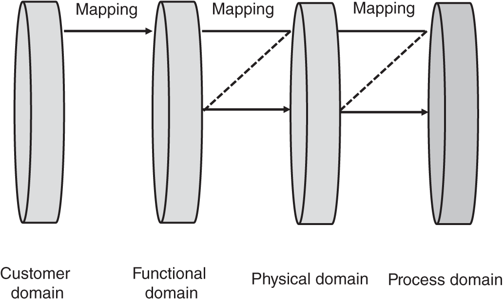
Figure 7.1 The fundamental concept of axiomatic design.
In a large‐scale problem, matrix‐based methods are difficult and time‐consuming to handle, but function/means tree is more suitable. This method is also used for functional decomposition, allocation to means i.e. components to fulfil the requirement and concept generation. The function/means tree has hierarchical structure functions and means on various levels. It can also be used to represent alternative solutions, from which a final candidate can be determined (Johansson and Krus 2006). Since integrated modular avionics architecture has many software applications, and hardware as well as dependencies among them, this allocation‐based design technique is more appropriate. Figure 7.2 depicts a generalised inheritance mechanism which is called generic object inheritance enabling a quick reuse and modification of conceptual product and/or solution models at any level in their hierarchical break down structures (Johansson et al. 2008).
The developed methodology, explained in Section 7.3, used this technique for avionics functional breakdown and allocation of avionics line replaceable units (LRUs) for each function. Each function, in some cases, a combination of two or three functions is allocated to LRUs (means/solutions) from different vendors. This has created a set of data which is used for investigating various architectures as well as trade‐off studies. The best allocation is based on physical and operational requirements needed. In other words, the avionics functions are assigned to components (LRUs) and components are assigned to installation locations.
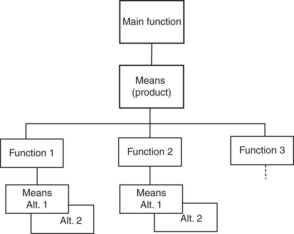
Figure 7.2 Function/means tree.
7.2.3 Integrated Development Environment
The advancement in domain specific modelling has created powerful tools for their main purposes. Many tools, however, have a limited scope of modelling and/or analysis which necessitates the need to integrate information/models from various modelling domains. To analyse and simulate a system in a large scope i.e. aircraft level, models and tools from various modelling techniques need to be integrated. For instance, an integrated system model could be models from hardware, models of embedded software, and models of the environment of the system e.g. other subsystems. In aircraft systems development, particularly avionics systems development, a set of engineering tools that are designed to work together are known as ‘integrated’. These tools will decrease the non‐productive time which is spent on user interaction with separate tools as well as transferring data among various engineering tools. Some of the most mature tools that are being used in aircraft systems development are DOORS, Focal Point, Modelica, Dymola, SCADE, MATLAB Simulink, Unified Modelling Language (UML), and Systems Modelling Language (SysML).
7.2.4 Model Management
For a complex systems design, when moving from document‐based method to a model‐based one, it is crucial to understand how to manage the set of models that have to be explained and planned. In other words, model management is to ensure that model‐based methods and tools fit into the existing development environment for aircraft and/or avionics systems. Moreover, the modelling techniques and models as well as the supporting tools need to be managed during the whole of system's life cycle i.e. every change in a model has to be validated.
7.2.5 State‐of‐the‐Art Avionics Architecture Modelling
A couple of modelling approaches are being used for avionics architectures including static modelling, safety modelling, and dynamic timing analysis. Here the emphasis is on models used in the context of IMA and DIMA architectures, and their pros and cons are addressed. Some general systems modelling approaches like UML and SysML can also be used to model some aspects of IMA architectures; however, UML profiles and their lack of discipline makes it difficult to verify, evaluate, and optimise IMA architecture automatically.
7.2.6 Key Aspects to be Modelled
The main goal in avionics system architecture modelling is to enhance the planning and the design process as well as improving the operational capability of the desired architecture. Thus, it is critical to fully understand all aspects of the avionics system architectures including the driving requirements, IMA architecture components and the process of function allocations to hardware, and hardware mapping of the components into aircraft structure. Figure 7.3 represents an overview of the IMA/DIMA architecture elements from software mapping to hardware mapping and their associated constraints and qualitative/quantitative measures.
The system layer is used to describe the functional breakdown and/or decomposition i.e. each subsystem has its dedicated technical specifications like resources (computation and storage), connectivity and capacity as well as other properties associated to IMA/DIMA architectures such as design assurance level (DAL). The aim of this layer is to identify the system tasks, logic, and connections as well as required sensors/actuators and interfaces for functional subsystems. For instance, a high lift system task/function is the extension and retraction of flaps and slats triggered by a flap lever in the cockpit. This may include a sensor acquisition, a monitoring, and actuator modules. These modules are enabled by a set of hardware components in hardware layer including common processing modules (CPMs), remote data concentrators (RDCs), and sensors.
The hardware layer is concerned with hardware devices and their configurations as well as network topology that support the functions in the system layer. The typical devices in IMA/DIMA architecture are CPMs, RDCs, input/output (I/O) modules, sensors, actuators, switches, and cables.
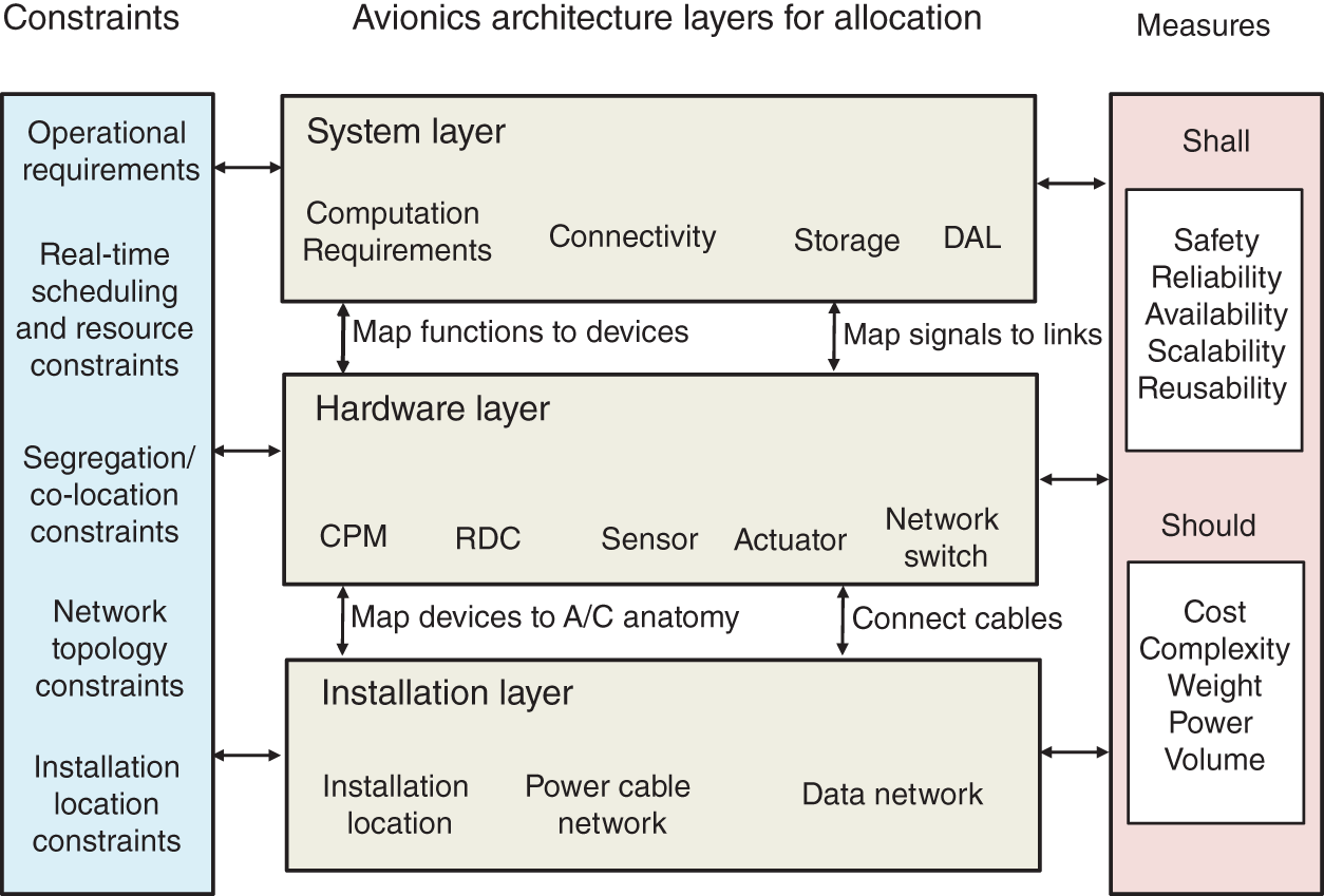
Figure 7.3 IMA/DIMA system architecture elements and design layers.
The installation layer allocates hardware to aircraft anatomy. It is indicated by installation locations and power network. The devices can be placed at different installation locations like avionics bay, cockpit, and centre and tail of the aircraft. These locations have their own constraints including mass, volume, cooling capability, number of slots, and power supply. These criteria must be taken into account for the optimisation of architecture while placing the devices in their installation locations. It can affect both the cable length and safety requirements.
All the three layers must be carefully modelled and designed by taking into account the required measuring criteria to achieve an optimised avionics architecture. In what follows some modelling techniques and/or tools are reviewed.
7.2.7 Architecture Analysis and Design Language (AADL)
Architecture analysis and design language (AADL) is one of the most popular tools in the avionics domain. It is a modelling language to describe software and hardware of critical and embedded systems. The hardware in the AADL is modelled as a composition of processors, memory, buses, and devices. Software is comprised of processes, threads, subprograms, and data. The system is comprised of an arbitrary set of software and hardware components. Several systems can be implemented. Further, components can be linked together by either signal relations or by child relations (hierarchical dependencies), for instance, assigning a process to a processor. AADL is standardized by Society of Automotive Engineers (SAE), including an extensible markup language (XML) data format and graphical representation (Feiler et al. 2006).
7.2.8 AADL‐Based Modelling of IMA
The different layers shown in Figure 7.3 have been modelled by AADL. Fraboul and Martin proposed an IMA domain model consisting of four layers including application, architecture, mapping, and execution (Fraboul and Martin 1999). The application model includes Air Radio Inc. (ARINC) 653 partitions and ports as well as their connections. The architecture layer comprises CPM and buses. The application layer is bound to the architecture in the mapping layer. Finally, it is viable to automatically derive discrete even simulations by combining layers with the execution layer, which holds run‐time information on hardware and software.
Delange et al. also proposed an AADL scheme to model ARINC 653 partitioned systems (Delange et al. 2002). The scheme defines how ARINC 653 partitions, processes, communication ports, health monitoring as well as ARINC 653 hardware is modelled. It defines the AADL classes to use and set of attributes. The proposed rigid modelling provides a derivation of executable dynamic schedule models. The approach is used for model‐based verification of system and ARINC 653 OS layers. Further, a simulation approach of configured IMA system down to hardware is given by Lafaye et al. (2011). This paper shows how to transform AADL models in SystemC models. SystemC models are executable and used for hardware software interaction simulations. A unique one‐to‐one mapping between AADL classes to SystemC modules is given. Moreover, with the rigid modelling rules, transaction level SystemC models (TLM) can automatically be derived. Also, a demonstration shows how to verify processor and memory load limits on an IMA device loaded with system software over time.
7.2.9 Mathematical‐Based Modelling of IMA
Förster et al. proposed π‐calculus as a textual modelling language for avionics and IMA systems specification and verification (Förster et al. 2003). π‐calculus is a formal mathematically motivated process specification language. The modelling elements are processes and their communication. The execution of π‐calculus allows formal verification of the logical correctness of the modelled systems. The proposed model covers functional and communication specifications as well as hardware and network topology. The automatic derivation of specification is enabled by specifying software–hardware bindings. The simulation of this implementation is used to verify complex software/hardware systems.
In addition to IMA devices, avionics networking i.e. Aircraft Data Communication Network (ADCN) modelling has also been modelled in some literatures. Avionics full duplex switched Ethernet (AFDX) end‐to‐end delays are analysed by Charara et al. where a comparison is made of network calculus, the queuing network modelling approach, and model checking (Charara et al. 2006). Network calculus is a mathematical model expressing each network node by queuing capability and queue size. For given message sizes and arrival rates, this can be propagated through the network automatically. The queuing approach builds up networks from basic building blocks like links, buffers, and multiplexers. Underlying behaviour and configurable properties of each block allow a simulation of network traffic to obtain delay information. Model checking uses timed automata to express network nodes. Comparing the three approaches, the precision goes up from network calculus to model checking as the calculation effort does.
Lauer and Ermont also proposed a modelling and simulation approach to verify latency and freshness requirements in AFDX networks based on the tagged signals model (Lauer and Ermont 2011). The loaded IMA systems are modelled as processes and signals transmitted over timed channels. IMA devices with applications are expressed as processes. AFDX links are timed channels. The transforming tagged signal models are expressed in mathematical optimisation problems in which end‐to‐end latency and freshness parameters can be calculated for different network setups. The proposed approach is applied on a flight management system (FMS) composed of a switched AFDX network, RDCs, and the cockpit panels.
7.2.10 General Assignment and Mapping Problem
The assignment problem answers the question of how to assign m (jobs, students) items to n other items (machines, tasks). Since there are many possible ways to perform this assignment, it is then defined as an optimisation problem to achieve the best suited assignment for the problem (Burkard et al. 2009). The mathematical model is defined as follows:
Let xij = 1 if task i is assigned to person j and 0 otherwise. Let Cij be the cost of assigning i to j. Then, the objective function is to minimise the total cost of the allocation which is to
Each task goes exactly to one person and each person gets only one job. These are given by the following constraints:
The decision variable is defined as a binary integer programming (BIP), i.e. xij ∈ {0, 1}.
One of the applications of assignment and/or mapping problem is the allocation of software applications to processors in distributed computing modules (Bokhari 1987). The objective in these problems is that a set of tasks is assigned to processors for the shortest time execution. The assignment can be either static or dynamic. The processes are restricted by resources like calculation time, memory, or bandwidth. The network can also be considered. In other words, the communication topology plays a significant role when optimising the overall execution time. The assignment problem classes differ in multiplicity of assignment, the number and type of resources, and the number of assignment layers, constraints, and the objective functions. This problem is well‐known to be NP‐hard in most cases, i.e. it cannot be solved by a deterministic algorithm in certain amount of time.
In other words, the optimal solutions can be found by an exhaustive search, yet there are nm ways to assign m tasks to n processors, for instance, the search is often impossible. Therefore, optimal solution algorithms only exist for small problems. This combinatorial optimisation problem can be solved by exact and heuristics methods which results in optimal and suboptimal solutions respectively. The best solution algorithm depends upon the problem properties and the problem size. The exact methods usually work for small instances, yet for large instances, heuristics are created. Two examples of distributing computing systems defined as static assignment problem and solved by heuristics are given below.
Lo created a three step heuristics method for assigning tasks to processors to optimise overall execution time and communication cost. First, tasks are assigned in an artificial two processor network, which is optimal but not complete. Thus, it is repeated iteratively with updated processor and network capacities. Finally, the unassigned tasks are assigned by trial to the first capable processor. They managed to get great objective values in short runtimes for a group of 34 tasks and six processors (Lo 1988). Kafil and Ahmad used the A* algorithm to solve the same problem. The algorithm is a non‐deterministic global search algorithm using a search tree to calculate the costs of visited parts. The method further was extended by reducing the number of nodes, which happened by an initial guess. The results for 20 tasks and four nodes have been calculated in very short runtimes (Kafil and Ahmad 1997).
The distributed systems assignment problems are basically similar to the issues in IMA and DIMA architectures design. For example, assigning the avionics functions to IMA devices is an assignment problem. Also, software mapping is a static assignment problem. Moreover, IMA task assignment depends strongly on resources like power, memory, and I/O types. The safety requirements are also very important. Similar examples of these types of problem can be found in operations research. In what follows the IMA related works are overviewed.
7.2.11 An Overview of IMA Architecture Optimisation
The aim in avionics architecture optimisation is to support the IMA design process with automated and/or semi‐automated architecture generation. To achieve this goal, the IMA design problem must be expressed formally and mathematically. A mathematical algorithm is then applied to the model to perform an exhaustive design space exploration. The input and output of the model is IMA architecture models. This enables designers and/or decision makers to investigate various possible architectures as well as the optimal one.
The automated design and sizing of IMA architecture is a relatively young field of research. However, the idea of how to make the best use of resources, resource allocation problem, in computer science and general assignment problems in operations research are very old. In addition, automated design and optimisation are also carried out in other industries and disciplines like space, automotive, economics, and infrastructure planning. In what follows an overview of literature on general distributed computing system optimisation as well as IMA architecture optimisation is given.
Over the past decade, the implementation of IMA architecture has been widely used by aircraft manufacturers. IMA architecture optimisation emerged with the creation of the first IMA systems. In early years, the priority was on validation rather than optimality. The main issues in IMA architectures are on processor scheduling and finding safe and reliable mappings of functions and signals in networks. Many approaches previously have been studied for model‐based design and verification of IMA architectures. Most of them are related to one hardware device or a single avionics system. Only a few approaches exist that handle the whole software and hardware architectures, multi‐devices and multi‐applications, as well as spatial distribution.
Salomon and Reichel developed a static model for the automatic design of IMA architecture i.e. the allocation of avionics functions to IMA devices and placing the devices in aircraft structure (Salomon and Reichel 2013). The model provides some automation in IMA design process by applying an optimisation algorithm and focuses on safety evaluation. The model expresses logical, physical, and structural aspects of avionics systems. It includes propagation failure layers, function instantiation, hardware, hardware types, and geometry. The failure propagation model expresses system logic in terms of functions and connections. The failure propagation is dealt within the three stages including ‘ok’, ‘passive’, and ‘out of control’. Signals and components are ‘passive’ if an error is detectable and ‘out of control’ if not.
The hardware types define all the components with their technical specifications like failure probability and cost. These components are then allocated to a geometry model. The function instantiation expresses the operational system which comprises multiple instances of the functions and connections from the failure propagation model. The redundancy level is also defined in a function instance model which represents the functions of the failure propagation model. The complete model provides the automatic derivation of fault trees and the computation of reliabilities with some simplification like excluding failures canceling each other (Salomon and Reichel 2011). The optimisation method used is a conventional genetic algorithm (GA), and is applied to flight control system architecture. The method and the algorithm do work well for small and medium architecture like flap control system; however, for large‐scale architecture e.g. the whole flight control system with a high redundancy level, it does need an improvement to produce optimal results.
Dougherty et al. in Vanderbilt University in collaboration with Lockheed Martin developed a tool called ScatterD to optimise embedded flight avionics systems (Dougherty et al. 2011). The domain studied is mission computer and flight control systems. The deployment problem is expressed as a multi‐resources bin‐packing problem. In other words, the computer aided design tool deploys software applications to hardware while satisfying a number of complex constraints including processing time and real‐time scheduling like processor time, memory size, and bandwidth. The optimisation algorithm implemented is a hybrid heuristics, genetic algorithm (GA), and particle swarm optimisation (PSO). The tool manages to reduce the required processors and network bandwidth consumption. The installation location of hardware and the operational capability of the system architecture are not studied.
In another literature, Manolios et al. from Georgia Institute of Technology in collaboration with Boeing for B787 project developed a general framework called component‐based system assembly (CoBaSA) that implements a constrained component assembly technique (Manolios et al. 2007). The main objective of the tool is to create an environment for construction of large industrial systems by integrating components, particularly COTS components. CoBaSA software includes an expressive language for component interfaces, properties, and system‐level and component‐level constraints. Further, it uses a pseudo‐Boolean solver to solve the constraints using SAT‐based method. The tool enables automatic solving of system assembly problem directly from a system requirement. The tool mainly contributes to a greater reliability, lower cost development, shorter development cycles as well as less testing and validation in system design and integration.
CoBaSA is further used for the integration of IMA avionics architecture components for the Boeing 787 Dreamliner. The assembly problem of IMA architecture involves mapping of avionics function to line replaceable modules (LRM), mapping of LRM to cabinets, mapping of RDCs to switches as well as sensors and actuators. Moreover, system architects have to consider some constraints including worst case execution time (WCET), I/O timing, memory, latency, network jitter, and so on. The implementation of CoBaSA has hugely reduced the assembly time for Boeing compared to their current methods.
Shi and Zhang also developed a tool for avionics integration optimisation using mathematical programming (Shi and Zhang 2016). The tool is created in three steps called system organization, system integration, and requirement analysis. First, the system organization is based on linear programming (LP) and is used to select the best vendor products according to the system performance requirements like minimising and/or maximising a particular cost function. In this step, suitable devices are selected for the architecture. The properties considered for the devices to be selected are performance, weight, size, power, processor unit, and DAL. Then, in the system integration phase, designers are able to form the optimal architecture with all the constraints defined by applying optimisation algorithms.
The algorithm used in this work is GA and PSO where users can select the algorithm for their problems. The requirement analysis further verifies the integration design by Boolean logic. The major requirement assessed in the paper is safety. Since the safety requirements are defined as Boolean, a satisfiability modulo theory (SMT) solver is used for requirement verification. The tool is basically developed in Java, and is eclipse‐based. In all steps, the user needs to manually choose the safety objectives and evaluation algorithm. Spatial distribution of avionics modules in aircraft structure is not studied in this work, and the human machine system is not taken into account in the model for safety assessment.
Zhang and Xiao modelled the DIMA as a cyber physical system (CPS) integration scheme with physical layer and function layer. The physical layer focuses on mapping of CPM and RDC into predefined locations including avionics bay, cockpit, centre, and tail (Zhang and Xiao 2013). The function layer is about the allocation of tasks/functions to CPM, RDC as well as sensors and actuators. The integration constraints defined are influenced by the maximum resources available in each location including mass, slot, and cooling capability for physical layer. For the functional layer, constrains are related to calculation resources like memory and segregation constraints of functions.
To implement the scheme and apply multi‐objective optimisation for the DIMA system, software based on MATLAB was developed. The multi‐objective optimisation problem is solved by using an improved lexicographic optimisation technique for minimising the weight and maximising the reliability. The model represents that the reliability measure in optimisation is improved. Moreover, the comparison between IMA and DIMA shows that DIMA proves a better performance in reliability.
Salzwedel and Fischer presented a new methodology for optimising avionics architecture at aircraft level (Salzwedel and Fischer 2008). The proposed method is developed to deal with bounded and statistical uncertainties of early design stages related to the components of an architecture. To handle these complex tasks, two techniques have been employed. One technique is used to develop an automated design at system level that tackle the uncertainties, and the other one is developed for system level optimisation of avionics architecture and function. The automated design provides an environment for simulation by connecting to a database of architecture components and their connection information. The Monte Carlo method is also used to handle components uncertainties. The process comprises modelling of the architectural components and network system, automated mapping of avionics function into architecture, developing an XML database format, and architectural optimisation at aircraft level. The approach managed to minimise cost, weight, and cable length, and maximise availability and generates an XML description of the optimised IMA architecture. The optimisation results in reducing wiring by 68%, cost by over 78%, and increasing availability by several orders of magnitude.
Annighöfer et al. developed a model‐based methodology for architectural design of a DIMA architecture. A meta‐model is defined for DIMA architecture design from system requirements and aircraft anatomy up to functional allocation to IMA hardware devices, networking, and physical installation locations. As aircraft systems require calculation power to execute their logic, and I/O interfaces to connect their peripherals (sensors and actuators), they must meet safety and performance constraints like reliability and signal latencies which are also modelled. A number of cost functions are also defined to evaluate the system architecture. These are mass, ship set cost (SSC), operational interruption cost (OIC), initial provision cost (IPC). This work is of one a few works that is suitable for aircraft modelling. In Annighöfer et al. (2011) the IMA platform which is the combination of hardware, the system applications, signals, and peripherals are modelled in different layers including software mapping and hardware mapping. The software mapping is the allocation of avionics functions to IMA hardware, and the hardware mapping is the allocation of hardware to installation locations in aircraft structure. The system constraints defined are peripheral, segregation, atomic, latency, devices, installation locations, and power constraints.
Moreover, they proposed a novel method for automated device type selection, sizing and mapping of IMA architecture based on binary programming (BP) (Annighöfer et al. 2013). The tool is developed in eclipse modelling framework (EMF). The optimisation is implemented in MATLAB. The model employs a combinational multi‐objective solver including Pareto front, branch‐and‐cut algorithm, and a genetic algorithm (NSGA‐II). Pareto front shows a better performance in optimality. For single objective, solving a COTS solver like CPLEX and GUROBI is used as well. As a case study, the method is applied to four aircraft systems including bleed air system (BAS), pneumatic system (PS), ventilation control system (VCS), and over heat detection system (OHDS). The optimisation problem is solved for mass and OIC as objective functions. The results show a great improvement in mass and OIC compared to manual design.
They managed to extend their model further to signal routing and network topology. An AFDX topology is described by devices and links, and presented as an undirected graph (Annighöfer et al. 2014). To achieve the optimal topology, the problem is formulated as binary programming (BP) which is a combinatorial optimisation problem. The network topology evaluated by costs like mass contribution while satisfying a number of constraints. The topology mass is calculated from the mass of all switches used and the cable mass of all links. The optimisation problem is solved for mass and OIC as objective functions. The results show an improvement in signal routing and network topology. The method is used to optimise full or sub‐parts of avionics architectures for certain objectives such as mass and cost while considering system requirement.
Lee et al. developed a scheduling tool and algorithm for optimisation of airplane information management system (AIMS) Boeing 777 cabinets (Lee et al. 2000). AIMS is a time synchronised distributed computing system which includes several processors and I/O boards. The proposed algorithm calculates the time scheduling for all partitions, tasks, and bus messages. The objective is that all partition and task deadlines are held and the capacity of processors and buses is not exceeded. They came up with a two‐level algorithm creating the processor's schedules first and then calculating the bus schedule.
Zhang used mixed integer linear programming (MILP) to find virtual link (VL) trees in an AFDX network (Zhang 2008). This work illustrates how to formulate linear constraints and binary variables such that a consistent routing tree from each source node to each destination node is retrieved. The objective is an overall low bandwidth utilisation of AFDX links. It is implemented for a topology of eight nodes that up to 1600 VLs can be routed in four hours. However, global optima are not retrieved.
Bauer et al. in Airbus Toulouse developed a decision‐analysis tool for the optimisation of fly‐by‐wire flight control system architecture of airliners (Bauer et al. 2007). The tool for fly‐by‐wire flight control system architecture postulates a combination of actuators, power circuits, and flight computers for each control surface. Different actuator technologies are considered including servo‐control (S/C), electro hydrostatic actuator (EHA), and electrical‐backup hydraulic actuator (EBHA). The objective is to select the system architecture that keeps the weight as low as possible while fulfilling safety and technological constraints. They chose branch‐and‐bound algorithm to solve this discrete optimisation problem for Airbus A340 roll control system architecture. Two scenarios are solved including 3H in which three hydraulic circuits power the flight control actuators and 2H‐2E where two hydraulic and two electrical circuits power the flight control actuators. The resulting architecture weighs 3.1 kg less than the reference architecture.
Literatures reviewed above were the most relevant published works related to automated IMA architecture design and optimisation. The scope of each approach, however, is limited to a certain aspect. The baseline for all of them include problem formulation, constraint definitions, and solving techniques like integer programming (IP), BIP, and mixed integer programming (MIP). Nevertheless, examples can be found in other industries as well.
7.2.12 Architecture Design and Optimisation in Other Industries
Similar topics from other industries like space and satellite systems are also popular. Since determining the optimal placement of avionics boxes on the spacecraft is a difficult task which is normally performed manually, Jackson and Norgard developed a tool to optimise avionics box placement (Jackson and Norgard 2002). This has been defined as a multi‐objective optimisation problem for optimising the placement of avionics boxes on the exterior panels of a spacecraft in which multiple cost functions and constraints must be satisfied. The objectives are to minimise the amount of harness wiring and the length of radio frequency (RF) cable runs while keeping the thermal loading and mass distribution across panel within acceptable limits. The input information into the problem are avionics boxes dimension, masses, power dissipation, mounting location of fixed components, connectivity between boxes and interconnection priority weighting. Further, a simulated annealing (SA) algorithm is proposed to solve the problem. SA reaches the optimal solution by perturbing the current best solution to explore more of the solution space.
Fabiano and his colleagues also developed a tool for the spacecraft equipment layout since the decision‐making of where to place electrical equipment is a difficult task while taking into account many factors like position of centre of mass, moment of inertia, heat dissipation, and electro‐magnetic interference (EMI) and integration issues at the same time. This task is usually done by a group of system engineers which takes time and as soon as a feasible solution is found, it becomes the baseline. In other words, all possibilities and layouts are not explored completely and the solution is not necessarily the optimal one. In this paper, a tool based on Excel is developed that employed optimisation techniques which provides the system engineering team and easier way to explore the layout conceptual design space. The algorithm used is M‐GEO which is a multi‐objective algorithm. Finally, decision‐making criteria are used to select solutions from the Pareto frontier. Works with similar concepts can be found in literatures (Yang et al. 2016; Dayama et al. 2020; Sousa et al. 2013).
Annighöfer also developed a formal mathematical‐based model for the European space launcher ARIANE 5 to upgrade its avionics systems as well as future launchers (Annighöfer et al. 2015a; Annighöfer et al. 2015b). Since the ARIANE 5 launcher was first developed in early 1990s, it has a federated avionics architecture, and its avionics systems may not be necessarily optimal with respect to the current technological advancement and requirements. The proposed architecture has used the IMA architecture concept. Moreover, the avionics architecture design is formulised as a binary programming which includes function allocation to IMA devices and mapping the device into an installation location while satisfying a number of constraints like power, mass, and segregation. Twenty installation locations are available for IMA devices and 158 locations for peripherals (sensors and actuators). MIP and COTS solvers like CPLEX and GUROBI are used to solve the optimisation problem. The results led to a huge optimisation in mass, power consumption, and reduction of cable length.
A similar concept from automotive industry is a commercial tool called PREEVision. It is a model‐based design of electrical and electronic (E/E) architectures for the automotive domain (PREEvision 2020). The main goal of the tool is to provide a component database which supports automatic design. The model consists of functional, component, and installation layers as well as the evaluation of requirements. The components are automobiles' electronic control unit (ECU) and data buses like controller area network (CAN). The functions are then assigned to an ECU, and the ECU is assigned to installation locations. Moreover, the function signals that are assigned to wires or buses can be automatically routed. The complete model and tool enable different instantiations of the same architecture.
Hardung in his PhD dissertation developed a framework for the optimisation of the allocation of functions in automotive networks (Hardung 2006). Multiple objectives were defined including costs and busload for optimisation, while a number of constraints like memory consumption, I/O‐pins consumption, timer consumption, and bandwidth availability are met within acceptable limits. In other words, the hardware is assumed fixed, and the software components are to be allocated to ECUs. A database model in structured query language (SQL) is built to store all relevant information including ECUs' technical specifications like the weight of ECU and wiring harness, cables, cost, and their functional links. The model is then implemented for central door locking and keyless entry where the details of the architecture is shown which include network topology, resources, costs, weight, busload as well as supplier complexity. The supplier complexity is defined by the minimum number of suppliers involved in the development of the ECU. This is transferred into a set‐covering problem. The optimisation algorithm proposed is ant colony optimisation (ACO) which is also compared to evolutionary algorithm (EA) and is shown that ACO is faster than EA at the beginning. However, after a while, ACO cannot find better solutions. While EA is slow at the beginning, it is continuously improving in later phases. Due to better performance, at the end the ACO is selected as the final approach.
7.2.13 Comparison of Modelling Approaches
All the above approaches can be utilised to express IMA architecture in a certain scope. All of them are driven by mathematical programming which can formulate the IMA design problem and speed up the development process automatically and/or semi‐automatically through simulation or formal verification. What is common among models is their formulation i.e. the overall definition of the problem mathematically. This includes decision variables, objective functions, and constraints. The decision variables are defined in various forms like IP, binary programming (BP), and MIP. Also, the objective functions defined are different, for instance in Salomon and Reichel (2011) and Zhang and Xiao (2013), the objectives are related to improving reliability and safety of the architecture whereas in Dougherty et al. (2011), the objective is to minimise the hardware (processor) and the required network bandwidth. The main objective functions in Annighöfer et al. (2014) and Annighöfer et al. (2013) are to minimise weight and costs.
Moreover, models in Salomon and Reichel (2013), Manolios et al. (2007), Annighöfer et al. (2011), and Salzwedel and Fischer (2008) are capable of expressing aircraft‐level architecture which is within the scope of this research as well. The other issues are related to the separation of software and hardware as well as the level of automation. Software mapping and/or hardware mapping alone cannot express the complete model of an architecture. Automatic design is only addressed in Annighöfer et al. (2013) and Salomon and Reichel (2013). Salomon and Reichel (2013) mainly focuses on finding redundancy structures and lacks resources for installation location. Further, the types and the number of constraints in different models vary. A thorough modelling of IMA architecture which proposes various cost functions and constraints can be found in a patent by Airbus (Minot 2010) in which constraints are formalised by a set of linear inequalities. However, the most common constraints studied in literatures can be classified as peripheral, segregation, latency, power, and installation location constraints.
In conclusion, linear programming which is a widely used technique to express real‐world problems into mathematical forms as used in literatures is selected in this research as well. The problem of IMA architecture optimisation is defined as an assignment problem in that it is to assign the best avionics LRUs/LRMs from database to the proposed integrated architectures. A set of costs functions are defined and constraints are expressed in inequalities forms. The decision variables are defined as binary variables. The contribution of this research into modelling is adding the volume and weight constraints to the architecture as well as introducing the operational capability as a new cost function.
7.2.14 Comparison of Optimisation Methods
Linear programming (LP) problems, in general, can be solved by many algorithms. However, in IMA avionics architecture as well as many other aircraft systems architectures, the variables are usually defined as either IP and/or binary programming (BP). IP problems are not easy to solve and are known as NP‐hard discrete combinatorial optimisation problems. In other words, they cannot be solved in polynomial time due to the vastness of the solution space (Galli 2018; Jensen 2002). IP problems can be solved by three different algorithms:
- The exact algorithms guarantee optimal solutions, but they may need a huge number of iterations. They are branch‐and‐cut, branch‐and‐bound, dynamic programming algorithms, Boolean satisfiability, and decomposition.
- The heuristic algorithms guarantee sub‐optimal solutions, but the quality is not guaranteed. While the running time may be polynomial in some cases, they may find a good solution fast. They are like greedy algorithms, local search, meta‐heuristics (PSO), Tabu search, and simulated annealing.
- The approximation algorithms provide suboptimal solutions in polynomial time and the sub‐optimality has a bound. They are like linear programming retaliation and Lagrangian relaxation.
The exact methods are usually suitable for small‐scale problems, yet for large‐scale problems heuristics are developed. The assignment problem, in particular, which has been used to define software/hardware allocation, installation location, and task assignment is a branch of LP and IP problems. One particular example of using IP in aircraft avionics fleet upgrade optimisation can be found in Guerra et al. (2016). Most of the other task assignment problems in IMA architecture (e.g. Lo 1988; Kafil and Ahmad 1997; Salomon and Reichel 2013; Dougherty et al. 2011) are combined with time constraints for scheduling and network transmission. They all used heuristic methods like evolutionary algorithms (EV) including GA, NSGA‐II, PSO, and ACO for these discrete optimisation problems. There is no literature that has compared these methods in IMA architecture optimisation; however, the performance of ACO and PSO are reported to be faster than the GA (Hardung 2006).
The other categories use COTS solvers like SAT‐solver, CPLEX, GUROBI, and GAMS. In Sagaspe and Bieber (2007), Carta et al. (2012), Manolios et al. (2007), and Annighöfer et al. (2014), COTS solver is used and results are compared to heuristic methods. In many cases, the COTS solver results are more accurate than heuristics.
In conclusion, the problem, in this study, is defined as an assignment problem which is a combinatorial optimisation problem i.e. very large feasible solutions exist. To solve this problem, the branch and bound algorithm which is a widely used algorithm for solving large scale NP‐hard combinatorial optimisation problems is selected. Moreover, the PSO algorithm is also implemented to compare the results using a weighted sum method (WSM) as well as solving the multi‐objective optimisation problems for finding Pareto‐frontier.
7.3 Avionics Integration Architecture Methodology
The established framework and method presented here is realised based on industrial processes and Cranfield University's internal projects in Aerospace Vehicle Design (AVD) group as well as avionics network and architecture lecture notes (Seabridge 2017) and other aircraft flight deck and systems documents (Airbus 1998; Airbus 1999; Airbus 2011; Airbus 2006; ATR 2015; Cessna 2000; BAE Systems 2007). Figure 7.4 represents an overview of the framework.
Based on aircraft level avionics requirements, the avionics system integration and architecting starts from a top‐level functional decomposition to provide the framework for the avionics systems design and integration. This leads to the equipment specifications with every requirement being satisfied by the equipment performance parameters and/or operational capabilities. In other words, for each avionics function, at least three avionics LRUs are investigated from various vendors. The operational capability of each LRU is evaluated separately against a set of criteria using multi criteria decision‐making (MCDM) method, simple additive weighting (SAW). Further all the technical specifications of avionics LRUs as well as their manufacturers are recorded in a database. Finally, the proposed initial system architecture for the automatic flight control system (AFCS) architecture and the whole avionics system architecture are modelled using mathematical programming. The problem is defined as an assignment problem i.e. it is to assign the best avionics LRUs from the database while satisfying a number of design constraints including mass and volume in installation locations.
The optimisation problem is then solved by applying branch and bound algorithm for single objective cost functions and PSO for multi‐objective cost functions. The cost functions defined here in this case study include minimising the overall weight of the architecture, minimising volume, minimising power consumption, maximising the reliability and operational capability as well as trade‐offs studied between these cost functions. The proposed method is not developed for a specific aircraft type, and it is meant to be a general method that can be used for any aircraft type and/or architecture. However, the proposed avionics architecture is similar to a short to medium haul civil aircraft architecture which is used here as a case study. The proposed architectures have used the concept of IMA architecture although they are not fully integrated.
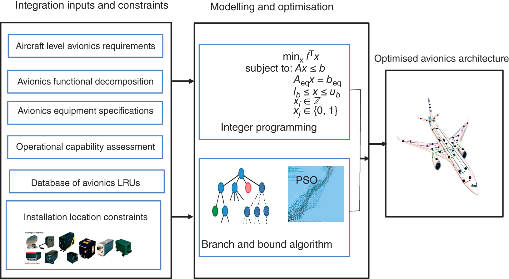
Figure 7.4 Avionics integration optimisation framework.
7.3.1 Aircraft Level Avionics Requirements
Requirements engineering is essential for creating an acceptable avionics system. The designed avionics system cannot perform as expected by the customer unless the customer requirements as well as other stakeholders' requirements and related regulations and standards are well documented and understood by designers. The major driving requirements are from safety, mission, cost, and certification perspectives. In other words, a variety of technical and functional requirements for on‐board avionics equipment have to be captured which are comprised of the following generic documents:
- Airworthiness requirements including the requirements related to aircraft equipment and systems as well as international airworthiness standards like CS‐25, FAR‐25, CAR‐525, etc.
- Functional requirements for the on‐board aircraft equipment
- Safety requirements
- Reliability requirements
- Avionics network and interface requirements
- Installation and environmental condition requirements
Here, the focus is on the communication, navigation, surveillance (CNS)/air traffic management (ATM) functions required to be on‐board the aircraft. In other words, the requirements captured are mainly from regulatory documents. The functions that the avionics systems are expected to fulfil are shown in Figure 7.5 and they are meant to meet all CNS/ATM requirements as well as FANS‐1/A. It should be noted that all the future air navigation system (FANS) and/or CNS/ATM requirements here are derived from an LRU perspective. The functional breakdown shown can be generally attributed to any civil aircraft.
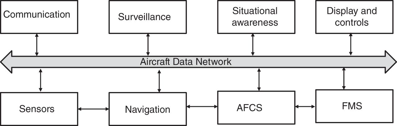
Figure 7.5 Avionics datum functional architecture.
The avionics requirements are concerned with the functional capability of avionics equipment on the aircraft. It is only after this requirement statement that the avionics design team can justifiably determine an equipment list. Then, for each item in equipment list, equipment technical specifications can be prepared. The operational capability required within each function is outlined further in detail in avionics technical specifications and operational capability assessment phase. The following requirements are obtained from the operational requirement of civil aircraft (EUROCONTROL 2017; Airbus 2007). The specific requirements are related to CNS and ATM systems as well as data transmission. The proposed architecture is to meet basic CNS/ATM requirements as well as improving operational capabilities by implementing new technologies like head‐up display (HUD) and enhanced vision system (EVS) among others.
Table 7.1 shows the capabilities that are required for the proposed avionics architectures, and further these capabilities are evaluated from an LRU perspective. In other words, some capabilities are embedded as software within a particular LRU e.g. required navigation performance (RNP) and required time of arrival (RTA) are loaded in FMS and/or multi‐function display unit (MCDU). Moreover, the accuracy and performance of some of these capabilities are further classified that determine the operational capability of avionics systems at aircraft level. The definition and classification is taken from a range of aviation international rules and regulations including International Civil Aviation Organization (ICAO) Doc 4444: PANS‐ATM, ICAO Annex 2, 10, and 14 among others (ICAO 2007; ICAO 2013; ICAO 2005). The avionics systems are classified in three main groups including communication, navigation, and surveillance.
The next column in Table 7.1 is related to avionics capabilities. These capabilities are defined from an LRU perspective. However, in some cases, some avionics capabilities are loaded into an LRU as software. Also, some LRUs are investigated that are capable of doing more than just one avionics function (e.g. traffic/terrain/transponder collision avoidance system [T3CAS]) which is an advanced integrated surveillance system featuring a traffic alert and collision avoidance system (TCAS), terrain awareness warning system (TAWS), and Mode S transponder with automatic dependent surveillance‐broadcast (ADS‐B).
7.3.2 Avionics Functional Decomposition
Functional decomposition is a technique used for describing an avionics system in very general terms. The avionics requirements are divided into a set of ‘top level’ functions. The process seems to be straight‐forward, however, there is no clear‐cut way of doing this. Figure 7.6 shows the functional breakdown adopted as the datum functional architecture from an LRU perspective. This decomposition evolves from the operational requirements of the aircraft which determines the functions needed.
Table 7.1 Aircraft level avionics systems requirements.
| Avionics systems | Avionics capabilities | Explanations |
|---|---|---|
| Communication | 8.3 kHz VHF | VHF transceiver voice channel spacing |
| SATCOM | SATCOM Airborne radio telephone communication via a satellite | |
| CPDLC | CPDLC Controller Pilot Data Link Communications (CPDLC) is a means of communication between controller and pilot, using data link for ATC communications | |
| VDL‐M2 | VDL‐M2 VHF Data Link mode 2 is a means of communication between aircraft and ground stations | |
| Navigation | GBAS CAT I/II/III | Ground Based Augmentation System CAT I is a landing system capability known as GLS whose performance is equivalent to ILS CAT I (down to 200 ft). CAT II/III are under development |
| SBAS APV CAT I/II | SBAS APV CAT I/II Satellite Based Augmentation System CAT I is a landing system capability whose performance is equivalent to LPV minima (down to 200 ft) | |
| RTA (FMS) | RTA (FMS) Required Time of Arrival enables the pilot to define a waypoint with a specific arrival time ±30 s. If the aircraft cannot meet the 30 s requirement, the flight crew will be notified | |
| RVSM | RVSM Reduced Vertical Separation Minimum for above FL290 from 2000 to 1000 ft | |
| Autopilot/Flight Director | Autopilot/Flight Director software, which is integrated with the navigation systems, is capable of providing control of the aircraft throughout each phase of flight | |
| RNAV 10 | RNAV 10, which is designated as RNP 10 in the ICAO's PBN Manual, is an RNAV specification for oceanic and remote continental navigation applications | |
| RNAV 5 (B‐RNAV) | RNAV 5 (B‐RNAV), also referred to as Basic Area Navigation (B‐RNAV), has been in use in Europe since 1998 and is mandated for aircraft using higher level airspace. It requires a minimum navigational accuracy of ±5 nm for 95% of the time and is not approved for use below MSA | |
| RNAV 2 | RNAV 2 supports navigation in en‐route continental airspace in the United States | |
| RNAV 1 (P‐RNAV) | RNAV 1 (P‐RNAV) is the RNAV specification for Precision Area Navigation (P‐RNAV). It requires a minimum navigational accuracy of ± iron for 95% of the time | |
| RNP 4 | RNP 4 is for oceanic and remote continental navigation applications | |
| RNP 2 | RNP 2 is for en‐route oceanic remote and en‐route continental navigation applications | |
| RNP 1 | RNP 1 is for arrival and initial, intermediate and missed approach as well as departure navigation applications | |
| Advanced RNP | Advanced RNP is for navigation in all phases of flight | |
| RNP APCH | RNP APCH and RNP AR (authorisation required) APCH are for navigation applications during the approach phase of flight | |
| RNP AR APCH | RNP APCH and RNP AR (authorisation required) APCH are for navigation applications during the approach phase of flight | |
| RNP 0.3 | RNP 0.3 is for the en‐route continental, the arrival, the departure and the approach (excluding final approach) phases of flight and is specific to helicopter operations | |
| Surveillance | ADS‐B | A means by which aircraft, aerodrome vehicles and other objects can automatically transmit and/or receive data such as identification, position and additional data, as appropriate, in a broadcast mode via a data link |
| Mode S Transponder | Mode S Transponder is a Secondary Surveillance Radar (SSR) process that allows selective interrogation of aircraft according to the unique 24‐bit address assigned to each aircraft. Recent developments have enhanced the value of Mode S by introducing Mode S EHS (Enhanced Surveillance) | |
| TCAS/T2CAS/T3CAS | TCAS/T2CAS/T3CAS Currently, TCAS II version 7.1 is mandated in European airspace |
Based on this functional decomposition which is derived from aircraft level avionics requirements, an equipment list, in this case LRU, is prepared. For each avionics LRU, at least three different examples are investigated from various vendors. The recorded LRUs are different in their physical specifications as well as their operational capabilities. This then leads to the problem of choosing the best LRU in order to optimise architecture in some criteria like weight and also improve the operational capability. The initial system architecture based of these equipment lists is drawn below.
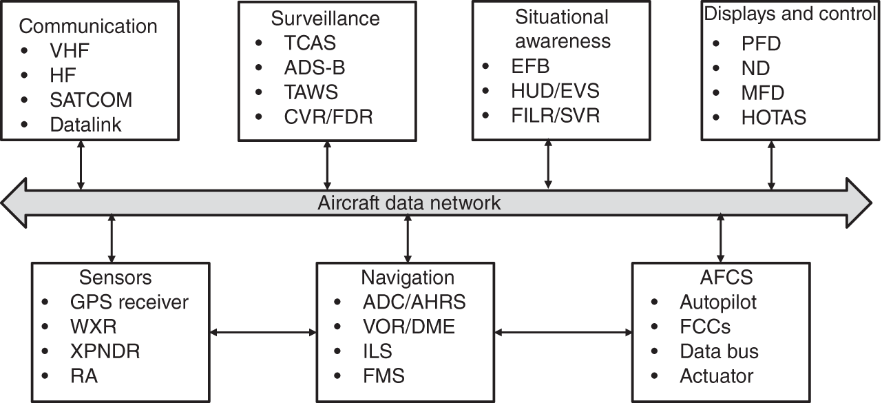
Figure 7.6 Avionics functional decomposition from an LRU perspective.
7.3.3 Automatic Flight Control System (AFCS) Architecture
Avionics system architecting is the determination of the necessary interconnections and functional interrelationships between the components of an avionics system which is a complex task. Typically, this task is shared between the airframe manufacturer and the avionics supplier to ensure that all relevant factors and implications are taken into account. The initial system architecture is adopted directly from the integrated datum functional architecture and functional decomposition. Figure 7.7 illustrates the proposed system architecture for AFCS.
The proposed AFCS guarantees three functions including autopilot (AP), flight director (FD), and yaw damper (YD). The main components are two integrated avionics cabinets (IAC) which host automatic fight control application (AFCA) and exchange data with two air data computers (ADC), two attitude and heading reference systems (AHRS), two flight control computers (FCC), and seven display units. The navigation sensors are very high frequency omnidirectional range (VOR)/instrument landing system (ILS), global positioning system (GPS) receivers, and radio altimeters (RA). This architecture in modelling is referred as the small‐scale architecture i.e. each avionics function and/or LRU will be defined as an avionics node in a network and/or architecture. Further, the AFDX/ARINC664 data bus is selected as the main data transmission system for the proposed architecture. The idea of IMA has also been implemented in two IACs. The IAC supplies resources for avionics applications including memory, I/O, and computations which are shared.
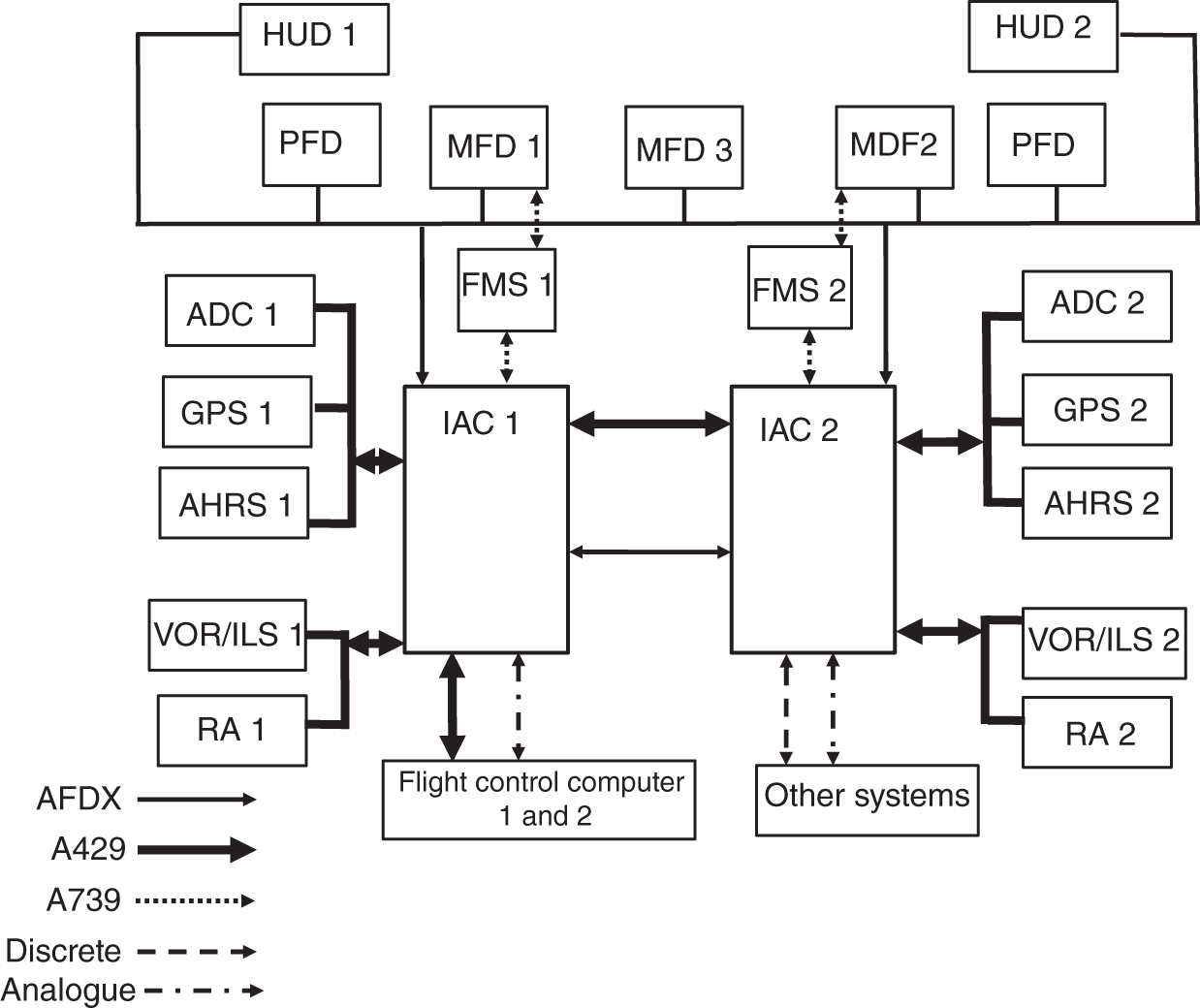
Figure 7.7 Automatic flight control system architecture.
The IACs host the following avionics applications:
- Flight warning application (FWA)
- Auto‐flight control system (AFCS)
- Centralised maintenance application (CMA)
- Data concentration application (DCA)
- Switch module application (for AFDX)
Moreover, each IAC is composed of LRMs including CPM (core processing module), different I/O types, and switch module for AFDX. CPM can host avionics applications and provide the connection to avionics data network (ADN). The various I/O types provide connections for conventional avionics that cannot be directly connected to ADN. One IAC interfaces with other aircraft systems by different means of communications like discrete, analogue, and A429. The IMA information is shown in three main systems including two primary flight displays (PFDs), three multi‐function displays (MFDs), one of which is for engine and warning display. This architecture further extended to the whole avionics system architecture as below.
7.3.4 Avionics Systems Architecture
Based on functional decomposition and the AFCS architecture, the architecture is extended to the whole avionics systems including navigation, communication, and indicating and recording systems as well as terrain and avoidance systems. Figure 7.8 illustrates the proposed avionics system architecture.
The IMA part is the same as explained in AFCS architecture. Some functional integrations are applied in that two or three functions can be performed by an LRU. For instance, TCAS, transponder mode S, and ADS‐B are integrated in one LRU called T3CAS. Furthermore, the cockpit voice recorder (CVR) and flight data recorder (FDR) are also integrated in one LRU. This means that LRUs with these capabilities are found while investigating technologies for avionics functions. This architecture in the modelling section is referred as the large‐scale architecture. The same as the small scale, the avionics functions and/or LRUs will be defined as avionics nodes in a network and/or architecture.
7.3.5 Avionics Equipment List and Technical Specifications
In order to optimise the proposed architectures and trade‐off studies, it is necessary to quantify avionics LRU physical parameters as well as their performances and operational capabilities. Based on the proposed AFCS and avionics system architectures, the avionics equipment required are as follows. For AFCS architecture, ADC, AHRS, GPS receiver, VOR/ILS receiver, RA, FCC, HUD, PFD, MFD, FMS, and two IACs. These 11 avionics LRUs are used for the small‐scale architecture optimisation.
Furthermore, for the large‐scale architecture, some other LRUs are also added including weather radar (WXR), T3CAS, electronic flight bag (EFB), cockpit and flight data recorder (CVR/FDR), satellite communications (SATCOM), and very high frequency (VHF). These 17 LRUs are considered as the large‐scale architecture optimisation problem. The technical specifications and performance description of the avionics LRUs are taken from Jane's Avionics as well as their companies' data sheet. The manufacturers are chosen according to the Flight International civil avionics directory. The physical specifications of avionics LRUs recorded are mass, power consumption, volume, and mean time between failure (MTBF). The performance and/or the operational capability of each LRU is evaluated separately to be quantified.
7.3.6 Avionics LRUs Operational Capability Assessment
The operational capability of each avionics LRU is defined as the performance parameters and capabilities that an LRU can perform. Since each avionics LRU performs different functions that provide a different capability, they need to be evaluated separately against a set of criteria related to their functions. It is very challenging to evaluate new technologies, in general, and avionics LRU, in particular as a number of criteria involved in each assessment. Generally, technology assessment steps are technology identification, selection, and evaluation. The important task in technology selection and evaluation is to establish a set of evaluation criteria. Many big companies and departments have their own method to assess technology readiness level (TRL) and selection including DOE (DOE 2015), DOD (DOD 2019), and NASA (NASA 2016). It is also common to develop a tool to do technology assessment, a good example of this can be found in literature from Georgia Institute of Technology (Kirby 2002). The main focus in these reports is how to identify the TRL; however, here the author used existing technologies (LRUs) for integration and further optimisation of avionics architecture. Therefore, TRL is not in the scope of this literature although other established processes like identification and scoping of new technologies were applied according to those very established frameworks. In particular, the selection process is the main focus as it is to select the LRUs with the maximum operational capabilities.
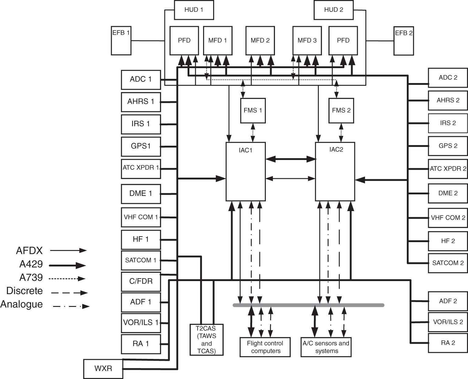
Figure 7.8 Avionics system architecture.
Since in most cases, technology evaluation and selection criteria are more than one task, a solution is to use MCDM methods to handle this complexity (Triantaphyllou 2000). The methods help decision makers in the presence of multiple and/or conflicting criteria. What is common among these techniques is a set of technology alternatives, multiple decision criteria, and the attitude of the decision makers in favour of one criterion over the other as well as the preference of the technology alternatives. MCDM techniques help decision‐makers to assess the overall performance of technology alternatives which will be further help for the optimisation of design solutions (Ching‐Lai and Kwangsun 2011).
7.3.7 Simple Additive Weighting (SAW) Method
The SAW technique is a simple and widely used method for multi‐attribute decision problems. The method is based on the weighted average i.e. weighting factors [w1, w2, …, wn] are assigned to the criteria by the decision makers. The multi‐criteria values with their weighting factors are summed into a single performance metric. SAW then selects the most preferred alternative A* which has the maximum weighted outcome as it is represented in equation below:
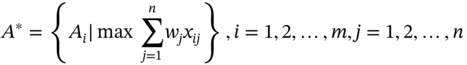
Table 7.2 Scales for technology alternative comparison.
| Intensity of importance | Definition | Explanation |
|---|---|---|
| 1 | Equal importance | Two alternatives equally contribute to the objective |
| 3 | Moderate importance | Judgement slightly favoured one alternative over another |
| 5 | Strong importance | Judgement strongly favoured one alternative over another |
| 7 | Very strong | One alternative is strongly favoured over another |
| 9 | Extreme importance | The evidence of favouring one alternative over another is of the highest possible order |
The SAW method process consists three steps:
Step 1: Building a decision matrix for technology alternatives (avionics LRUs) regarding to objectives and the relevant criteria by using a similar approach to Saaty 1–9 scale of pair‐wise comparison (Saaty 1980) presented in Table 7.2.
Step 2: Calculate the normalised decision matrix for positive criteria:
For positive criteria:
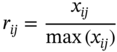
For negative criteria:
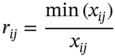
Note: In this research, all the criteria defined and considered are positive.
Step 3: Calculate the normalised weighted matrix and evaluate each alternative by the following formula:
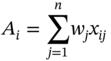
where xij is the score of the ith alternative with respect to the jth criteria, and wj is the weighted criteria.
7.3.8 Operational Capability Assessment
As mentioned before, for each avionics LRU, at least three different units from various vendors with different technical specifications are investigated. In this section, the operational capability of each LRU is evaluated by using SAW method. Since each avionics LRU performs a particular function/functions, the criteria that are defined for evaluation are almost different for each of them. Sabatini also developed a set of criteria for avionics LRUs in (2000). However, he did not use any quantitative method to evaluate these criteria. For instance, the AHRS is assessed against a set of criteria including attitude range, pitch/roll accuracy, heading accuracy, and RNP capability. For AHRS, four different LRUs are recorded that can be distinguished by their identifications (ID).
All the steps mentioned in the SAW method are applied to AHRS operational capability assessment including establishing a decision matrix, normalised matrix, and normalised weighted matrix which is led to a ranked and preferred choices. Table 7.3 shows all the criteria defined for each avionics LRU and went on the same processes to be evaluated. The selected AHRS guarantees the following performance for instance:
- Attitude accuracy: 0.1° for straight and level flight, 0.2° in dynamic situations
- Pitch/roll accuracy: 0.1°
- Heading accuracy: 0.1°
- Capability: Maintaining RNP envelop in loss of satellite.
Each assessment is done in a separate Excel sheet similar to the ARHS operational capability assessment. In this way, avionics LRUs operational capabilities are quantified as well as ranked.
7.3.9 Avionics Equipment Database
Avionics LRUs for each function/functions with their technical specifications and operational capabilities as well as the manufacturers are recorded in an Excel database. The technical specifications recorded are the ID of each LRU taken from their manufacturer identifications. The technical specifications recorded include physical characteristics of each LRU including mass, volume, and power consumption. The reliability of each LRU is also recorded by the MTBF which is used for components reliability assessment. The operational capability of each LRU which is calculated separately in operational capability assessment is also recorded.
7.3.10 Avionics Integration Optimisation Software Architecture
Based on the proposed methodology and framework for optimisation of IMA architecture a tool and/or software has been developed. Figure 7.9 represents a top‐level design of avionics integration optimisation software system (AIOSS). The tool has three main parts including a database of avionics LRUs, avionics integration architecture modelling, and optimisation algorithms. The integration constraints and inputs to the software are the avionics LRUs mass, volume, power consumption, MTBF, and the operational capability. The proposed avionics architectures have some design constraints including mass and volume in the installation locations which are also implemented in the software. Furthermore, the modelled architectures are also implemented. For the single‐objective optimisation, the software used branch‐and‐bound algorithm and for multi‐objective optimisation, PSO is used although some single‐objective cost functions are solved by both methods for comparison.
Table 7.3 Operational capability criteria assessment of avionics LRUs.
| Avionics LRU | Criteria assessment | ||||
|---|---|---|---|---|---|
| ADC | PA accuracy | IAS accuracy | Temperature accuracy | Mach number accuracy | RVSM compliant |
| VOR/ILS | Deviation accuracy | Number of channels | Capability (VOR/ILS/MB/DGPS) | ||
| RA | Height accuracy | Altitude range | Attitude range | ||
| FMS | LNAV/VNAV capability | RNP/RNAV capability | RTA capability | DataLink/CPDLC | |
| PFD | Display area | Resolution | Viewing angle | Brightness | |
| MFD | Display area | Resolution | Viewing angle | Brightness | |
| HUD | Resolution | Field of view | Approach capability | Function integration (EVS, SVS) | |
| FCC | CPU | Memory | Interfaces | Application software | |
| IAC | CPU | Memory | Interfaces | Application software | |
| WXR | Max detection range | Azimuth coverage | Elevation coverage | Capabilities | |
| T3CAS | Bearing accuracy | Range capability | Operating altitude | No. of functions integrated | |
| EFB | Resolution | Viewing angle | CPU and memory | Functions | |
| C/FDR | Recording time | Impact shock | Penetration resistance | Deep sea pressure | |
| SATCOM | Data rate | Service coverage | Functions | Capability (FANS and ACARS) | |
| VHF | Pre‐set channels | Channel change time | VDL Mode2 availability | Channel spacing (25, 50, 8.33 capability) | |
| AHRS | Attitude range | Pitch/roll accuracy | Heading accuracy | RNP capability | |
| GPS receiver | Altitude accuracy | Velocity accuracy | Position accuracy | Approach capability (SBAS/LPV or GBAS/GLS) | |
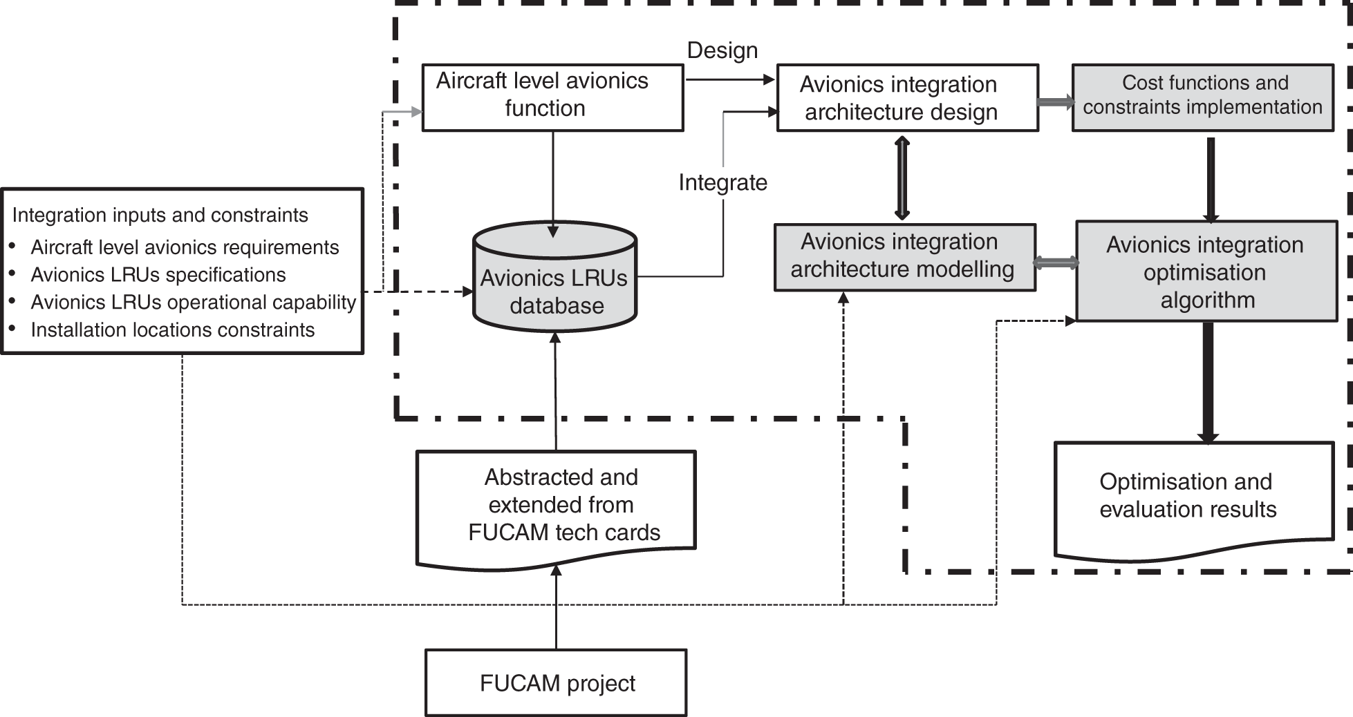
Figure 7.9 Top‐level AIOSS architecture.
Finally, the avionics integration optimisation software provides a semi‐automatic optimisation and evaluation of avionics architecture by reporting various possible architectures including minimum weight, minimum power consumption, minimum volume, maximum MTBF, and maximum operational capability. It also provides the trade‐off architectures for minimum weight and maximum operational capability as well as minimum weight and maximum MTBF.
7.4 Avionics Integration Modelling of Optimisation
The mathematical programming and optimisation algorithms have been used to model avionics architectures and provide some level of design automation in many cases. The nature of the optimisation problems in these areas of study is understood as combinatorial discrete optimisation. Due to the vastness of solution space in these types of optimisation problems, the selection of problem formulation and solving algorithms must be carefully planned in order to maintain aircraft level applications. Here, the proposed architectures are modelled and defined as an assignment problem i.e. to assign the best avionics LRUs to the architecture and installation locations while satisfying some design constraints based on some cost functions required.
All the proposed optimisation algorithms are expressed as an integer and/or binary programming. Integer and/or binary programming algorithms can be solved by COTS solvers as well as MATLAB functions. Moreover, contradicting objectives, for trade‐off studies, require multi‐objective optimisation algorithms to calculate global optimal Pareto frontier. Here, PSO is proposed for multi‐objective optimisation. The binary programming problems subject to single‐objective optimisation are solved by ‘Intlinprog’ function of MATLAB which uses branch and bound algorithm to solve the problems.
7.4.1 IMA Architecture Layers for Allocation Modelling
As earlier in Section 7.2.5 and shown in Figure 7.3, the IMA architecture has three major layers for allocation problems including function mapping to software, software mapping to hardware, and hardware mapping to installation locations. In each layer, different various constraints need to be kept. These constraints can be classified as follows:
- Resource constraints: They are related to the computing resources in software mapping to hardware and/or devices like central processing unit (CPU), memory, and power.
- Physical constraints: These are mainly related to installation locations when mapping hardware to installation locations including weight, volume, cooling capability, and the number of slots.
- Segregation/collocation constraints: These are required when two functions and/or hardware cannot be assigned to the same device and/or location due to safety or any other concerns.
- Connectivity constraints: This shows the connections between IMA devices as well as virtual links.
- Performance constraints: They describe specifications that a design must satisfy including real‐time scheduling and bandwidth.
The type of the allocation problem in this research concerns hardware mapping to installation location while keeping the installation location constraints within acceptable limits. For each function and/or functions, at least three avionics LRUs are recorded and the optimisation problem is defined to allocate the best possible LRUs to avionics architecture to optimise as well as investigate various architectures from an LRU perspective. The problem is formulated by integer linear programming (ILP) as described below.
7.4.2 Integer Programming
IP is a discrete extension of linear programming (Wolsey and Nemhauser 1999) where some or all of the variables are integer. It is also referred as ILP in which the constraints and objective functions defined are linear. A further restriction on IP is when the decision variables defined {0, 1} which is called binary programming (BP). BP in matrix notation is to optimise a linear cost function f
Subject to

where fT refers to vector transpose and x is vector of decision variables. A, b, Aeq, and beq are matrices. Integer and binary programming have the same complexity and are solved with the same algorithms like branch‐and‐bound, LP‐relaxation, cutting‐planes, branch‐and‐cut, and branch‐and‐price.
7.4.3 Avionics LRUs Assignment Problem
The proposed architectures in this chapter are modelled here. The AFCS architecture is defined as the small‐scale architecture and the avionics architecture is defined as the large‐scale architecture. In both architectures, due to the similarity of the avionics LRUs between Captain's side and the First Officer's side, only half of the LRUs are considered. In other words, they are meant to be symmetric architectures. Therefore, the binary programming variables are defined as follows:
and
The objective function defined is to minimise the weight of the proposed architecture
Further for the optimisation problem, the technical specifications and operational capabilities of each LRU are also defined as follows:
mij: The mass of each avionics LRU in node i with its associated equipment j
pij: The power consumption of each avionics LRU in node i with its associated equipment j
vij: The volume of each avionics LRU in node i with its associated equipment j
mtbfij: The reliability of each avionics LRU in node i with its associated equipment j in terms of MTBF
OCij: The operational capability of each avionics LRU in node i with its associated equipment j
Other objective functions defined by the author can be found in Radaei (2021).
7.4.4 Avionics Integration Constraints
The limited mass and volume available in installation location is very critical as explained earlier. These two constraints have been considered in modelling. In other words, for allocation of avionics LRUs to their installation locations, these two limitations must be maintained. For mass, in particular, there is also a defined target mass limitation imposed by designers in that the chosen architecture based on selected LRUs must not exceed that value. In other words, based on the defined objective functions, the selected LRUs must satisfy these constraints as well.
Mass: The mass of each avionics LRU is recorded in capturing technical specifications. Each installation location has a mass constraint which is implemented in architecture modelling for allocation of each LRU into installation locations.
Volume: The actual box dimension of each LRU is recorded in capturing technical specifications. Each installation location has volume constraint which is implemented in architecture modelling for allocation of each LRU into installation locations.
Here, three installation locations are taken into account including flight deck, avionics bay, and centre fuselage shown in Figure 7.10. Each location has mass and volume constraints and are defined as follows in avionics architecture modelling.
M: The overall maximum allowable weight of the chosen architecture
Mcockpit: The maximum allowable weight of avionics LRUs in flight deck installation location
Mbay: The maximum allowable weight of avionics LRUs in avionics bay installation location
Mm: The maximum allowable weight of avionics LRUs in centre installation location
Vcockpit: The maximum allowable volume of avionics LRUs in flight deck installation location
Vbay: The maximum allowable volume of avionics LRUs in avionics bay installation location
Vm: The maximum allowable volume of avionics LRUs in centre installation location
The assignment of avionics nodes to installation location problem has to satisfy the following constraints:
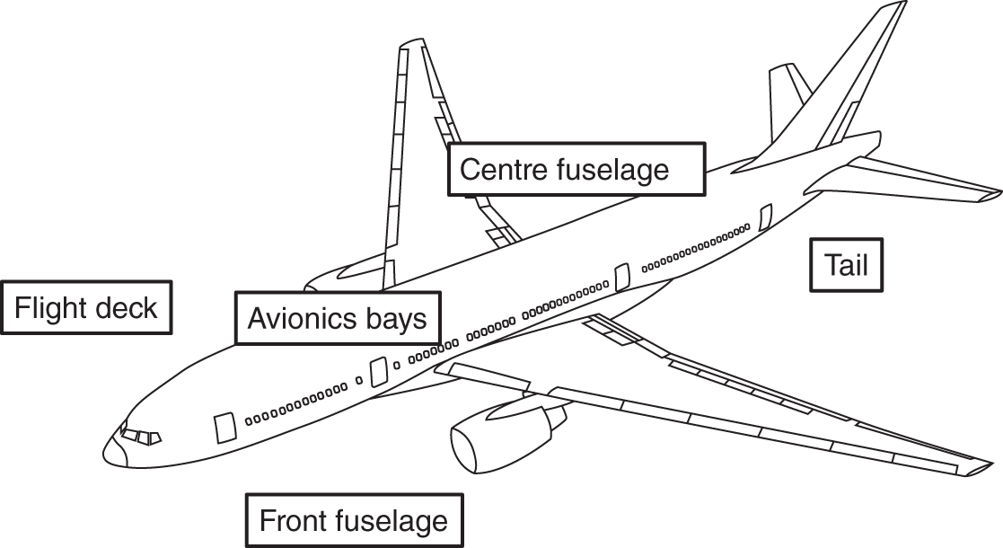
Figure 7.10 Avionics LRUs installation locations.
- Assignment constraint: each avionics node can only be assigned to one installation location i.e.
(7.13)

- Segregation and/or co‐location constraint: this constraint guarantees that two avionics LRU have to be installed separately, not in the same place. As the variables defined as binary the constraint is defined as below i.e.
(7.14)
 (7.15)
 (7.16)
 (7.17)Equation (7.14) ensures that avionics LRUs like PFD, MFD, HUD, and FMS can only be installed in the flight deck, whereas Eq. (7.15) guarantees that avionics LRUs like ADC, AHRS, GPS, RA, VOR/ILS, and IAC can only be installed in the avionics bay. Equation (7.16) ensures that ADC, AHRS, GPS, RA, and VORILS are installed next to each other and separate from the IAC. Equation (7.17) states that FCC avionics LRU can only be installed in the centre installation location.
- The mapping of avionics LRUs to installation locations has to satisfy the maximum allowable weight for each installation locations including flight deck, avionics bay, and centre i.e.
(7.18)
 (7.19)
 (7.20)
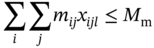
- The mapping of avionics LRUs to installation locations has to satisfy the maximum allowable volume for each installation locations including flight deck, avionics bay, and centre i.e.
(7.21)
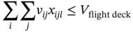 (7.22)
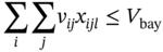 (7.23)
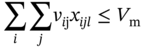
In brief, the mapping of avionics LRUs to installation locations is to minimise the weight of the chosen architecture according to the cost function defined in Eq. (7.12) while satisfying constrains equations from (7.13)–(7.23).
7.5 Simulations and Results for a Sample Architecture
For demonstration and evaluation of the proposed method, the developed avionics architectures are considered as a case study. The proposed architectures are artificial since there was no real aircraft as a reference for this study. However, the system functions, peripherals and the aircraft anatomy considered is like a single‐aisle aircraft with two engines. For the installation of avionics LRUs, three installation locations are considered including flight deck, avionics bay, and centre. Table 7.4 shows the installation locations and their related physical constraints.
Each installation location has mass and volume limits e.g. each location has a maximum allowable mass and volume to install avionics LRUs. In what follows, avionics architecture optimisation problem is solved using GAMS and MATLAB.
7.5.1 GAMS
In this section, the assignment problem of avionics LRUs i.e. the allocation of the best avionics LRUs from database to avionics architecture and mapping of avionics LRUs into their installation locations while keeping the mass and volume constraints within limits is modelled and solved using branch‐and‐bound algorithm in GAMS. Based on the cost function defined in Eq. (7.12), the objective is to select and map the LRUs into their installation locations in order to keep the weight of the selected architecture minimum. Figure 7.11 represents the results in GAMS environment.
Table 7.4 Installation location constraints.
| Installation locations | Mass (kg) | Volume (in. m3) |
|---|---|---|
| Flight Deck | 50 | 3100 |
| Avionics bay | 40 | 2500 |
| Centre | 30 | 1000 |
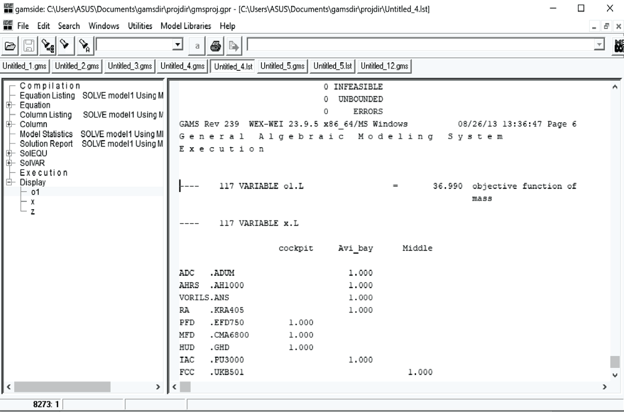
Figure 7.11 Solving the optimisation problem in GAMS.
As can be observed, the cost function value for minimum weight architecture is z = 36.99 kg for the AFCS architecture. Both avionics LRU selection and mapping are carried out in one run. The number 1 shows that the avionics LRU is assigned to that location. The PFD, MFD, HUD, and FMS are located in the flight deck. The FCC is located in the centre location, and the others including ADC, AHRS, GPS receiver, VORILS, RA, and IAC are located in the avionics bay. The associated ID of each assigned avionics LRU for weight minimisation is also reported on the left side.
7.5.2 MATLAB Function and PSO
In this section, the defined optimisation problem is solved by MATLAB function, Intlinprog, and PSO algorithm. In other words, the minimum weight architecture for AFCS architecture is simulated based on the cost function defined in Eq. (7.12) while satisfying constraints (7.13)–(7.23). The weight of the architecture and/or the amount of cost function for 11 avionics nodes and/or LRUs is z = 36.9 kg which is exactly the same value calculated by GAMS. In other words, the selected LRUs lead to an architecture with minimum weight. The allocated LRUs from the database for minimum weight for ADC, AHRS, GPS, VOR/ILS, RA, FMS, PFD, MFD, FCC, and IAC are as follows respectively: ADUM, AH1000, GPSWAAS, ANS, KRA405, UNS1FW, EFD750, CMA6800, GHD, UKB501, and PU3000, which are also the same as the LRUs selected by GAMS solver.
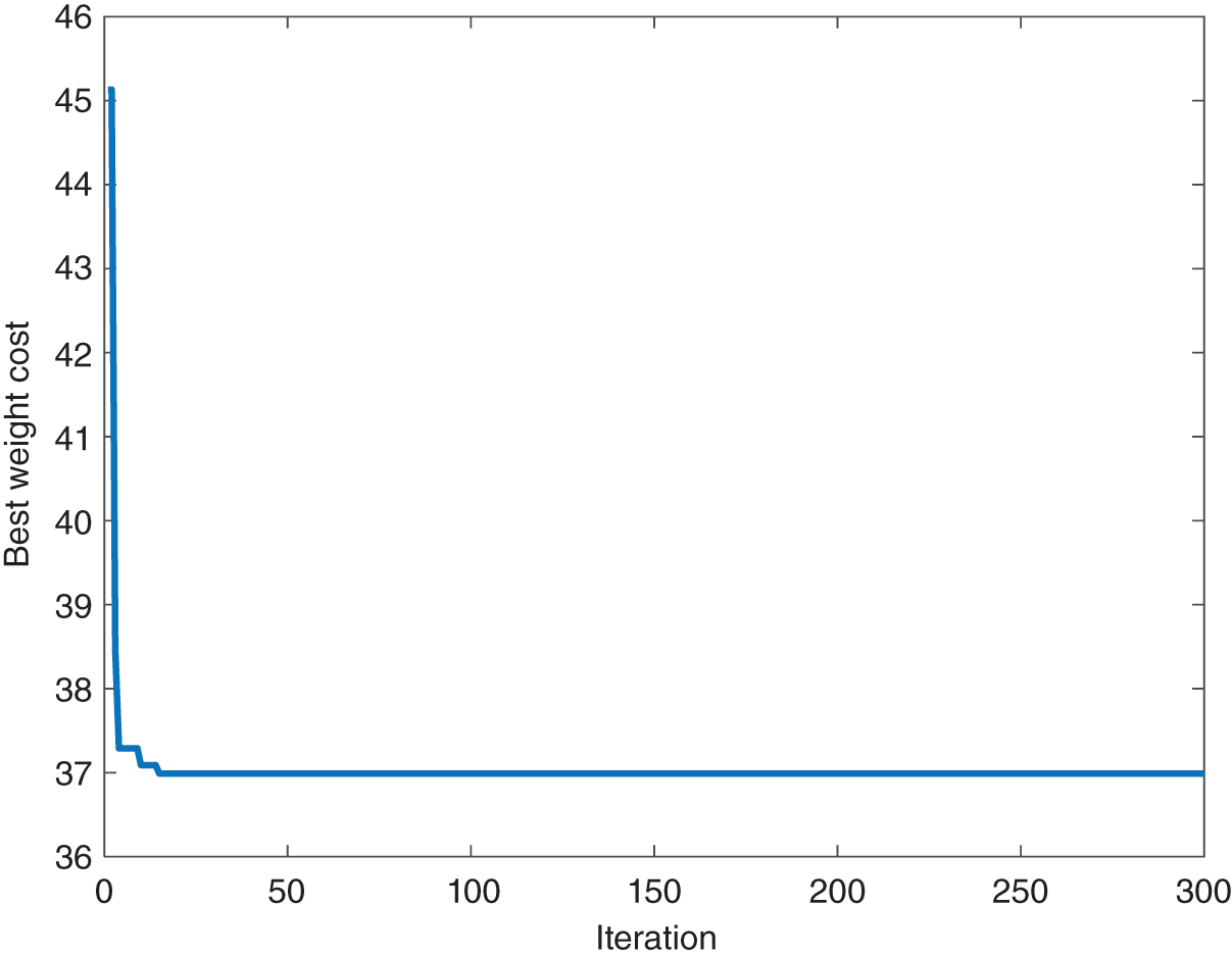
Figure 7.12 Best weight cost for AFCS architecture.
The above problem has also been solved by PSO algorithm as a single‐objective optimisation. Figure 7.12 shows the value of weight cost function using PSO algorithm which is calculated z = 36.99 kg. The PSO parameters used in this simulation are shown in Table 7.5.
The problem has previously been solved by an exact method using MATLAB Intlinprog. The parameters, particularly, c1, c2 are chosen in a way that the algorithm converge to z = 36.99 kg. Three different runs were performed and each reached the desired value. In other words, they are chosen to result in the optimal solutions already calculated by the exact method. There is a general rule for setting these two learning factors that is c1 + c2 ≤ 4. In general, having a higher value of ω, c1, and c2 causes to explore and create newer solutions, however, the lower value of which exploit the current solutions and make them better.
Table 7.5 PSO parameters for minimum weight architecture.
| Iteration | Population | ω | c1 | c2 |
|---|---|---|---|---|
| 300 | 50 | 1 | 0.3 | 0.3 |
7.6 Conclusion
A general method and tool have been developed to automate as well as optimise avionics integration architecture. The proposed avionics architecture has been assigned by the best possible avionics LRUs to achieve minimum weight architecture and mapping the selected LRUs to their installation locations while keeping the mass and volume constraints within limits.
References
- Airbus (1998). A319/A320/A321 Flight Deck and Systems Briefing for Pilots.
- Airbus (1999). A330/A340 Flight Deck and Systems Briefing for Pilots.
- Airbus (2006). A380 Flight Deck and Systems Briefing for Pilots.
- Airbus (2007). Getting to Grips with FANS (Future Air Navigation System).
- Airbus (2011). A350 Flight Deck and Systems Briefing for Pilots.
- Andersson, H. (2009). Model based systems engineeeing in avionics design and aircraft simulation. Linkoping University.
- Andersson, H. and Sundkvist, B.‐G. (2006). Method and integrated tools for efficient design of aircraft control systems. 25th International Congress of the Aeronautical Sciences.
- Annighöfer, B., Kleemann, E., and Thielecke, F. (2011). Model‐based development of integrated modular avionics architecture on aircraft level. Deutscher Luft‐ und Raumfahrtkongress.
- Annighöfer, B., Kleemann, E., and Thielecke, F. (2013). Automated selection, sizing, and mapping of integrated modular avionics modules. IEEE/AIAA 32nd Digital Avionics Systems Conference (DASC).
- Annighöfer, B., Reif, C., and Thielecke, F. (2014). Network topology optimisation for distributed integrated modular avionics. Digital Avionics Systems Conference, Colorado Springs, CO, USA.
- Annighöfer, B., Nil, C., Sebald, J., and Thielecke, F. (2015a). Structured and symmetric IMA architecture optimization: use case ARIANE launcher. 34th Digital Avionics Systems Conference (DASC).
- Annighöfer, B., Nil, Ç., Sebald, J., and F. Thielecke (2015b). ARIANE‐5‐based studies on optimal integrated modular avionics architectures for future launchers. 6th European Conference for Aeronautics and Space Sciences.
- ATR (2015). ATR 72‐600 Maintenance Training Manual.
- BAE Systems (2007). BAE 146/AVRO 146 RJ Seriess, Aircraft Flight Manual.
- Bauer, C., Lagadec, K., Bès, C., and Mongeau, M. (2007). Flight control system architecture optimisation for fly‐by‐wire airliners. J. Guidance Control Dyn. 30 (4): 1023–1029.
- Bokhari, S.H. (1987). Assignment Problems in Parallel and Distributed Computing. Norwell, MA, United States: Kluwer Academic Publishers.
- Burkard, R., Dell'Amico, M., and Martello, S. (2009). Assignment Problems. Philadelphia, USA: Society for Industrial and Applied Mathematics (SIAM).
- Butz, H. (2007). Open integrated modular avionics (IMA): state of art and future development road map at Airbus Deutschland. Workshop on Aircraft Systems Technologies (AST), Hamburg, Germany.
- Carta, D., Oliveira, J. D., and Starr, R. (2012). Allocation of avionics communication using Boolean satisfiability. 31st Digital Avionics Systems Conference.
- Cessna (2000). Cessna Citation XLS Instrumentation and Avionics.
- Charara, H., Scharbarg, J.‐L., Ermont, J., and Fraboul, C. (2006). Methods for bounding end‐to‐end delays on an AFDX network. Real‐time Systems, Euromicro Conference.
- Ching‐Lai, H. and Kwangsun, Y. (2011). Multiple Attribute Decision Making: Methods and Applications. Berlin Heidelberg: Springer‐Verlag.
- Dayama, N. R., Todi, K., Saarelainen, T., and Oulasvirta, A. (2020). GRIDS: interactive layout design with integer programming. Association for Computing Machinery, Honolulu, HI, USA.
- Delange, J., Pautet, L., and Plantec, A. (2002). Validate, simulate and implement ARINC653 systems using the AADL. Proceedings of the ACM SIGAda International Conference, New York.
- DOD (2019). Technology Readiness Assessment Guide. DOD.
- DOE (2015). Technology Readiness Assessment Guide. DOE.
- Dougherty, B., Schmidt, D., White, J., and Kegley, R. (2011). Deployment optimisation for embedded flight avionics systems. CrossTalk, Nov–Dec 2011, 31–36.
- EUROCONTROL (2017). Avionics Requirements for Civil Aircraft. EUROCONTROL.
- Feiler, P. H., Gluch, D. P., and Hudak, J. J. (2006). The architecture analysis & design language (AADL): an introduction. Carnegie Mellon University.
- Förster, S., Fischer, M., Windisch, A., and Balser, B. (2003). A new specification methodology for embedded systems based on the π‐calculus process algebra. Proceedings of the 14th IEEE International Workshop on Rapid Systems Prototyping.
- Fraboul, C. and Martin, F. (1999). Modeling advanced modular avionics architectures for early real‐time performance analysis. Proceedings of the Seventh Euromicro Workshop on Parallel and Distributed Processing.
- Galli, L. (2018). Algorithms for integer programming. IEEE.
- Gavel, H. (2007). On aircraft fuel systems conceptual design and modeling. PhD Thesis. Linkoping University.
- Guerra, C. J., Carmichael, N. E., and Nielson, J. T. (2016). Aircraft avionics strategic fleet update using optimal methods. IEEE Aerospace Conference, Big Sky, MT, USA.
- Hardung, B. (2006). Optimisation of the allocation of functions in vehicle networks. PhD thesis. Erlangen: Erlangen University.
- ICAO (2005). Annex 2, Rules of the Air, 10the. ICAO.
- ICAO (2007). ICAO Doc 4444: PANS‐ATM (Procedures for Air Navigation Services), 15the. ICAO.
- ICAO (2013). Annex 14, Aerodromes, Volume 1 Aerodrome and Operations, 6the. ICAO.
- Jackson, B. and J. Norgard (2002). A stochastic optimisation tool for determing spacecraft avionics box placement. IEEE Aerospace Conference, Big Sky, MT, USA.
- Jensen, P.A. (2002). Operation Research Models and Methods. Wiley.
- Johansson, O. and Krus, P. (2006). Configurable design matrixes for system engineering applications. The Proceeding of IDETC/CIE ASME, USA.
- Johansson, O., Andersson, H., and Krus, P. (2008). Conceptual design using generic object inheritence. Proceedings of the ASME International Design Engineering Technical Conference, New York.
- Kafil, M. and Ahmad, I. (1997). Optimal task assignment in hetrogeneous computing systems. Hetrogeneous Computing Workshop.
- Kirby, M. R. (2002). Technology identification, evaluation and selection. Aerospace Systems Design Laboratory, Georgia Institute of Technology.
- Lafaye, M., Gatti, M., Faura, D., and Pautet, L., (2011). Model driven early exploration of IMA execution platform. IEEE/AIAA 30th Digital Avionics Systems Conference, Seattle, WA, USA.
- Lauer, M. and Ermont, J. (2011). Latency and freshness analysis on IMA systems. Main Technical Program at IEEE ETFA.
- Lee, Y.‐H., Kim, D., Younis, M., and Zhou, J. (2000). Scheduling tool and algorithm for integrated modular avionics systems. 19th DASC. 19th Digital Avionics Systems Conference, Philadelphia, PA, USA.
- Lo, V. (1988). Heuristic algorithms for task assignment in distributed Systems. IEEE Trans. Comput. 37 (11): 1384–1397.
- Manolios, P., Vroon, D., and Subramanian, G. (2007). Automating component‐based system assembly. Proceedings of the 2007 International Symposium on Software Testing and Analysis.
- Minot, F. (2010). Method for optimisation of an avionics platform. US Patent No. 2010/0292969 A1, issued 18 November 2010.
- NASA (2007). NASA System Engineering Handbook NASA/SP‐2007‐6105, Rev 1. US: NASA.
- NASA (2016). Final Report of the NASA Technology Readiness Assessment (TRA) Study Team.
- Nickum, J., Robert Cormier, Albert Herndon et al. (2002). Avionics integration: a process to optimise avionics components to meet desired operational capabilities. AIAA's Aircraft Technology, Integration, and Operations (ATIO), Los Angeles, California.
- PREEvision (2020). https://www.vector.com/int/en/products/products-a-z/software/preevision/#c1789 (accessed 11 August 2021).
- Radaei, M. (2021). Mathematical programming for optimization of integrated modular avionics. SAE Technical Paper 2021‐01‐0009, 2021. https://doi.org/10.4271/2021-01-0009.
- Saaty, T. (1980). The Analytic Hierarchy Process. New York: McGraw‐Hill.
- Sabatini, R. (2000). MB‐339CD aircraft development: COTS integration in a modern avionics architecture. RTO Symposium on “Strategies to Mitigate Obsolescence in Defence Systems”, Budapest, Hungary.
- Sagaspe, L. and Bieber, P. (2007). Constraint‐based design and allocation of shared avionics resources. 26th Digital Avionics Systems Conference.
- Salomon, U. and Reichel, R. (2011). Automatic safety computation for IMA systems. IEEE/AIAA 30th Digital Avionics Systems Conference.
- Salomon, U. and Reichel, R. (2013). Automatic design of IMA systems. IEEE Aerospace Conference Proceedings.
- Salzwedel, H. and Fischer, N. (2008). Aircraft level optimisation of avionics architecture. 27th Digital Avionics Systems Conference.
- Seabridge, A. (2017). Lecture notes on avionics data networking, hardware intergration and testing. Cranfield University.
- Seabridge, A. and Moir, I. (2020). Design and Development of Aircraft Systems, 3rde. London: Wiley.
- Shi, X. and Zhang, C. (2016). Integration design tool for avionics system based on mathematical programming. IEEE/AIAA 35th Digital Avionics Systems Conference (DASC).
- Sousa, F., Louiz, R., Marconi, E., and J. Calos (2013). A tool for multidisciplinary design conception of spacecraft equipment layout. 22nd International Congress of Mechanical Engineering, Brazil.
- Triantaphyllou, E. (2000). Multi‐Criteria Decision Making Methods: A Comparative Study. Boston, MA: Springer.
- Wang, G. and Zhao, W. (2020). The Principles of Integrated Technology in Avionics Systems. London: Elsevier.
- Weilkiens, T., Lamm, J.G., Roth, S., and Walker, M. (2015). Model‐Based System Architecture. Hoboken, NJ: Wiley.
- Wolsey, L.A. and Nemhauser, G.L. (1999). Integer and Combinatorial Optimisation. Canada: Wiley.
- Yang, J., Chen, X., and Yao, W. (2016). A rectangular cuboid satellite module layouts method based on integer optimisation. 6th International Conference on Advanced Design and Manufacturing Engineering.
- Zhang, S. (2008.) Communication infrastructure supporting real‐time applications. PhD Thesis, Technical University of Hamburg.
- Zhang, C. and Xiao, J. (2013). Modelling and optimisation in distributed integrated modular avionics. 34th Digital Avionics Systems Conference.