
5
Network
So far, we have introduced the key concepts used to demarcate systems, to characterize uncertainty by probability theory, and to define data and information as the basis of cyber realities. In all the previous chapters, we have indicated that different elements under analysis are related to each other, but without explicitly defining how. This chapter introduces the basics of graph theory and network sciences, which are the disciplines providing the fundamental concepts to evaluate structured relations between different elements [1]. We will first introduce the mathematical theory of graphs, which formalizes the relation between vertices by edges. Then, we will present how graph theory is employed in other domains to evaluate particular networks where nodes are connected with each other by links. Different network topologies will be presented together with illustrative applications, for example, in transportation and epidemiology. We will also indicate the main limitations and problems of network sciences, which concern the relation between theoretical models and actual physical processes. This chapter provides only a brief overview of the field; for interested readers, the interactive book Network Science [2] is highly recommended.
5.1 Introduction
Graph theory is a field in mathematics that deals with structures using pairwise relations. The field started with the study about the Seven Bridges of Königsberg by Euler [3]. The problem is described as follows [4]:
The Seven Bridges of Königsberg is a historically notable problem in mathematics. Its negative resolution by Leonhard Euler in 1736 laid the foundations of graph theory and prefigured the idea of topology. The city of Königsberg in Prussia (now Kaliningrad, Russia) was set on both sides of the Pregel River, and included two large island – Kneiphof and Lomse – which were connected to each other, or to the two mainland portions of the city, by seven bridges. The problem was to devise a walk through the city that would cross each of those bridges once and only once. By way of specifying the logical task unambiguously, solutions involving either reaching an island or mainland bank other than via one of the bridges, or accessing any bridge without crossing to its other end are explicitly unacceptable. Euler proved that the problem has no solution. The difficulty he faced was the development of a suitable technique of analysis, and of subsequent tests that established this assertion with mathematical rigor.
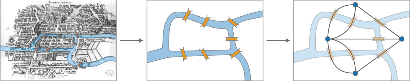
Figure 5.1 Euler's approach to prove that the problem has no solution.
Euler solved the problem by abstracting bridges and islands as edges and vertices, respectively. Figure 5.1 illustrates the problem. Euler's proof of impossibility of having a solution to the problem is considered the first result of graph theory, and network sciences [2, 5].
Graphs, as mathematical objects, are constituted by vertices that are connected by edges. For instance, the diagram on the right side in Figure 5.1 depicts the seven bridges problem as a graph composed of four vertices (circles) and linked by seven edges (black lines). This uniquely defines a specific topological structure of the graph. Note that, as a mathematical abstraction, the same graph may represent different real‐world networks. The mathematical formalism of graph theory, which is also applied by network sciences, is presented next.
In this book, we are not interested in studying graphs as pure mathematical objects but rather as networks constituted of either physical or logical relations, which will be used to understand cyber‐physical systems in the following chapters. Electric power grids and computer networks are examples of networks constituted by physical relations. Markets or social media are examples of networks constituted by logical relations.

Figure 5.2 Example of an undirected network with  nodes and
  links.
Figure 5.2 illustrates an example of an undirected network with six nodes and seven links, i.e. ![]() and
and ![]() . This graph could be a representation of connections of different university buildings, or of terminals in an airport, or researchers collaborating in papers. The first two are physical networks indicating the connections of separated buildings/terminals: building/terminal 6 is connected to building/terminal 4, which is connected to buildings/terminals 3 and 5 in addition to 6, and so on. In the last case, we have a logical network of co‐authors so that researcher 6 has a paper in collaboration with 4, who has also collaborated with 3 and 5, and so on.
. This graph could be a representation of connections of different university buildings, or of terminals in an airport, or researchers collaborating in papers. The first two are physical networks indicating the connections of separated buildings/terminals: building/terminal 6 is connected to building/terminal 4, which is connected to buildings/terminals 3 and 5 in addition to 6, and so on. In the last case, we have a logical network of co‐authors so that researcher 6 has a paper in collaboration with 4, who has also collaborated with 3 and 5, and so on.
Mathematically, this network ![]() is defined by the sets:
is defined by the sets:
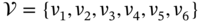 ,
, .
.
The cardinality (the number of elements) of the set ![]() is
is ![]() , and this number defines the size of the network represented by graph
, and this number defines the size of the network represented by graph ![]() . The cardinality of
. The cardinality of ![]() is
is ![]() , which indicates the number of links existing in the network. Note that networks with undirected links have, in fact,
, which indicates the number of links existing in the network. Note that networks with undirected links have, in fact, ![]() directed links; in specific cases, this must be taken into account. Sometimes, it is also possible to have edges to itself, i.e.
directed links; in specific cases, this must be taken into account. Sometimes, it is also possible to have edges to itself, i.e. ![]() .
.
Another way to mathematically represent a graph is the adjacency matrix ![]() with elements
with elements ![]() , with
, with ![]() so that
so that ![]() or
or ![]() indicating the presence or absence of a (directed) edge from vertex
indicating the presence or absence of a (directed) edge from vertex ![]() to vertex
to vertex ![]() . In our example, we have:
. In our example, we have:
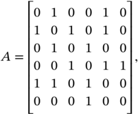
where the size of the system in ![]() . The number of edges can be computed directly from
. The number of edges can be computed directly from ![]() as:
as:
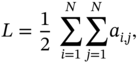
where the normalization factor ![]() is used because the network is undirected. By inspection, we can verify that
is used because the network is undirected. By inspection, we can verify that ![]() .
.
Another important concept is the degree of a node, which indicates how many links to another node it has. Mathematically, the degree of node ![]() is:
is:
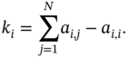
In our example, the nodes have the following degrees: ![]() ,
, ![]() ,
, ![]() ,
, ![]() ,
, ![]() , and
, and ![]() . It is also interesting to note that as the size grows, a statistical analysis of the network based on probability theory becomes relevant to characterize its structure. We will present such an approach in the next section.
. It is also interesting to note that as the size grows, a statistical analysis of the network based on probability theory becomes relevant to characterize its structure. We will present such an approach in the next section.
The links may also have some specific characteristics, such as space limitation (e.g. the capacity of the highway), the distance from one place to another (e.g. distance between the terminals in the airport), and strength of the relation (e.g. how many papers two researchers wrote together). In this case, the network is composed of weighted links. The elements of the matrix ![]() are then not only zeros and ones, but they may assume numerical values that reflect the weight of the respective link. Let us consider a modification of the matrix presented in (5.1) considering now weighted links.
are then not only zeros and ones, but they may assume numerical values that reflect the weight of the respective link. Let us consider a modification of the matrix presented in (5.1) considering now weighted links.
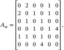
where ![]() is the adjacency matrix with weighted links.
is the adjacency matrix with weighted links.
In the case of researchers' network, this represents that researchers 4 and 6 have four papers together and researchers 1 and 2 have two; this indicates a stronger link between them. This may also indicate how many people can move from one building to another at the same time through that connection, or how far the airport terminals are.
Other important concept is the path length, which indicates how many links there are between two nodes. It is usual to have different paths connecting two nodes, and thus, their lengths also vary. The distance between two nodes is then defined as the shortest path length between them. The example presented in Figure 5.2 shows that from node 5 to node 6 there are two possible paths: ![]() , or
, or ![]() . The first has a length of two while the second four. In this case, the distance between nodes 5 and 6, denoted
. The first has a length of two while the second four. In this case, the distance between nodes 5 and 6, denoted ![]() , is given by
, is given by ![]() .
.
It is also possible to identify the number of shortest paths between two edges. In the previous case there is only one shortest path. If we now consider the paths between node 2 and node 6, we can show by inspection that there are two shortest paths, whose distance is ![]() . It is also possible to compute them directly from the adjacency matrix as presented in Chapter 2 of [2]. The diameter of the network is defined as the maximum distance between two nodes. We can prove that the diameter of the network presented in Figure 5.2 is three.
. It is also possible to compute them directly from the adjacency matrix as presented in Chapter 2 of [2]. The diameter of the network is defined as the maximum distance between two nodes. We can prove that the diameter of the network presented in Figure 5.2 is three.
There are other forms utilized to characterize networks. For example, a network is called connected if there is at least one path from any two nodes; otherwise the network is called disconnected. If all the nodes are connected to each other, we have a complete network or a clique. A component – also called cluster – is a subset of the network where at least one path from any two nodes exists. A link between two components is called bridge. The link between nodes 4 and 6 in Figure 5.2 is a bridge linking two components: one is the node 6 itself, and the component is the network formed by nodes 1, 2, 3, 4, and 5. If the bridge is broken, then the graph will become disconnected.
It is also possible to compute the cluster coefficient from any node in the network as follows:
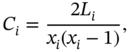
where ![]() is the number of links between the
is the number of links between the ![]() neighbors of node
neighbors of node ![]() . Note that the cluster coefficient is a number between 0 and 1 so that
. Note that the cluster coefficient is a number between 0 and 1 so that ![]() means that the neighbors of node
means that the neighbors of node ![]() are not linked to each other;
are not linked to each other; ![]() indicates that
indicates that ![]() and its neighbors form a complete graph. In our example, node 1 has
and its neighbors form a complete graph. In our example, node 1 has ![]() (two neighbors: 2 and 5) and
(two neighbors: 2 and 5) and ![]() (one link between them), then
(one link between them), then ![]() indicating that the “subnetwork” is formed by 1, 2, and 5 is complete. Node 3 has
indicating that the “subnetwork” is formed by 1, 2, and 5 is complete. Node 3 has ![]() (two neighbors: 2 and 4) and
(two neighbors: 2 and 4) and ![]() (no link between them), then
(no link between them), then ![]() indicating that 2 and 4 are not connected. Now, node 5 has
indicating that 2 and 4 are not connected. Now, node 5 has ![]() (two neighbor: 1, 2 and 4) and
(two neighbor: 1, 2 and 4) and ![]() (one link between 1 and 2), then
(one link between 1 and 2), then ![]() indicating the existence of some connections between neighbors, whose level of connectedness is measured by the clustering coefficient.
indicating the existence of some connections between neighbors, whose level of connectedness is measured by the clustering coefficient.
Table 5.1 summarizes the main characteristics of a network. This list is not exhaustive and many others exist, while new ones may also be proposed. References [1, 2, 5] provide an in‐depth analysis of networks and ways of characterizing them. An introduction to the mathematical formalism of graph theory can be found in [6]. In the next section, we will explore different types of networks.
Table 5.1 Summary of possible characteristics of a network ![]() as defined in Definition 5.1.
as defined in Definition 5.1.
| Characteristic | Meaning | Formulation |
|---|---|---|
| Size | Number of nodes | |
| Adjacency matrix | Representation of links | |
| Weighted adjacency matrix | Representation of links with weights | |
| Node degree | Number of connections a given node | |
| Number of links | How many links exist in the network | Directed: |
| Path length | Number of links from node | |
| Distance | Shortest path length between two nodes | |
| Diameter of a network | Maximum distance between two nodes of the network | |
| Connectedness | Indicate if the network is connected, or disconnected | — |
| Clique | Indicate parts of the network where all nodes are connected, and thus, form a complete graph | — |
| Cluster or component | Part of a network where there is at least one path between any two nodes | — |
| Bridge | Connection between two components | — |
| Cluster coefficient | Indication of how connected a given node |
5.2 Network Types
In the previous section, we introduced some of the main metrics to characterize networks using a simple example presented in Figure 5.2. This is actually a static graph that represents a relatively small system. Networks can be (and usually are) much larger, possibly changing over time. Think about the Internet itself, or social media applications. In this section, we will introduce different types of networks, from the simplest peer‐to‐peer network with only two elements to large random networks. Figure 5.3 presents an example of the network topologies to be discussed here.

Figure 5.3 Example of different network topologies.
5.2.1 Peer‐to‐Peer Networks
This is a topology that consists of two nodes that are connected to each other. In general, a peer‐to‐peer network with the size ![]() is composed of
is composed of ![]() links, where each node is only connected with another node. In this case, all nodes have degree one, i.e.
links, where each node is only connected with another node. In this case, all nodes have degree one, i.e. ![]() . This can be seen as an extreme case of a disconnected network. For example, the communication proposed by Shannon presented in the previous chapter with a transmitter and a receiver can be seen as a peer‐to‐peer network with
. This can be seen as an extreme case of a disconnected network. For example, the communication proposed by Shannon presented in the previous chapter with a transmitter and a receiver can be seen as a peer‐to‐peer network with ![]() with one directed link.
with one directed link.
5.2.2 One‐to‐Many, Many‐to‐One, and Star Networks
The one‐to‐many topology is a directed network where one “central” node is connected to all other nodes. If the network has size ![]() , then we can assume without loss of generality that node 1 is the central one. Because the network is directed, the degree of the node can be categorized as out‐ and in‐flows, and thus,
, then we can assume without loss of generality that node 1 is the central one. Because the network is directed, the degree of the node can be categorized as out‐ and in‐flows, and thus, ![]() and
and ![]() . For all the other nodes, we have:
. For all the other nodes, we have: ![]() and
and ![]() . The many‐to‐one topology can be understood as a mirrored version of the one‐to‐many. In this case, the central node have in‐flow links from all the other nodes. Then,
. The many‐to‐one topology can be understood as a mirrored version of the one‐to‐many. In this case, the central node have in‐flow links from all the other nodes. Then, ![]() and
and ![]() , while
, while ![]() and
and ![]() . The star network has the same topology as the one‐to‐many and the many‐to‐one but with undirected links. In this case, we have
. The star network has the same topology as the one‐to‐many and the many‐to‐one but with undirected links. In this case, we have ![]() , while
, while ![]() . In all three cases,
. In all three cases, ![]() .
.
5.2.3 Complete and Erdös–Rényi Networks
A undirected network where all nodes are connected is called complete or fully connected. In a network with size ![]() ,
, ![]() with a cluster coefficient
with a cluster coefficient ![]() . In this case there will be
. In this case there will be ![]() links in the network.
links in the network.
Erdös–Rényi (ER) networks were introduced by Hungarian mathematicians Erdös and Rényi in [7] to study random graphs with ![]() nodes, which is a fixed number. The uncertainty in this network is related to the randomness of (i) the number of links, and (ii) the connection between nodes created by these links. Extreme cases are when the network has no links (i.e. it is only a collection of disconnected points) and a complete network where all the nodes are connected.
nodes, which is a fixed number. The uncertainty in this network is related to the randomness of (i) the number of links, and (ii) the connection between nodes created by these links. Extreme cases are when the network has no links (i.e. it is only a collection of disconnected points) and a complete network where all the nodes are connected.
Without loss of generality, consider any two nodes ![]() and
and ![]() and a potential link
and a potential link ![]() between them. The existence of
between them. The existence of ![]() is associated with a random variable
is associated with a random variable ![]() with a sample space
with a sample space ![]() where
where ![]() is associated with the absence of
is associated with the absence of ![]() while
while ![]() denotes the existence of such a link. The probability mass function of
denotes the existence of such a link. The probability mass function of ![]() is
is ![]() and
and ![]() . In ER networks, the existence of a link between any two nodes in the network is determined by the outcomes of the independent outcomes of the random variable
. In ER networks, the existence of a link between any two nodes in the network is determined by the outcomes of the independent outcomes of the random variable ![]() .
.
In this case, a probabilistic characterization of the graph is possible. For example, each node in the network has ![]() links on average. If
links on average. If ![]() , the ER network is reduced to a complete graph. Likewise, if
, the ER network is reduced to a complete graph. Likewise, if ![]() , the ER network is just a collection of points. They are the aforementioned extreme cases, which are actually deterministic. Note that the ER network is completely characterized by it size
, the ER network is just a collection of points. They are the aforementioned extreme cases, which are actually deterministic. Note that the ER network is completely characterized by it size ![]() and the probability
and the probability ![]() . A formalization of ER networks is the target of Exercise 5.1. A detailed mathematical analysis of ER networks can be found in [1, 2, 5, 7].
. A formalization of ER networks is the target of Exercise 5.1. A detailed mathematical analysis of ER networks can be found in [1, 2, 5, 7].
5.2.4 Line, Ring, and Regular Networks
The line network is defined when the nodes are connected to form a line, and thus, all nodes have two neighbors except the border nodes. If its size is ![]() , then the network will have
, then the network will have ![]() links. If we assume that the border nodes are nodes 1 and
links. If we assume that the border nodes are nodes 1 and ![]() , then the node degrees are
, then the node degrees are ![]() and
and ![]() . This network is connected and the cluster coefficient is
. This network is connected and the cluster coefficient is ![]() . The diameter of the network is
. The diameter of the network is ![]() , determined by the distance between the two extremes.
, determined by the distance between the two extremes.
If the ring topology is similar but the border nodes are connected, then ![]() and
and ![]() . If
. If ![]() , then
, then ![]() . The diameter of this network considering both directed and undirected links is part of Exercise 5.2, and thus, we will not present it here.
. The diameter of this network considering both directed and undirected links is part of Exercise 5.2, and thus, we will not present it here.
Regular topologies are a broader term that usually refers to any topology that has a deterministic pattern. The already discussed line and ring topologies, as well as the star topology, can be classified as regular. Other regular grids are, for example, a rectangular, or a hexagonal grid, and also variations of the ring topology where nodes are symmetrically connected with ![]() neighbors. Regular networks are deterministic and symmetric in contrast to random networks like ER.
neighbors. Regular networks are deterministic and symmetric in contrast to random networks like ER.
5.2.5 Watts–Strogatz, Barabási–Albert and Other Networks
Watts–Strogatz (WS) networks are random graphs proposed by Watts and Strogatz in a paper published in 1998 [8]. The idea was to capture the small‐world phenomena illustrated by the famous study by Milgram [9], which indicated that, even in very large social networks, the average path lengths between nodes are small. Watts and Strogatz proposed a method to generate networks with such a characteristic starting from a variation of a ring topology where nodes are connected with ![]() neighbors. From the initial regular topology, nodes are randomly rewired with a given probability
neighbors. From the initial regular topology, nodes are randomly rewired with a given probability ![]() . In the extreme cases, the WS network is a regular grid if
. In the extreme cases, the WS network is a regular grid if ![]() , and a ER network is
, and a ER network is ![]() . The example presented by the authors is a pedagogical way to explain how a WS network can be generated [8]:
. The example presented by the authors is a pedagogical way to explain how a WS network can be generated [8]:
Random rewiring procedure for interpolating between a regular ring lattice and a random network, without altering the number of vertices or edges in the graph. We start with a ring of
vertices, each connected to its
nearest neighbors by undirected edges. (For clarity,
and
in the schematic examples shown here, but much larger
and
are used in the rest of this Letter.) We choose a vertex and the edge that connects it to its nearest neighbor in a clockwise sense. With probability
, we reconnect this edge to a vertex chosen uniformly at random over the entire ring, with duplicate edges forbidden; otherwise we leave the edge in place. We repeat this process by moving clockwise around the ring, considering each vertex in turn until one lap is completed. Next, we consider the edges that connect vertices to their second‐nearest neighbors clockwise. As before, we randomly rewire each of these edges with probability
, and continue this process, circulating around the ring and proceeding outward to more distant neighbors after each lap, until each edge in the original lattice has been considered once. (As there are
edges in the entire graph, the rewiring process stops after
laps.) Three realizations of this process are shown, for different values of
. For
, the original ring is unchanged; as
increases, the graph becomes increasingly disordered until for
, all edges are rewired randomly. One of our main results is that for intermediate values of
, the graph is a small‐world network: highly clustered like a regular graph, yet with small characteristic path length, like a random graph.
This text refers to Figure 5.4, which is adapted from the original paper.

Figure 5.4 Example of a WS network.
Source: Adapted from [8].
Barabási–Albert (BA) networks were proposed in [10] considering a scenario where new nodes are added over time by a probabilistic mechanism called preferential attachment. The idea behind this approach is that any new node has higher chances to be connected with the nodes that have higher degrees, which leads to the emergence of hubs (i.e. nodes that are highly connected).
In fact, BA networks are a particular case of scale‐free networks, defined when the degree distribution of nodes follows a power law probability distribution. Mathematically, a power law distribution is defined as ![]() with
with ![]() , being then a heavy‐tailed distribution (i.e. it is not exponentially bounded like Gaussian or Poisson distributions). Power laws have also the interesting property of scale invariance: for a given function
, being then a heavy‐tailed distribution (i.e. it is not exponentially bounded like Gaussian or Poisson distributions). Power laws have also the interesting property of scale invariance: for a given function ![]() with
with ![]() being an arbitrary constant and a scaling factor
being an arbitrary constant and a scaling factor ![]() , we have
, we have ![]() .
.
Although scale‐free networks have received attention as a tool to model real‐world interactions, recent results indicate that the scale‐free property might not be as widespread as initially thought [11]. Besides, there are several other alternatives of networks such as tree, mesh, and bus, as well as hybrid topologies or those without a specific type.
Such a structural characterization is important when describing processes that happen on networks, such as transference of data packets on the Internet, possible flight routes between two cities, or propagation of viruses. This is the focus of the next section.
5.3 Processes on Networks and Applications
So far, we have shown how to characterize the structure of networks, also including procedures used to generate random graphs through rewiring as in WS or through preferential attachment as in BA. Networks are usually related to structural components where operating and flow components exist to jointly constitute a given system. In that case, networks represent the infrastructure that supports processes that constitute a functioning system.
The following subsections exemplify three different processes on networks, namely a data communication system, transportation in cities, and virus propagation. Our aim is to show how the network topology directly affects such processes in an intuitive manner without formulating the problem using the mathematical tools of dynamical systems.
5.3.1 Communication Systems
As indicated by Shannon's model [12], the peculiar function of a communication system is to transfer data from one point in space and/or time to another. Details of communication and computer networks can be found in textbooks, such as [13, 14]; detailed historical notes can be found in [15]. Consider two persons: Amanda and Bob. Amanda is willing to tell Bob that she will take a new course on cyber‐physical systems.
If both Amanda and Bob are in the same room, she can just tell it in a peer‐to‐peer link. However, if they are in a lecture room far from each other, Amanda decides to write this on a piece of paper and send it to him through a path with two other nodes that relay the message. In this last case, the message is routed in a regular grid. If Amanda and Bob are in their own houses, Amanda decides to call Bob by a landline phone that is connected through a public switched telephone network (PSTN), which has a hierarchical tree‐like topology with levels of switching systems. Amanda could also use her connection to the Internet either by sending an instant message from her computer, or by calling Bob by a Voice over Internet Protocol (VoIP) using her mobile phone connected to a cellular network of fourth generation (4G). The Internet forms a dynamic decentralized network with hubs, which could be characterized under some conditions as scale‐free that may follow a BA network, e.g. [2].
Each real‐world situation has characteristics of its own. For example, if Amanda is telling the news to Bob in the same room, there might be more people talking, or loud music, and thus, the peer‐to‐peer link may break. In this case, the two nodes are not connected and the network stops functioning. As a consequence, we can say that the network is not robust against this missing link. The situation described in the lecture room is different: the written message can reach its final destination through several paths, not necessarily the shortest one. If a link is broken because an absent node (i.e. no one is sitting at that table to forward the message to the destination), alternative routes may still be possible. We can then say that this network has a certain level of resilience with respect to missing links, i.e. even without a few links, the function of the communication network can be accomplished. However, if certain links are absent, the network may not percolate, and thus, the message cannot reach its final destination.
We could also compare the difference of calling by using PSTN and VoIP. Without going into technical details, PSTNs are based on a dedicated hierarchical network that resembles a star topology, and thereby, with important central nodes that connect Amanda and Bob by multiple circuit switches. The robustness of the network as a whole is highly dependent on its central nodes. Once established, this link is exclusive with quality guarantees. VoIP, in its turn, runs on the Internet, which is a dynamic network‐based data multiplexing using packet switching technology, without explicit quality guarantees. VoIP “slices” the voice into smaller data packets that travel through the network in different routes to reach the address of the final destination, multiplexed with all other possible data packets (e.g. other VoIP, videos, and text files). At the destination, the packets are grouped together and decoded as voice. The quality of a VoIP call is usually worse than that of PSTN calls, but the network is more resilient because of the existence of several hubs and many possible routes.
5.3.2 Transportation in Cities
The case studied by Euler presented in Figure 5.1 can be seen as an example of how transportation networks could be modeled as a graph. This was clearly a toy example, but very illustrative because it indicates the impossibility of a solution to the Seven Bridges problem. One of the classical problems in the literature of transportation networks is the traveling salesman problem [16]. The problem is the following: Given a list of cities with their connections, what is the shortest possible route that visits each city exactly once and returns to the origin city? This problem can be formulated as a graph with weighed edges, which results in a combinatorial optimization problem; in the literature of computer sciences, this is known as a typical example of a problem that cannot be solved in polynomial time.
Without going into the details of NP‐hardness and its importance for operational research and logistics, we will focus on topological aspects of the network and how this affects transportation in cities. Consider the Berlin S‐Train map presented in Figure 5.5. Each station is a node connected by edges, which are associated with different train lines. Outer stations have a low degree while central stations high, resembling a star topology. Around the center of the network there are also lines forming a ring topology. Putting together, this hybrid topology is built to have not only one overcrowded central hub, but also a few smaller hubs where the radial lines cross with the ring. In this way, the traffic of the transportation network could be balanced between different routes.
This simple daily life example illustrates how networks are part of our lives. It is interesting to mention that studying cities through the lenses of network sciences has been a tendency for a few years. For interested readers, the reference [17] is a milestone in the field by empirically showing how different characteristics of cities scale with their size along with a formalism derived from network sciences and dynamical systems.
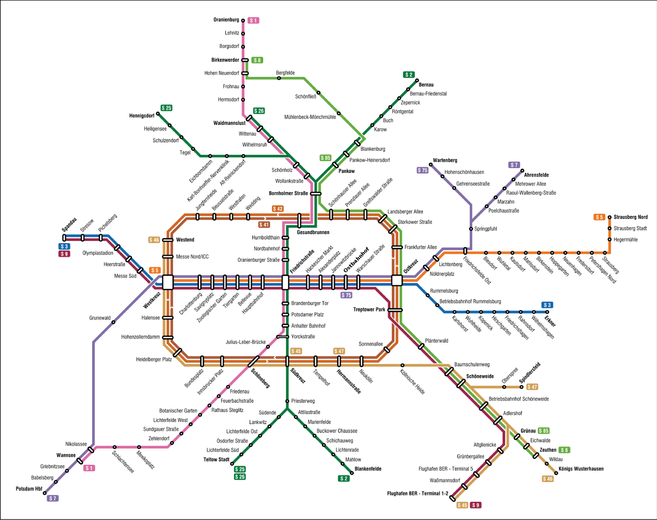
Figure 5.5 Map of the Berlin S‐Train.
Source: https://commons.wikimedia.org/wiki/File:S-Bahn_Berlin_-_Netzplan.svg.
5.3.3 Virus Propagation and Epidemiology
The COVID‐19 pandemic has led to a widespread interest in epidemiological models of how viruses and other infectious deceases propagate. In the literature there are three basic models [2], namely Susceptible‐Infected (SI), Susceptible‐Infected‐Susceptible (SIS), and Susceptible‐Infected‐Recovered (SIR). The premise employed in those models is that individuals can be classified with respect to a given pathogen as:
- Susceptible: Healthy individuals that have not yet contacted the pathogen;
- Infected: Individuals that carry the pathogen and can infect susceptible individuals if they are in contact;
- Recovered: Individuals who have been infected before, but are healthy, and thus, cannot propagate the pathogen.
Without going into the mathematical characterization based on differential equations and random walking theory, the idea of SI, SIS, and SIR basic models is to analytically assess when a disease will be spread over all population, or the effect of the spreading rate – the famous ![]() that dominated the news in 2020 during the COVID‐19 pandemic, which, in the words of Barabasi [2], is the number of new infections each infected individual causes under ideal circumstances.
that dominated the news in 2020 during the COVID‐19 pandemic, which, in the words of Barabasi [2], is the number of new infections each infected individual causes under ideal circumstances.
The SI model is the one that assumes that there is no recovery, and thus, it indicates how long a given population will be fully composed of infected individuals. The SIS model assumes that individuals can recover, but they are immune and they can become infected once again. In this case, two outcomes at the population level may happen: (i) an endemic state where there is an equilibrium so that there is always a given ratio of the population infected, or (ii) a decease‐free state where the pathogen cannot propagate and fades away from the population. The situation (i) is associated with ![]() , while (ii) with
, while (ii) with ![]() . The SIR model adds another class of individuals that are not susceptible to the pathogen and also do not transmit it. These are recovered individuals, who are immune to the pathogen after infection. In this basic SIR model, all the elements of the population will be eventually recovered. Those models could also be adapted to include immunization and individuals that died.
. The SIR model adds another class of individuals that are not susceptible to the pathogen and also do not transmit it. These are recovered individuals, who are immune to the pathogen after infection. In this basic SIR model, all the elements of the population will be eventually recovered. Those models could also be adapted to include immunization and individuals that died.
Once again, it is interesting to quote Barabasi [2]:
In summary, depending on the characteristics of a pathogen, we need different models to capture the dynamics of an epidemic outbreak. (…) [T]he predictions of the SI, SIS, and SIR models agree with each other in the early stages of an epidemic: When the number of infected individuals is small, the disease spreads freely and the number of infected individuals increases exponentially. The outcomes are different for large times: In the SI model everyone becomes infected; the SIS model either reaches an endemic state, in which a finite fraction of individuals are always infected, or the infection dies out; in the SIR model everyone recovers at the end. The reproductive number predicts the long‐term fate of an epidemic: for
the pathogen persists in the population, while for
it dies out naturally.
For this reason, we can see the importance of the ![]() factor so highly discussed during the COVID‐19 pandemic.
factor so highly discussed during the COVID‐19 pandemic.
In a seminal paper [18], Pastor‐Satorras and Vespignani expanded those basic epidemiological models from generic dynamical equations to scenarios with a networked structure. In this case, individuals are nodes in the network whose links refer to pairwise contacts between individuals. The propagation of a pathogen is actually a result of social interactions, including transportation networks in cities and daily activities, as well as international traveling and popular sports or music events. As indicated by studies of cities and transportation networks, epidemiological networks are usually associated with scaling laws, and thus, there will be some nodes with a very high degree. Such nodes are super‐spreaders. Although each pathogen is different, understanding the networked dynamics of its propagation is essential to design proper interventions to combat epidemics [2, 19].
Figure 5.6 illustrates the propagation of different flu strains using the open‐source tool called Nexttrain [20]. It is interesting to see how different strains propagate as a network connecting different regions. The granularity of this tool is not enough to capture the networked dynamics of the SI, SIS, and SIR models, but it illustrates the effects of international traveling in flu epidemics. Note that an additional aspect can be added in the model to include exposures, defined as the immediate neighbors of a given infected node. This model is known as Susceptible‐Exposed‐Infected‐Susceptible (SEIR) [21].
5.4 Limitations
Understanding networks and processes on networks is highly important. The year of 2020 serves as an illustrative example: networked models have been developed to combat the COVID‐19 pandemic and the propagation of fake news in social media. The main limitations of network sciences are related to topics already discussed in Chapter 1: the relation between a particular scientific theory and its respective object. Despite being a controversial topic, we think it is important to indicate the dangers of either data‐driven or purely mathematical models, as well as a tendency of universality that is dominant in the field.
5.4.1 From (Big) Data to Mathematical Abstractions
Big data and data‐driven approaches where “machines learn” patterns from data are widespread. As indicated by Nextstrain and [2], empirical data can be used to build mathematical models capable of predicting events such an outbreak. However, as reported in [11], modeling (big) data related to complex networks is not straightforward and may create a tendency of empirically finding scale‐free networks. Such an approach may lead to empirical scaling laws that may lead to inaccurate predictions. Besides, if the predictive model affects the dynamics of the network evolution, the mathematical abstraction may become intrinsically incorrect because of a feedback loop.
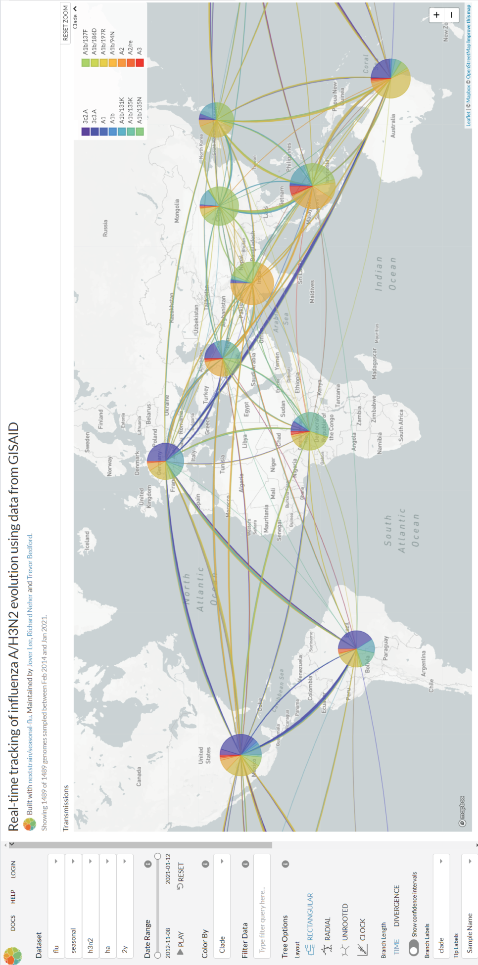
Figure 5.6 Snapshot of the spatiotemporal propagation of flu using Nextstrain. Generated through https://nextstrain.org/flu/.
5.4.2 From Mathematical Abstractions to Models of Physical Processes
Generative mathematical models that assume an ideal, purified object to characterize complex real‐world networks may also be problematic. Similar to what we have described before about empirical data being “forced” to fit the characterization of scale‐free networks, generative mathematical models for networks may likewise be misleading. For instance, predictions for COVID‐19 based on generative models can be wrong but useful as discussed in [22]. What should be highlighted is that mathematical models cannot impose itself on the reality of the process under consideration. If the data obtained from the real world network do not behave as expected by the generative model, the evaluation ought to be fair and not blame the reality for not being the ideal model. As indicated in Chapter 1, a consistent and elegant mathematical model is neither a necessary nor a sufficient condition for being a scientific theory of a given object, including networks.
5.4.3 Universality and Cross‐Domain Issues
The two limitations just presented can, in fact, be summarized in one problem: universality. This is closely related to the discussions introduced by Broido and Clauset [11] in contrast to the view that scale‐free networks are everywhere, defended by Barabasi [2]. The question was an interesting one posed by Holme [23], as a comment about such a controversy. Similar questions might be considered by the science of cities defended by Bettencourt [17] utilizing network sciences to derive the characteristics of complex urban formations.
The question is the following: are power grids, cities, epidemics, social relations, and air traffic all following a hidden pattern revealed by network sciences? This is controversial and, for the reasons stated in Chapter 1, the position taken by this book leads to a no as the answer, although the models are indeed useful if understood a tool, not as a scientific representation of reality. Note that some objects can be scientifically characterized as networks, but it is not a universal characterization. Most of the time, network sciences provides a potentially useful model, not a scientific theory of the phenomenon under investigation.
Inga Holmdahl and Caroline Buckee precisely indicate in [22] five questions about models for COVID‐19, also stating how their results should be used. Such precautionary propositions touch the key issues mentioned above by identifying two classes of models, namely data‐driven predictive models and mechanistic mathematical models. This is what they wrote:
FIVE QUESTIONS TO ASK ABOUT MODEL RESULTS
- What is the purpose and time frame of this model? For example, is it a purely statistical model intended to provide short‐term forecasts or a mechanistic model investigating future scenarios? These two types of models have different limitations.
- What are the basic model assumptions? What is being assumed about immunity and asymptomatic transmission, for example? How are contact parameters included?
- How is uncertainty being displayed? For statistical models, how are confidence intervals calculated and displayed? Uncertainty should increase as we move into the future. For mechanistic models, what parameters are being varied? Reliable modeling descriptions will usually include a table of parameter ranges – check to see whether those ranges make sense.
- If the model is fitted to data, which data are used? Models fitted to confirmed Covid‐19 cases are unlikely to be reliable. Models fitted to hospitalization or death data may be more reliable, but their reliability will depend on the setting.
- Is the model general, or does it reflect a particular context? If the latter, is the spatial scale – national, regional, or local – appropriate for the modeling questions being asked and are the assumptions relevant for the setting? Population density will play an important role in determining model appropriateness, for example, and contact‐rate parameters are likely to be context‐specific.
(…)
Unlike other scientific efforts, in which researchers continuously refine methods and collectively attempt to approach a truth about the world, epidemiologic models are often designed to help us systematically examine the implications of various assumptions about a highly nonlinear process that is hard to predict using only intuition. Models are constrained by what we know and what we assume, but used appropriately and with an understanding of these limitations, they can and should help guide us through this pandemic.
We think that the argument put forth by the authors is also valid across several other domains in general and network sciences in particular, also including the aforementioned debate about whether scale‐free networks are rare or everywhere [23].
5.5 Summary
This chapter presented an overview of the most fundamental concepts of graph theory and network sciences. The aim was to introduce the formalism used to model relations between different elements, being then material or symbolic. We presented structural characteristics of networks and also processes on networks, both illustrated by examples from our daily lives. The limitations of network models were also discussed focusing on the dangers of either data‐driven or mathematical models. Interested readers could find a good introduction to graph theory in [6]. The core concepts and methods in network sciences are presented in an interactive manner in [2]. More advanced discussions about complex networks are presented in [5]. Current debate about epidemiological models and scale‐free networks are presented in [22] and [23], respectively.
Exercises
- 5.1 Formalization of ER networks. ER networks are presented in Section 5.2.3. Consider a network with
 nodes and a probability
  that a link between two nodes exists.
- If
 represents a random variable associated with the degree of a given node, compute the probability mass function
  , i.e. the probability that a given node in the network has
  connections.
 - Compute the expected value of
 , i.e.
  .
. - Compute the variance of
 , i.e.
- Interpret such theoretical results considering two scenarios: (i)
 varies from two to infinity, and (ii)
  varies from zero to one. Write this answer with your own words supported by the mathematical findings.
- If
- 5.2 Network topologies. Consider a network with a ring topology of
 nodes with links that are unweighted and undirected. Present the results as a function of
  .
.
- Compute the degrees of the nodes.
- Present the adjacency matrix.
- Compute the network diameter.
- Compute the cluster coefficients of the nodes.
- Analyze the ring topology with
 as a communication network (i.e. how data travel to a point to another in the network) based on the node degree, the network diameter, and the cluster coefficient.
 - Consider that you are a designer who wishes to improve the communication network described in (e). Your task is to change the ring network topology by adding only one new node and an unlimited number of links connected to it. Justify your decision and identify a vulnerability of this topology.
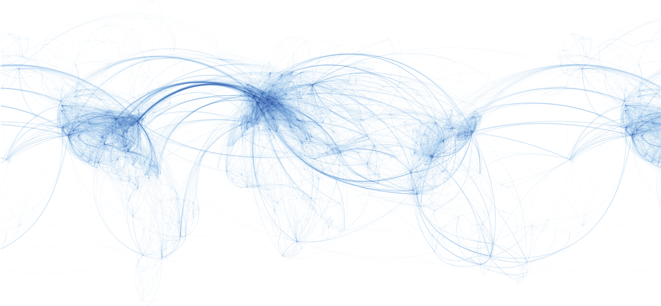
Figure 5.7 World airline routes.
Source: https://commons.wikimedia.org/wiki/File:World_airline_routes.png.
- 5.3 Networks in the real world. Consider the world airline routes presented in Figure 5.7.
- Provide a qualitative assessment of this network by, for instance, commenting about its topology and node degree distribution.
- How many clusters could you visually identify in this network?
- Consider that a new infectious disease transmitted by airborne droplet like flu appeared in the world. Which continent would be easiest to isolate? Justify.
References
- 1 Newman ME. The structure and function of complex networks. SIAM Review. 2003;45(2):167–256.
- 2 Barabási AL. Network Science. Cambridge University Press; 2016. Available online: http://networksciencebook.com/.
- 3 Euler L. The seven bridges of Königsberg. The World of Mathematics. 1956;1:573–580. Original version available online: http://eulerarchive.maa.org//docs/originals/E053.pdf.
- 4 Wikipedia. Seven Bridges of Königsberg—Wikipedia, The Free Encyclopedia; 2021. [Online; accessed 3‐February‐2021]. Available from: https://en.wikipedia.org/wiki/Seven_Bridges_of_K%C3%B6nigsberg.
- 5 Thurner S, Hanel R, Klimek P. Introduction to the Theory of Complex Systems. Oxford University Press; 2018.
- 6 Diestel R. Graph Theory. Springer; 2017.
- 7 Erdős P, Rényi A. On the evolution of random graphs. Publication of the Mathematical Institute of the Hungarian Academy of Sciences. 1960;5(1):17–60. Original version available online: https://www.renyi.hu/p_erdos/1959-11.pdf.
- 8 Watts DJ, Strogatz SH. Collective dynamics of ‘small‐world’ networks. Nature. 1998;393(6684):440–442.
- 9 Milgram S. The small world problem. Psychology Today. 1967;2(1):60–67.
- 10 Barabási AL, Albert R. Emergence of scaling in random networks. Science. 1999;286(5439):509–512.
- 11 Broido AD, Clauset A. Scale‐free networks are rare. Nature Communications. 2019;10(1):1–10.
- 12 Shannon CE. A mathematical theory of communication. The Bell System Technical Journal. 1948;27(3):379–423.
- 13 Kurose JF, Ross KW. Computer Networking: A Top‐Down Approach. Pearson; 2016.
- 14 Popovski P. Wireless Connectivity: An Intuitive and Fundamental Guide. John Wiley & Sons; 2020.
- 15 Huurdeman AA. The Worldwide History of Telecommunications. Wiley Online Library; 2003.
- 16 Flood MM. The traveling‐salesman problem. Operations Research. 1956;4(1):61–75.
- 17 Bettencourt LM. The origins of scaling in cities. Science. 2013;340(6139):1438–1441.
- 18 Pastor‐Satorras R, Vespignani A. Epidemic spreading in scale‐free networks. Physical Review Letters. 2001;86(14):3200.
- 19 Althouse BM, Wenger EA, Miller JC, Scarpino SV, Allard A, Hébert‐Dufresne L, et al. Superspreading events in the transmission dynamics of SARS‐CoV‐2: opportunities for interventions and control. PLoS Biology. 2020;18(11):e3000897.
- 20 Hadfield J, Megill C, Bell SM, Huddleston J, Potter B, Callender C, et al. Nextstrain: real‐time tracking of pathogen evolution. Bioinformatics. 2018;34(23):4121–4123. Tool available: https://nextstrain.org/.
- 21 He S, Peng Y, Sun K. SEIR modeling of the COVID‐19 and its dynamics. Nonlinear Dynamics. 2020;101(3):1667–1680.
- 22 Holmdahl I, Buckee C. Wrong but useful‐what covid‐19 epidemiologic models can and cannot tell us. New England Journal of Medicine. 2020;383(4):303–305.
- 23 Holme P. Rare and everywhere: perspectives on scale‐free networks. Nature Communications. 2019;10(1):1–3.