
Chapter 19
THE REQUIRED RATE OF RETURN
A ship in a harbour is safe but that is not what ships are built for
The previous chapter described the important concepts of risk, return and the market portfolio. It also highlighted the notion of risk premium (i.e. the difference between the return on the portfolio and the risk-free rate); this chapter continues to explore the risk premium in greater depth.
Investors must look at the big picture, first by investing in the market portfolio, then by borrowing or by investing in risk-free instruments commensurate with the level of risk they wish to assume. This approach allows them to assess an investment by merely determining the additional return and risk it adds to the market portfolio.
We now want to know how to get from r (the discounting rate used in calculating company value) to k (the return required by investors on a specific security).
Remember that this approach applies only if the investor owns a perfectly diversified portfolio.
Here is why: the greater the risk assumed by the financial investor, the higher their required rate of return. However, if they make just one investment and that turns out to be a failure, their required rate of return will matter little, as they will have lost everything.
With this in mind, it is easier to understand that the risk premium is relevant only if the financial investor manages not just a single investment, but a diversified portfolio of investments. In this case, the failure of one investment should be offset by the return achieved by other investments, which should thereby produce a suitable return for the portfolio as a whole.
This is the main difference between an industrial investment and a financial investment.
An entrepreneur who sets up their own company does not act like a financial investor, as they own just one investment. As their assets are not diversified, it is a matter of “life or death” for the firm that the investment succeeds. The law of averages in risk diversification does not apply to them.1
The financial investor, on the other hand, needs portfolio management tools to estimate the risk–return on each of their investments. Portfolio theory is not the main objective here, but it is useful to introduce some basic notions with which financial managers must be familiar.
Section 19.1 RETURN REQUIRED BY INVESTORS: THE CAPM
The CAPM (capital asset pricing model) was developed in the late 1950s and 1960s. Based on the work of Harry Markowitz, William Sharpe, John Lintner and Jack Treynor, it is now universally applied.
The CAPM is based on the assumption that investors act rationally and have at their disposal all relevant information on financial securities (see “efficient markets” in Chapter 15). Like the investor in Chapter 18, they seek to maximise their return, at a given level of risk.
The capital market line that we described in the previous chapter set the relationship for the return of a portfolio. CAPM aims at defining the same relationship but for a specific security (and not for a portfolio) in order to determine the return required for this security depending on its risk.
Remember that in order to minimise total risk, investors seek to reduce that component which can be reduced, i.e. the specific risk. They do so by diversifying their portfolios.
It can be observed that diversification reduces specific risk fairly quickly.
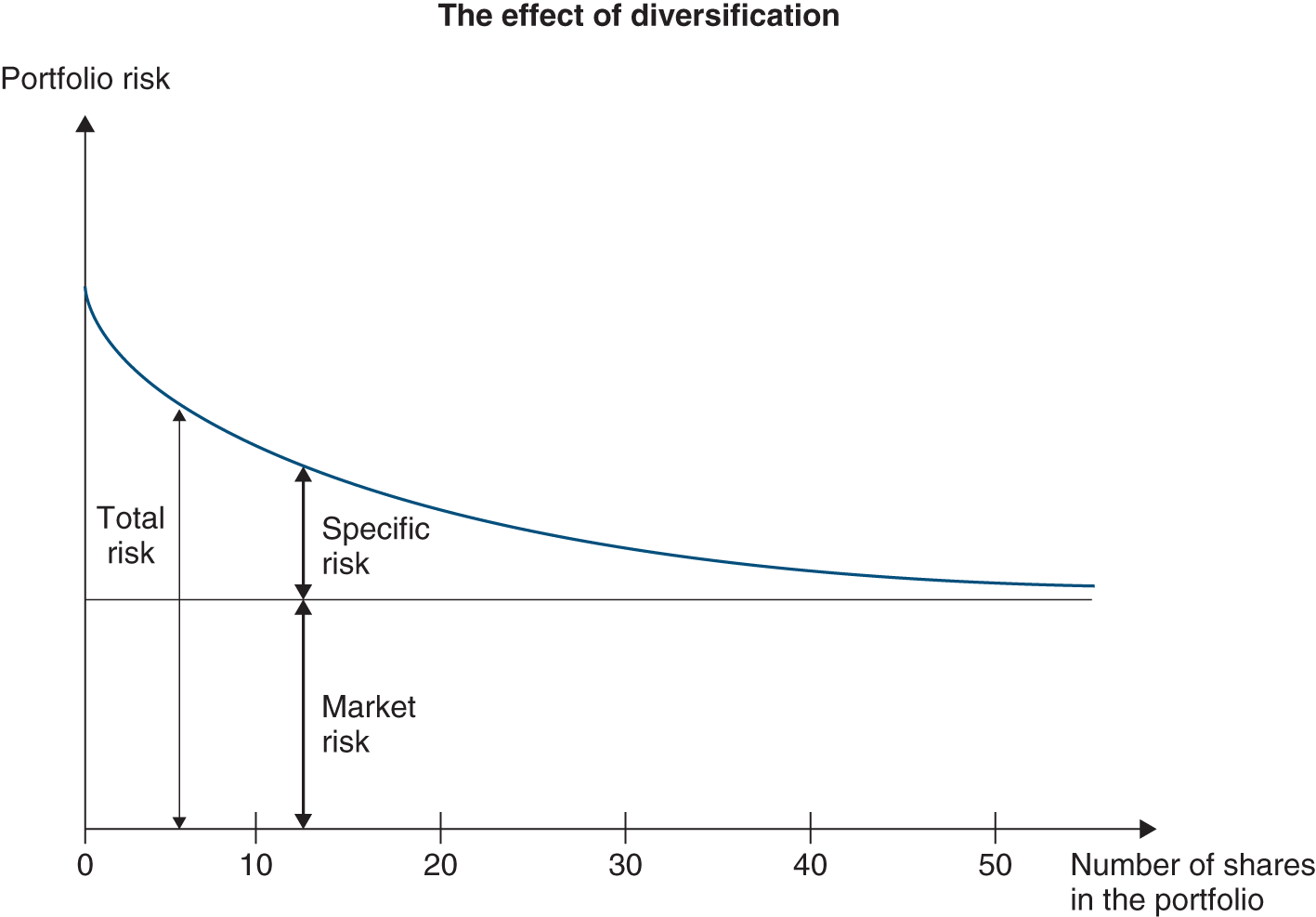
As a result, when stocks are fairly valued, investors will receive a return only on the portion of risk that they cannot eliminate – the market risk, or the non-diversifiable risk. Indeed, in a market in which arbitrage is theoretically possible, they will not be amply remunerated for a risk that they could otherwise eliminate themselves by simply diversifying their portfolios.
This means that the required rate of return (k) is equal to the risk-free rate rF,2 plus the risk premium for the non-diversifiable risk, i.e. the market risk.
This can be expressed as follows:
where kM is the required rate of return for the market and β the sensitivity coefficient described previously.
Note that the coefficient β measures the non-diversifiable risk of an asset and not its total risk. So it is possible to have a stock that is, on the whole, highly risky but with a low β if it is only loosely correlated with the market.
The difference between the return expected on the market as a whole and the risk-free rate is called the equity risk premium.
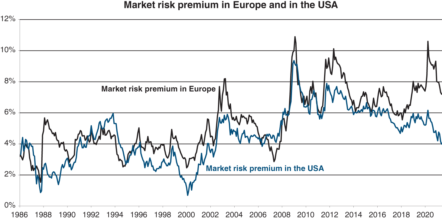
Source: Data from Associés en Finance (Europe), BNP Paribas Arbitrage & Damodaran (USA)
Over the very long term (120 years!), the historical risk premium has been as follows:
| Belgium | 3.0% | South Africa | 6.0% |
| China (1993–2020) | 4.6% | Spain | 3.3% |
| France | 5.5% | Switzerland | 3.9% |
| Germany (exc. 1922/23) | 6.2% | US | 5.8% |
| Italy | 5.6% | UK | 4.3% |
| India | 6.1% | Europe | 3.5% |
| Japan | 6.1% | World | 4.4% |
| Russia (1995–2020) | 7.4% |
Source: Crédit Suisse Global Investment Returns Yearbook, 2021. Equity risk premium compared to short-term interest rates.
The equity risk premium can be historical or expected (or anticipated). The historical risk premium is equal to the annual performance of equity markets (including dividends) minus the risk-free rate. The expected risk premium is not directly observable. However, it can be calculated by estimating the future cash flows of all the companies, and then finding the discount rate that equates those cash flows with current share prices, from which we deduct the risk-free interest rate. This expected risk premium is the one used in the CAPM.
To determine the risk premium for each stock, simply multiply the market risk premium by the stock's beta coefficient.
Hence, if the risk-free rate is –0.5% and the expected risk premium is 8.0%, a shareholder in the French car subcontractor Valeo will expect a return of –0.5% + 1.56 × 8.00% = 12.0%, if Valeo's β is 1.56, while a shareholder in L'Oreal will expect –0.5% + 0.70 × 8.0% = 5.1%, as L'Oreal's β is 0.70.
Section 19.2 THE SECURITY MARKET LINE
The research house Associés en Finance publishes the securities market line3 for the entire eurozone. It is calculated on the basis of the expected return on the y-axis and the beta coefficient of each stock on the x-axis.
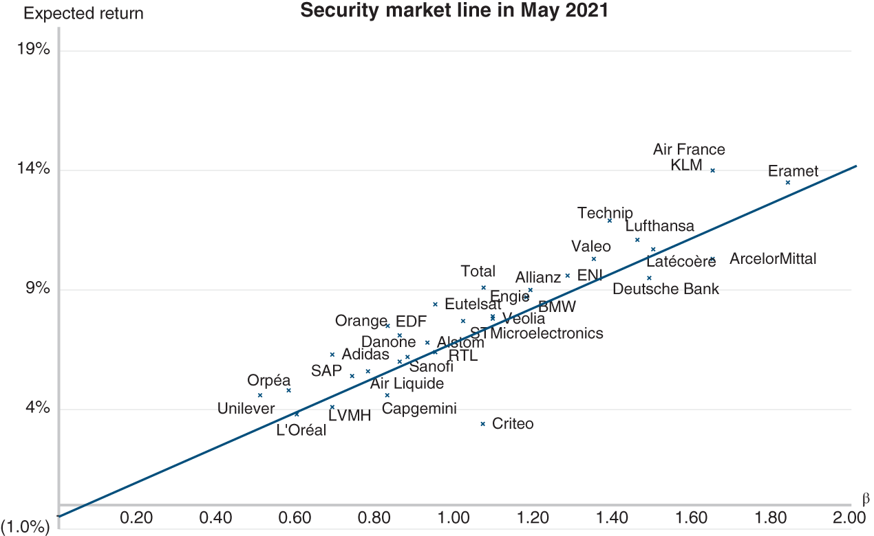
Source: Data from Associés en Finance, 2021
The securities market line is quite instructive. It helps determine the required rate of return on a security on the basis of the only risk that is remunerated, i.e. the market risk.
Shifts in the securities market line itself characterise the nature of changes in the markets and make it easier to understand them:
- a parallel shift, with no variation in slope (which represents the equity risk premium), reflects a change in interest rates. For example, a cut in interest rates normally leads to a downward shift and thus a general appreciation of all stocks;
- a non-parallel shift (or pivoting) reflects a change in the risk premium and thus in the remuneration of risk. In this case, the riskiest stocks will move the most, whereas the least risky stocks may not be significantly affected.
In addition, the position of points vis-à-vis the market line serves as a decision-making tool. The above chart tells us that Orange offers too high an expected return for its risk. Investors will realise this and buy it, thus raising its price and lowering expected return. A stock that is “above” the securities market line is thus undervalued, while a stock that is “below” the securities market line (like Adidas) is overvalued.
But do not rush to place an order. Since this chart was printed, prices have had plenty of time to adjust.
Section 19.3 LIMITS OF THE CAPM
The CAPM assumes that markets are efficient and it is without a doubt the most widely used model in modern finance. But if we wanted to be facetious, we would say that each element of the CAPM poses a practical problem!
1/ THE LIMITS OF DIVERSIFICATION
The CAPM is a development of portfolio theory and is based on the assumption that diversification helps to reduce risk reducing it to the non-diversifiable risk. A study by Campbell et al. (2001) shows that diversification is increasingly complex and that nowadays a portfolio of at least 50 stocks is required to reduce risk significantly.
This is due, among other things, to the greater volatility of individual stocks, although markets as a whole are no more volatile. Other reasons for this phenomenon are the arrival on the market of riskier companies, such as biotech, Internet and younger companies, and the near extinction of conglomerates, which, by nature, provided some diversification in and of themselves.
Meanwhile, the correlation between market return and return on individual stocks is falling. This may undermine the relevancy of the CAPM. Statistically, beta is becoming less and less relevant.
2/ DIFFICULTIES IN PRACTICAL APPLICATION OF THE CAPM
The first difficulty one encounters when using the CAPM is determining the risk-free rate which, all things considered, is just a theoretical concept.
Practitioners usually use as a risk-free rate the yield of long-term government bonds. They put forward the similar weighted average duration of the cash flows of the assets to be valued and of long-term bonds. The issue is that long-term government bonds are not without risk: their value can fluctuate in time depending on changes in interest rates (which is inevitable given the long period of time since their issue). Even investors that plan to keep government bonds until their maturity suffer from these interest rate fluctuations for the reinvestment of coupons. In addition, unanticipated changes in inflation can impact what could have appeared as a risk-free investment. Finally, there remains the solvency risk of the issuer. The increasing levels of debt of most Western countries mean that this risk is not just theoretical, as demonstrated in recent years in Greece.
Therefore, it appears more rational to use as a risk-free rate the short-term interest rate. Short-term bills are virtually not impacted by changes in interest, coupon reinvestment risk does not exist and bankruptcy risk is minor. For the Eurozone, the risk-free rate could be assessed on the basis of the return on short-term German Treasury bills.
The three key global providers of equity market risk premium data (Ibbotson, Dimson-Marsh-Staunton and Associés en Finance) propose a computation of the market risk premium based on long-term interest rates or short-term interest rates. The most important factor is not to add a short-term interest rate to a market premium computed on the basis of long-term rates, or the reverse.
Roll (1997) has pointed out that determining a market portfolio is not as easy as one would like to think. In theory, the market portfolio is not solely made up of stocks or even just financial assets, but of all the assets that can be acquired. It is therefore impossible, in practice, to come up with a true market portfolio, especially when looking at it from an international point of view.
However, we still have to determine the return expected from the market portfolio. As the CAPM is used for making forecasts, it can also be used to calculate the return expected from a security based upon the return expected from the market portfolio, as well as the security's anticipated risk (its β). However, “anticipated” data cannot be observed directly in the market, and so forecasts must be made on the basis of historical data and macroeconomic data. For some countries, such as emerging nations, this is not easy!
3/ THE INSTABILITY OF β
The main criticism of beta is its instability over time. It boils down a large amount of information into a single figure, and this strength becomes its weakness.
The CAPM is used to make forecasts. It can be used to calculate expected return on the basis of anticipated risk. Therefore, it would be better to use a forecast β rather than a historical value, especially when the coefficient is not stable over time.
For this reason, calculations must often be adjusted to reflect the regularity of earnings and dividends, and visibility on the sector. Blume et al. (1975) have sought to demonstrate a convergence of β towards 1. This seems counterintuitive to us as some sectors will always have a beta greater than 1. In addition, the recent crisis has demonstrated that, in difficult times, the gap between high β and low β increases.
4/ THE THEORETICAL LIMITS OF CAPM AND MARKETS AT FAIR VALUE
The CAPM assumes markets are fairly valued. But markets are not necessarily always at fair value. The fact that technical analysis has become so prominent on trading floors shows that market operators themselves have doubts about market efficiency (see Chapter 18).
Moreover, the theory of efficient markets in general, and the CAPM in particular, is based on the premise that market operators have rational expectations. To be applicable, the model must be accepted by everyone as being universally correct. The development of parallel theories shows that this is not necessarily the case.
The bias mentioned above has led the CAPM to be considered as just one theoretical explanation for the functioning of the financial markets. Other theories and methods have been developed, but they have not (yet?) achieved the attractiveness of the CAPM, due to the simplicity of its concepts. We should not lose hope: a study by Ferguson and Shockley (2003) posits that all weaknesses of the CAPM could be attributable to a mis-estimation of the market portfolio and that they would disappear if not only stocks, but also bonds (and other investment opportunities), were included, as the theory suggests.
Section 19.4 MULTIFACTOR MODELS
1/ THE ARBITRAGE PRICING THEORY
In some ways the APT (arbitrage pricing theory) model is an extended version of the CAPM. The CAPM assumes that the return on a security is a function of its market risk and therefore depends on a single factor: market prices. The APT model, as proposed by Stephen Ross, assumes that the risk premium is a function of several variables, not just one, i.e. macroeconomic variables (V1, V2,…, Vn) as well as company “noise”.
So, for security J:
The model does not define which V factors are to be used. Ross's original article uses the following factors, which are based on quantitative analyses: inflation, manufacturing output, risk premium and yield curve.
Comparing the APT model to the market portfolio, we can see that APT has replaced the notion (hard to measure in practice) of return expected by the market with a series of variables which, unfortunately, must still be determined. This is why APT is a portfolio management tool and not a tool for valuing stocks.
2/ THE FAMA–FRENCH MODEL
There are offshoots from the APT that have sought to explain historical returns by company-specific factors rather than the general macroeconomic factors in the APT.
For example, Eugene Fama and Kenneth French (1992) have isolated three factors: market return (as in the CAPM), price/book value (see Chapter 31) and the gap in returns between large caps and small caps (which lends credence to the notion of a liquidity effect).
Other factors can be added to this list, including P/E, market capitalisation, yield and even past performance (which is a direct contradiction of efficient market theory). However, these are based on purely empirical approaches, not theoretical ones. While they criticise the CAPM, they offer no better alternative model.
3/ LIQUIDITY PREMIUM, SIZE PREMIUM AND INVESTOR PROTECTION
Among the factors used in determining risk, the criteria by which liquidity can be measured (size, free float, transaction volumes, bid–ask spread) are often statistically significant. In other words, the required return on a security often appears to be a function of liquidity.
Hamon and Jacquillat (1999) have demonstrated the existence of a liquidity premium in Europe, which is nil for large caps and significant for small caps. The liquidity premium should be added to the return derived from the CAPM to arrive at the total return expected by the shareholder. Hamon and Jacquillat use the term “market plane” (instead of securities market line). Under their model, expected return on a security is a linear equation with two parameters: the market premium and the liquidity premium. Let us report the definition from the original article:
In May 2020, Associés en Finance estimated the market plane parameters for eurozone stocks at:
The liquidity premium, which is expected in addition to the required rate of return, finds its opposite number in the notion of “liquidity discount”.
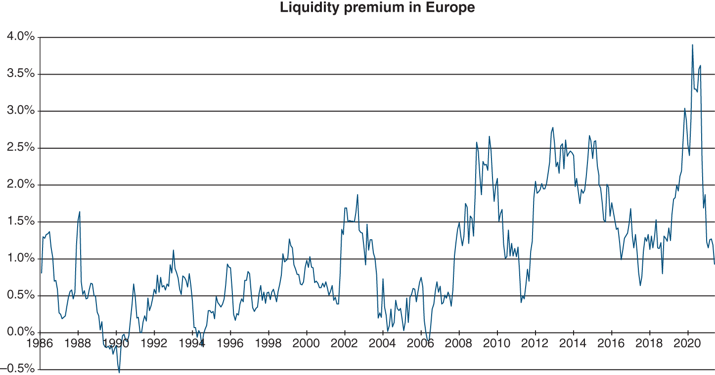
Source: Data from Associés en Finance
Section 19.5 FRACTALS AND OTHER LEADS
The theory of a market in equilibrium is based on the assumption that prices have reached an equilibrium. It therefore assumes that there is an equilibrium between offer and demand and that it is reached at every moment on financial markets (thanks to the arbitrage principle). From this equilibrium, no one can predict how prices will move: they follow a random path.
Some research proposes that market prices do not follow random paths as the market in equilibrium theory predicts. In particular, extreme events (strong price growth or large drops) occur much more frequently than would be predicted by classical theory.
Several theories have been developed to model the evolution of prices and allow for possible massive price movements (in particular, crashes).
Some have tried to use chaotic functions to model prices. Chaotic here does not mean illogical or random. The term is used for perfectly predictable series of data that appear to be illogical. These models are used in a number of sciences, including economics.
Mandelbrot has put forward that fractals (or to be more precise, multi-fractals) could provide accurate representations of market price movements. This assumption does not fit with the efficient market theory, not only because the statistical rule for modelling prices is different, but more importantly because Mandelbrot's assumptions imply that prices have memory, i.e. that they are not independent from past prices.
Section 19.6 TERM STRUCTURE OF INTEREST RATES
Because it is a single-period model, the CAPM draws no distinction between short-term and long-term interest rates. As has been discussed, a money-market fund does not offer the same annual rate of return as a 10-year bond. An entire body of financial research is devoted to understanding movements in interest rates and, in particular, how different maturities are linked. This is the study of how the yield curve, which at a point in time relates the yield to maturity to the maturity (or duration) of bonds, is formed.
1/ THE VARIOUS YIELD CURVES
By charting the interest rate for the same categories of risk at all maturities, the investor obtains the yield curve that reflects the anticipation of all financial market operators.
The concept of premium helps explain why the interest rate of any financial asset is generally proportional to its maturity.
Generally speaking, the yield curve reflects the market's anticipation regarding:
- long-term inflation;
- the central bank's monetary policy; and
- the issuing country's debt management policy.
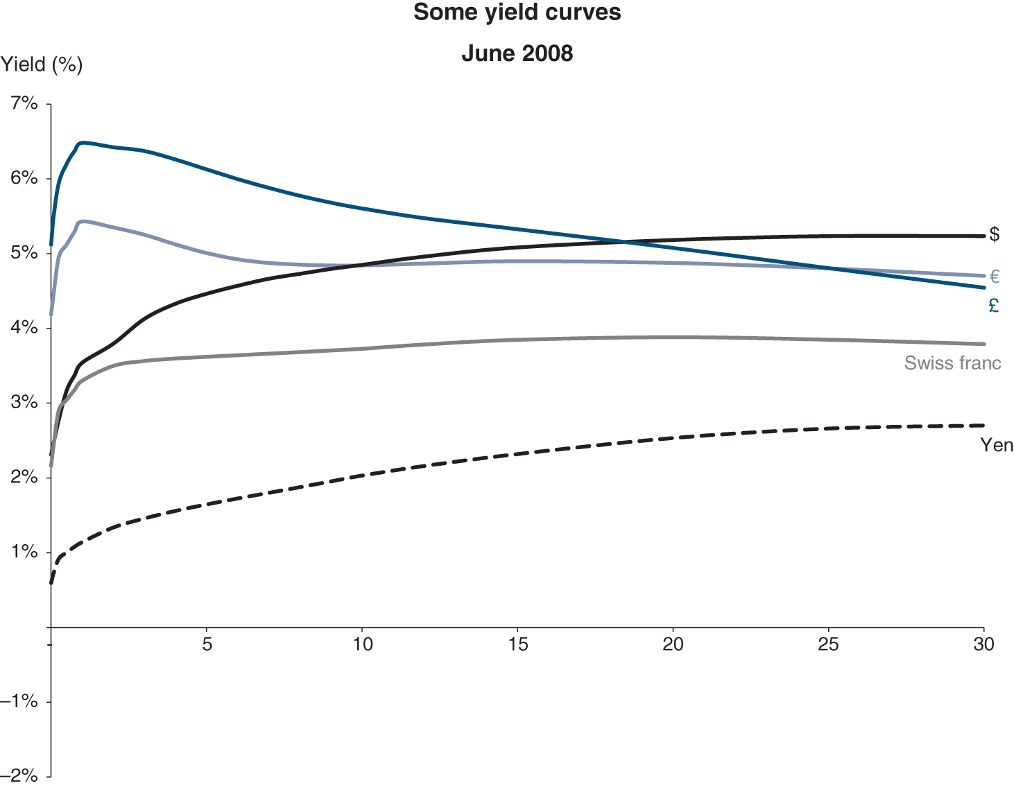
Source: Data from Datastream, Bloomberg
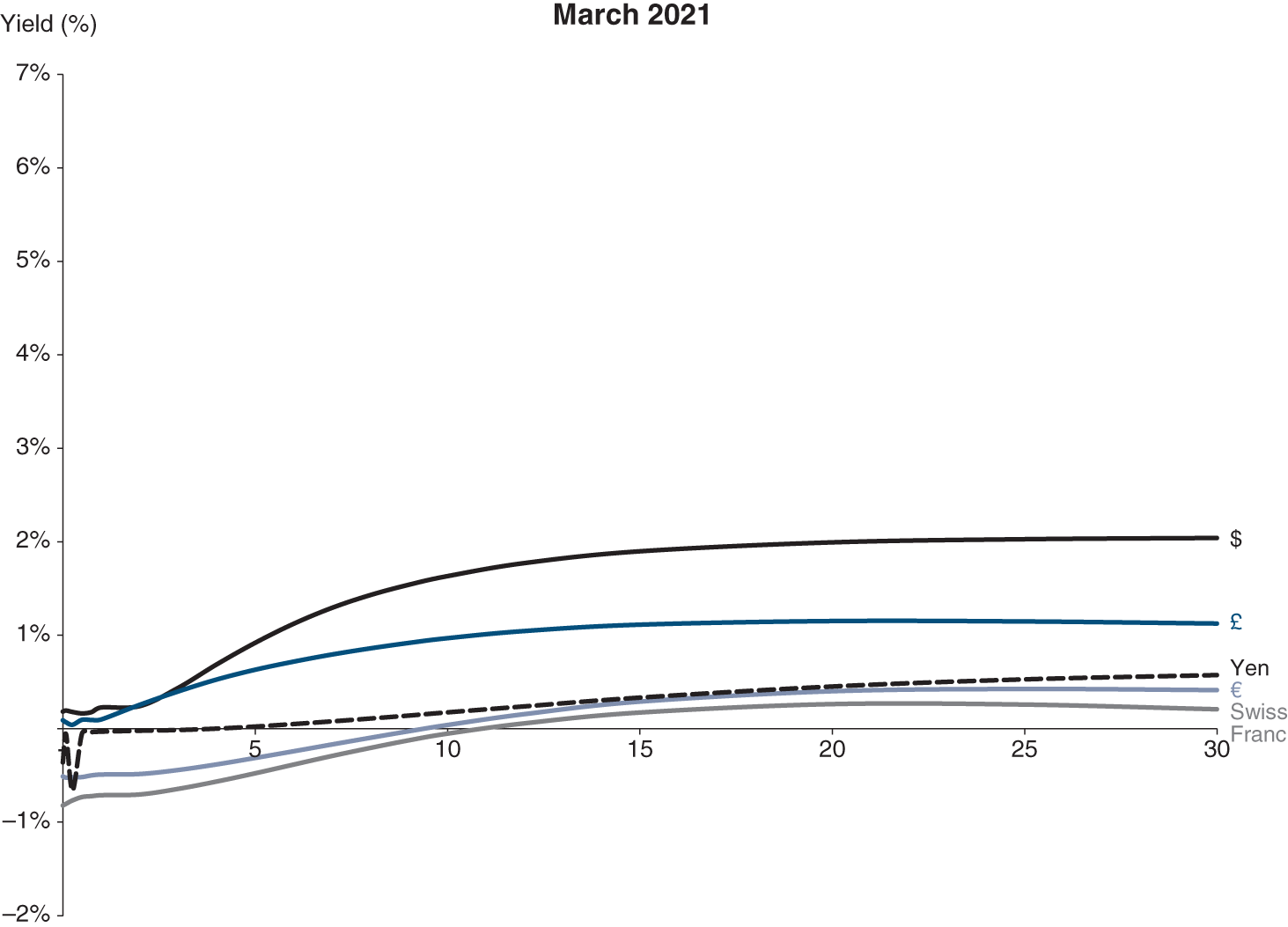
Source: Data from Bloomberg
Hence, during a period of economic recovery, the yield curve tends to be “normal” (i.e. long yields are higher than short yields). The steepness of the slope depends on:
- how strong an expected recovery is;
- what expectations the market has about the risk of inflation; and
- the extent to which the market expects a rapid increase in central banks' intervention rates (to calm inflationary risks).
For the euro, the curve's upward slope in 2021 is due to the extremely low (currently negative) levels reached by short-term rates, following European Central Bank (ECB) interventions to avoid a major economic downturn and to support the economy.
In contrast, when a recession follows a period of growth, the yield curve tends to reverse itself (with long-term rates falling below short-term rates). The steepness of the negative slope depends on:
- how strong expectations of recovery are;
- how credible the central bank's policy is (i.e. how firm the central banks are in fighting inflation); and
- the extent to which inflationary trends appear to be diminishing (despite the recession, if inflationary trends are very strong then long-term rates will tend to remain stable, and the curve could actually be flat for some time).
This is what could be observed at the beginning of 2021 in relation to the dollar.
Lastly, when rates are low, the curve cannot remain flat for any length of time because investors will buy fixed-rate bonds. As long as investors expect that their capital gain, which is tied to falling long-term rates, is more than the cost of short-term financing, they will continue to purchase fixed-rate bonds. However, when long-term rates seem to have reached a lower limit, these expectations will disappear because investors will demand a differential between long-term and short-term rates' yield on their investment. This results in:
- either a rebound in long-term rates; or
- stable long-term rates if short-term rates fall because of central bank policies; and
- a steepening in the curve, the degree of which will depend on the currency.
We then revert to the upward slope since the end of 2008 for the Swiss franc.
2/ RELATIONSHIP BETWEEN INTEREST RATES AND MATURITIES
By no means are short-term and long-term rates completely disconnected. In fact, there is a fundamental and direct link between them.
About 20 years ago, this relationship was less apparent and common consensus favoured the theory of segmentation, which said that supply and demand balanced out across markets, with no connection among them, i.e. the long-term bond market and the short-term bond market.
As seen above, this theory is generally no longer valid, even though each investor will tend to focus on their own timeframe. It is worthwhile reviewing the basic mechanisms. For example, an investor who wishes to invest on a two-year time basis has two options:
- invest for two years at today's fixed rate, which is the interest rate for any two-year investment; or
- invest the funds for one year, is paid the one-year interest rate at the end of the year, and then repeat the process.
In a risk-free environment, these two investments would produce the same return, as the investor would already know the return that they would be offered on the market in one year for a one-year bond. As they also know the current one-year rate, they can determine the return on a two-year zero-coupon bond.
where 0r2 is the current two-year rate, 1r1 the one-year rate in one year and 0r1 the current one-year rate.
Hence:
If today the one-year interest rate is 3% and the two-year interest rate is 4%, this means that the market expects the one-year interest rate to reach 5% in one year, as
An increase in short-term rates is then anticipated by the market.
In such a world, the shape of the yield curve provides some valuable information. For example, if long-term rates are higher than short-term rates, this necessarily implies that investors are anticipating an increase in interest rates.
This theory assumes that investors are not sensitive to risk and therefore that there is no preference for a short-term or a long-term investment. This does not deal with the attention that investors pay to liquidity, as demonstrated by recent events on financial markets.
3/ TAKING LIQUIDITY INTO CONSIDERATION
The first theories to highlight the existence of a premium to reflect the relative lack of liquidity of long-term investments were the preferred habitat theory and the liquidity preference theory.
In the mid-1960s, Modigliani and Sutch advanced the theory of preferred habitat, which says that investors prefer certain investment timeframes. Companies that wish to issue securities whose timeframe is considered undesirable will thus have to pay a premium to attract investors.
The theory of liquidity preference is based on the same assumption, but goes further in assuming that the preferred habitat of all investors is the short term. Investors preferring liquidity will require a liquidity premium if they are to invest for the long term.
Even if investors anticipate fixed short-term rates, the yield curve will slope upward due to the liquidity premiums.
4/ YIELD CURVES AND VALUATION OF SECURITIES
After having studied the yield curve, it is easier to understand that the discounting of all the cash flows from a fixed-income security at a single rate, regardless of the period when they are paid, is an oversimplification, although this is the method that will be used throughout this text for stocks and capital expenditure. It would be wrong to use it for bonds.
In order to be more rigorous, it is necessary to discount each flow with the interest rate of the yield curve corresponding to its maturity: the one-year rate for next year's income stream, the three-year rate for flows paid in three years, etc. Ultimately, yield to maturity is similar to an average of these different rates.
SUMMARY
QUESTIONS
EXERCISES
ANSWERS
BIBLIOGRAPHY
NOTES
- 1 However, the very fact that the entrepreneur does not diversify their portfolio means that they must achieve strong performances in managing their company, as they have everything to lose. So they are likely to take steps to reduce risk.
- 2 For the risk-free rate, kF is equal to rF. The required rate of return is equal to the return that is actually received, as the asset has no risk.
- 3 It differs from the capital market line, which has the total risks of the security on the x-axis, not the β coefficient.