
CHAPTER 6
Pricing Biases and SOFR Curve Building
A prerequisite for a successful transition from LIBOR to SOFR is that market participants are able to construct a term structure of SOFR interest rates extending years into the future, making it possible to price SOFR loans, swaps, swaptions, caps, and similar instruments tied to SOFR rates over time. And given their relative liquidity, SOFR futures are an integral component in the construction of a SOFR term structure. In fact, for now, SOFR futures are often the only set of instruments used to construct a yield curve for the SOFR complex.
Market participants familiar with the LIBOR complex will be familiar with the key role that Eurodollar futures prices have played in the construction of LIBOR curves. And as part of that experience, they're likely to be familiar with the convexity bias attributed to Eurodollar futures. In particular, every quant worth his salt learns to adjust the prices of Eurodollar futures for this bias before using these prices as inputs to his LIBOR curve-building algorithm.
So before delving into the minutiae of SOFR yield curves, we'll consider whether SOFR futures might suffer from any similar biases that would require adjustment before using their prices to construct a SOFR term structure. And as a first step in that process, we'll review the situation for Eurodollar futures.
BIASES IN EURODOLLAR FUTURES PRICES
When considering potential biases afflicting SOFR futures prices, it's useful to remind ourselves of the biases present in their predecessor, the Eurodollar futures contract. These days, most academics and industry quants use the term convexity bias to refer to the difference between a Eurodollar futures rate and the forward LIBOR rate that covers the same period, often as embedded within a forward rate agreement. But this wasn't always the case.
The seminal paper on the difference between futures rates and forward rates is The Relation Between Forward Prices and Futures Prices, written by John Cox, Jonathan Ingersoll, and Stephen Ross, and published in the Journal of Financial Economics way back in 1981. Professors Cox, Ingersoll, and Ross (CIR) compared the relative prices of two contracts for forward settlement: a plain vanilla forward contract, and a futures contract. The only difference between the two was that the futures contract was subject to continuous margining while the forward contract was not.
In the event the futures price was positively correlated with the short-term interest rate paid on margin, the person who was long this contract would find that there was a tendency for him to earn a greater interest rate precisely when the balance in his margin account was greater and to earn a lower interest rate when the balance in his margin account was lower. Likewise, the person who was short this contract would find that there was a tendency for him to earn a lesser interest rate precisely when the balance in his margin account was greater and to earn a greater interest rate only when the balance in his margin account was relatively small.
Being averse to free lunches, people selling futures contracts require higher selling prices in exchange for being on the losing end of this proposition. And people buying futures contracts are willing to pay more for their positions, given their expectation that they'll be on the winning end of the proposition.
Note that we'd expect the situation to be reversed in the event the correlation between the futures price and the short-term interest rate were negative. In that case, the person holding the short position in the futures contract would find that he was benefiting from relatively greater interest rates precisely when the balance of his margin account was high, and he'd find that he was experiencing low interest rates precisely when the value of his margin account was low. Again, the person who was long this contract would experience the opposite effect. With the holder of the short position benefiting and the holder of the long position suffering, the two parties would be expected to transact at a relatively lower price than they would otherwise, to account for this effect.
One of the most important propositions in the CIR paper is that, if the short-term interest rate paid on margin is nonstochastic, then the futures price and the forward price should be equal. This would be the case trivially in the event that the interest rate was constant – or that there was no interest paid on margin at all.
More generally, if there were no correlation between the futures price and the short-term interest rate paid on margin, then the futures price and the forward price should be equal. This is trivially the case when the interest rate is nonstochastic.
The Eurodollar futures price is defined as 100 less the Eurodollar futures rate. And since the Eurodollar futures rate is positively correlated with the short-term interest rate paid on margin, the correlation between the Eurodollar futures price and the short-term interest rate is negative. And, following Cox, Ingersoll, and Ross (1981), we'd expect the futures price in that case to be lower than it would be otherwise, as a result of this financing effect. And with the futures price lower than it would be otherwise, we'd expect the futures rate to be greater than it would be otherwise.
Note that at no point in this argument did the concept of convexity make an appearance. These results are entirely motivated by the financing of profit and loss via the margining of the futures contract. And in the industry, that's precisely the term that was used to describe this effect – the financing bias. If the futures price is negatively correlated with the short-term interest rate, then the financing bias exists to balance the inherent advantage of the person who is short the futures contract.
In this case, how does convexity enter the picture?
NONLINEARITIES RESULTING FROM CONTRACT DEFINITIONS
Let's compare two instruments that derive their values from the same segment of a yield curve. And to abstract from extraneous issues, let's maintain the assumption that we're dealing with a riskless curve. In fact, we can assume that we're dealing with the SOFR curve. Finally, let's assume for the moment that there is no interest paid on margin, in which case the financing bias is equal to zero.
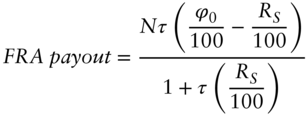
The first instrument will be a forward rate agreement (FRA), with the usual convention that the present value of the difference between RS, the spot rate at time ![]() (the expiration of the FRA), and ϕ0, the FRA rate agreed at time 0, will be paid at time S. More specifically:
(the expiration of the FRA), and ϕ0, the FRA rate agreed at time 0, will be paid at time S. More specifically:
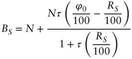
This payout is meant to hedge the interest earned on the deposit, N, made at time S and held until time ![]() . Adding this payout to the deposit of N (and simplifying), we see that the amount we have in our bank account at time S is given by
. Adding this payout to the deposit of N (and simplifying), we see that the amount we have in our bank account at time S is given by
The value of ϕ0 is negotiated at time 0 so that the value at time 0 of the random FRA payout is equal to 0.
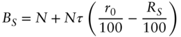
From this, the balance of our bank account at time T can be obtained by investing BS at the rate RS from time S to time T. Simplifying this, we have
From this equation, we see that ϕ0 does indeed play the role of a forward rate, despite being paid at time S rather than time T – the reason being that it's the present value of ![]() that is paid at time S.
that is paid at time S.
The second instrument we'll consider will be styled after the Eurodollar futures contract – the only difference being that the final settlement price of the futures contract in this example will be ![]() , where RS is the term rate at time S for lending from time S to time T. Again, we assume that no interest is paid on margin balances.
, where RS is the term rate at time S for lending from time S to time T. Again, we assume that no interest is paid on margin balances.
The payout of this Eurodollar-style contract at time S is given by

For example, if N is equal to USD 1 million and ![]() , then this payout is USD 25 per basis point difference between the futures rate, r0, and the term rate at settlement, RS, as is the case with the actual Eurodollar futures contract.
, then this payout is USD 25 per basis point difference between the futures rate, r0, and the term rate at settlement, RS, as is the case with the actual Eurodollar futures contract.
If we add this payout at time S to our cash investment of N at time S, we see that the balance of our bank account at time S will be
The balance of our account at time T can be determined by investing BS at term rate RS for the term ![]() . In this case (and with some algebra), we have
. In this case (and with some algebra), we have
The first term in this equation, ![]() , is the amount we would want to have in our bank account at time T if r0 were the forward rate at time 0 for lending from time S to time T.
, is the amount we would want to have in our bank account at time T if r0 were the forward rate at time 0 for lending from time S to time T.
The second and third terms, ![]() , show the effect at time T of having the futures payout at futures expiry, time S, rather than at the end of the lending period, time T.
, show the effect at time T of having the futures payout at futures expiry, time S, rather than at the end of the lending period, time T.
Figure 6.1 shows the all-in interest earned on the one-million-dollar deposit made at time S with the futures hedge and with the FRA hedge. In each case, the USD 1 million is invested at the prevailing term rate, RS, along with the time S proceeds of the hedge, from time S to time T.
There are a few points worth noting.
- The interest earned via the FRA hedge is not a function of RS, the term rate at time S, because the payout at time S (the end date of the FRA and the settlement date of the futures contract) is the present value of the difference between the FRA rate and the term rate RS (scaled by Nτ). As a result, this is simply a constant (of USD 5,000 in this case, as the FRA rate was set to 2% in this example).
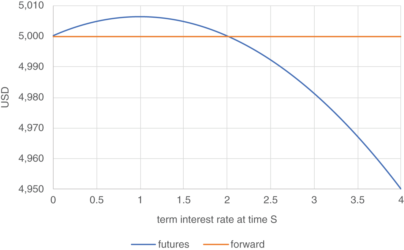
FIGURE 6.1 Time T values of all-in interest earned via futures and FRA hedges
Source: Authors
- The interest earned via the futures hedge is a function of RS, because the payout of the futures hedge gets reinvested at the rate RS between times S and T.
- Consistent with the formulae above, the interest earned through time T via the futures hedge is a strictly concave function of RS. In fact, it's a parabola – i.e., it's quadratic in RS.
We know from Jensen's inequality that the expected value of a concave function, g(x), is less than or equal to the value of the function evaluated at the expected value of x. In algebraic terms, if g(x) is a concave function of x, then
Equality obtains in the event the standard deviation of x is zero.
Furthermore, the expected value of a concave function of g(x) is a decreasing function of the standard deviation of x.
With this in mind, let's consider what that means for our concave function of RS, shown in Figure 6.1.
First, the role of the market is to find a value for the futures rate so that the expectation of the value of the all-in interest as of time T is equal to the certain interest obtained in conjunction with the FRA hedge. When this futures rate is increased, this parabola shifts higher, increasing the expected value of the parabola, ceteris paribus. When the futures rate is decreased, the parabola shifts lower, decreasing the expected value of the parabola.
Second, the expected value of the parabola is a decreasing function of the standard deviation of RS. When the standard deviation of RS is large, the parabola needs to be higher than it would be in the event that the standard deviation of RS is small.
The standard deviation of RS is a function of two things. One is the amount of time that interest rates have been able to change since the trade was initiated at time 0. In particular, the standard deviation of RS will be an increasing function of S (assuming the trade was initiated at time 0).
The other thing that affects the standard deviation of RS is the volatility of rates generally and of RS in particular. If rates are volatile, the standard deviation of RS will be greater than it would be if volatility is low.
Taken together, all this implies that the required adjustment for nonlinearity is an increasing function of the time until the futures contract expires and an increasing function of the volatility of interest rates, everything else equal. (And as a reminder, we're still abstracting from the financing bias by assuming that no interest is paid on margin.)
From all this, we take away two main points:
- There is a financing bias to consider, even when the contract in question is a simple, linear function of the interest rate underlying the contract. For example, if two counterparties decide to subject an FRA to standard futures-style margining, the FRA rate will be subject to a financing bias as well, assuming of course that the underlying FRA rate is correlated with the short-term interest rate paid on margin.
- Even if we control for a financing bias (e.g., by considering a case in which there is no interest paid on margin), there is a nonlinearity involved when comparing an FRA rate with a Eurodollar futures rate. Because we compared the two rates at the end of the lending period they cover, the nonlinearity appeared to us in the form of the value of the futures payout being a concave function of the settlement rate, RS.
Of course, the goal of this book is to understand SOFR futures rather than Eurodollar futures, so we won't go into any further detail concerning Eurodollar futures. (There's a considerable literature on this subject available for readers who would like to learn more.) But on the other hand, many people who approach the issue of biases in SOFR futures will attempt to apply their understanding of Eurodollar futures as a default template, so it's useful to review the issues here.
BIASES IN SOFR FUTURES
From the discussion of Eurodollar futures, we see there are two questions we should be asking about biases in SOFR futures.
- Are SOFR futures prices subject to any biases due to nonlinearities?
- Are SOFR future prices subject to a financing bias?
We'll see that the answer to the first question is no in the case of the three-month SOFR contract but yes in the case of the one-month contract. And we'll see that the answer to the second question is yes, probably.
Nonlinearities in the SOFR Futures Complex
The time T payout of a three-month SOFR futures contract is given by
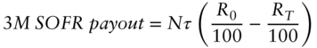
where
- R0 is the futures rate when the contract was purchased at time 0.
- RT is the settlement rate computed by compounding the daily SOFR values during the reference period.
and where N and τ are defined to be USD 1 million and 0.25 years respectively.
In addition to this payout from the futures contract, a person investing funds from time S to time T at the daily overnight SOFR values will see his balance grow from N to ![]() . Adding this balance to the funds obtained at time T via the futures hedge, we see that the combined value of his bank account at time T is given by
. Adding this balance to the funds obtained at time T via the futures hedge, we see that the combined value of his bank account at time T is given by

From which we see that R0 indeed plays the role of a forward rate for the three-month SOFR futures contract. There is no nonlinearity involved that might require us to make an adjustment to the price of the contract before using it to construct a yield curve.
Unfortunately, the situation is not as straightforward when dealing with the one-month SOFR futures contract. In that case, the time T payout to the futures contract is given by
where
- γ0 is the 1M futures rate when the contract was purchased at time 0.
- γT is the settlement rate computed by averaging the daily SOFR values during the reference period.
Again, N and τ are defined to be USD 1 million and 0.25 years, respectively.
Again, a person investing funds from time S to time T at the daily overnight SOFR values will see his balance grow from N to ![]() , where
, where ![]() is the standard rate compounded during the one-month reference period:
is the standard rate compounded during the one-month reference period:
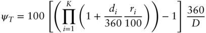
where
- K is the number of business days in the one-month reference period.
- di is the number of business days associated with the ith deposit.
- ri is the SOFR value for the ith business day.
- D is the number of calendar days in the reference period.
Combining the funds earned via overnight lending and the funds received via the futures hedge, the total time T value of the account is
We can write this expression in the form
The second term on the right-hand side, ![]() , is a function of the difference between the actual futures settlement rate, γT, which is an arithmetic average of overnight SOFR values, and
, is a function of the difference between the actual futures settlement rate, γT, which is an arithmetic average of overnight SOFR values, and ![]() , which is the futures settlement rate that would prevail in the event the one-month futures contract was settled the way the three-month futures contract was settled – i.e., with daily compounding rather than arithmetic averaging. In other words, if the one-month contract were settled the way the three-month contract was settled, the futures rate would be the forward rate corresponding to the one-month reference period. No adjustments would be required – at least no adjustments for nonlinearity. We'll get to questions of financing bias shortly.
, which is the futures settlement rate that would prevail in the event the one-month futures contract was settled the way the three-month futures contract was settled – i.e., with daily compounding rather than arithmetic averaging. In other words, if the one-month contract were settled the way the three-month contract was settled, the futures rate would be the forward rate corresponding to the one-month reference period. No adjustments would be required – at least no adjustments for nonlinearity. We'll get to questions of financing bias shortly.
What Can We Say about This Adjustment Without Making Use of a Specific Term Structure Model?
First, the daily compounded rate will be greater than the arithmetic average rate. To see this, we calculate the first derivative of the settlement futures rate as a function of each SOFR rate contained in the reference period. The first derivative of the settlement rate, RT, with respect to one day's SOFR rate, rk, is given by the expression

when using the simple arithmetic average, as in the case of the one-month contract. When using daily compounding, as per the three-month contract, the expression is
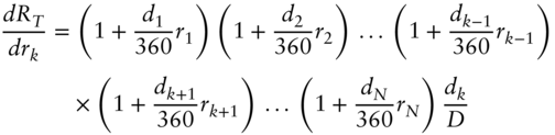
If all the rates are positive, then all the first derivatives are greater in the case of daily compounding. And if all the first derivatives are greater, then the settlement rate must also be greater. This result holds even in the case in which some of the SOFR values are zero, as long as none of the SOFR values are negative. (In the case in which all SOFR values are zero, the two settlement rates also will be zero.)
On the other hand, the difference between the rate calculated via daily compounding and the rate calculated via simple averaging is often quite small. Given the low levels of SOFR prevailing recently, the difference tends to be no more than a tenth of a basis point – and often less than that.
The differences do tend to increase with the level of simulated rates. For example, for simulated rate levels approaching 5%, the difference appears on the order of 1 basis point.
So our advice is to be aware of the issue and to use good judgment. If the purpose of the analysis requires a great deal of precision, we'd suggest running a simulation. If conditions are such that the difference appears to be of a magnitude similar to the bid–ask spread for the one-month contracts, we'd suggest making the adjustment.
The Financing Bias for SOFR Futures
If any futures contract is going to exhibit a correlation between the price of the contract and the interest rate paid on margin, the SOFR futures contract is it. In this case, the correlation between futures prices and the short-term interest rate is negative, so that the futures price should be less than it would be without the financing bias. And since the futures rate is 100 less the futures prices, the futures rate would be greater than it would be otherwise.
In theory, the bias could amount to quite a few basis points, especially when the correlation between the futures price and the short rate is high and when futures prices are volatile.
In general, the correlation with the overnight short rate is greater for shorter-dated futures at the front end of the curve than for longer-dated futures toward the back end. On the other hand, the financing effect has longer to operate when dealing with longer-dated futures, which would be expected to increase the influence of the financing bias.
Typically, quants calculate the required adjustments for each contract along the curve in accordance with the term structure model they're using to price other derivatives – an approach we recommend for the sake of consistency if nothing else. We won't go into those details here, except to note again the difficulty of identifying a term structure model that does a good job of capturing the dynamics of the SOFR term structure (including for the pricing of options on SOFR futures).
But we would like to raise two issues that may be relevant. First, the financing bias refers primarily to the effects of applying futures-style margining to an instrument. When the price of the instrument is correlated with the interest rate paid on margin, continual margining can add or subtract from the profits that otherwise would be earned on a trade. But most products these days are subject to margining, including FRAs, swaps, swaptions, caps, and floors. So if a futures contract and an otherwise similar FRA are both subject to futures-style margining, with interest paid on margin, it may not be critical to invest much time and effort making the adjustments, as the two products may well be adjusted by similar amounts.
Second, the effects of paying interest on margin only matter if the people whose trades are moving the markets are receiving interest in their margin accounts and if that interest is making it into their P&L accounts. As an anecdote, one of us (Doug Huggins) spent a number of years working as a proprietary trader at a bank and two hedge funds. At no time did anyone ever identify the interest paid or received on margin, for futures contracts or for anything else. There were times when the trades on the desk were of reasonable size (e.g., 10,000 Eurodollar butterfly spreads, involving 40,000 contracts, controlling a notional value of USD 40 billion). And we pored over every basis point along the curve. But we never included a financing bias in the analysis, because as far as we were concerned on the proprietary trading desk, we weren't paying or receiving any interest on margin. Someone clearly was, but it wasn't us. And as a result, we weren't interested in paying for something that didn't hit our P&L.
We don't know whether this experience was unusual – but it was the same in all three cases. So from our perspective, the size of the financing bias in any complex, including the SOFR complex, is probably best viewed as an empirical matter rather than as a theoretical matter. And if you believe market pricing incorporates a material financing bias, and you don't have margin interest incorporated in your P&L, then you have an opportunity to get paid for subjecting yourself to a bias that doesn't affect you. That's worth knowing, too.
BUILDING A SOFR SWAP CURVE FROM SOFR FUTURES
The discussion so far in this chapter has been somewhat academic. Let's see how these concepts can be put into practice in a real-world application – building a SOFR swap curve from a set of SOFR futures prices. In particular, we'll focus on three ways in which the construction of SOFR curves probably should differ from the construction of LIBOR curves.
Bootstrapping vs. Fitting
When building LIBOR curves, it's not unusual for people to choose as inputs a set of highly liquid instruments that cover nonoverlapping reference dates, with the result that it's possible for all input prices to be priced without error along a bootstrapped curve. Each instrument adds unique information about a specific portion of the curve, with the result that it's impossible for any of the input instruments to be arbitraged against one another.
When building SOFR curves, the basic building blocks tend to be steps delineated by FOMC meeting dates. There tend to be more of these meeting dates throughout the course of a year than are required to reprice the four three-month SOFR futures that cover the year. But there aren't enough FOMC meetings to reprice exactly all of the one-month futures contracts that cover the year. As a result, we tend to use a collection of one-month and three-month contracts when building a SOFR curve. And in this case, there certainly are more futures contracts to reprice than there are steps in the piecewise step function that defines the term structure of overnight forward rates. As a result, building SOFR curves tends to be an exercise in fitting a curve rather than bootstrapping a curve.
Price Adjustments
As already discussed, the prices of 3M SOFR futures contracts don't require any adjustments for nonlinearities, but they may require adjustment for a financing bias. The prices of one-month SOFR contracts in theory require adjustments for both issues. Again, we'd be a bit circumspect when making these adjustments. As noted above, the adjustments apparently required for the fact that the one-month contracts settle to an arithmetic average rather than via daily compounding amount to well under a basis point at the current low levels of rates. And the extent of the practical adjustment required for a financing bias is not as clear as for the theoretical adjustment, owing to the fact that there may be more than a few institutional market participants who don't feel the need to take a financing bias into account.
Discontinuities
When building LIBOR curves, we tend to avoid sharp discontinuities in forward rates, as the basic building block in a LIBOR curve tends to be the three-month rate, which changes only slowly when crossing a fixed date, such as the turn of the year, or an FOMC meeting date.
But the basic building block in a SOFR curve is the overnight rate, and it's natural to reflect sharp discontinuities, such as FOMC meeting dates, when constructing these curves.
An example should prove illustrative.
Example
Consider the construction of a SOFR curve given the settlement prices for one-month and three-month SOFR futures contracts on Friday, 25-Feb-22, shown in Table 6.1.
TABLE 6.1 SOFR futures prices as of 25-Feb-22
Source: CME
| One-month SOFR futures | Three-month SOFR Futures | |||
|---|---|---|---|---|
| Expiration Month | Settlement Price | Expiration Month | Settlement Price | |
| Jan-22 | 99.95 | Dec-21 | 99.9475 | |
| Feb-22 | 99.8 | Mar-22 | 99.4975 | |
| Mar-22 | 99.635 | Jun-22 | 99.02 | |
| Apr-22 | 99.37 | Sep-22 | 98.635 | |
| May-22 | 99.225 | Dec-22 | 98.345 | |
| Jun-22 | 99.095 | Mar-23 | 98.095 | |
| Jul-22 | 98.935 | Jun-23 | 97.95 | |
| Aug-22 | 98.875 | Sep-23 | 97.91 | |
| Sep-22 | 98.735 | Dec-23 | 97.92 | |
| Oct-22 | 98.585 | Mar-24 | 97.995 | |
| Nov-22 | 98.475 | Jun-24 | 98.06 | |
| Dec-22 | 98.395 | |||
| Jan-23 | 98.3 | |||
In this example, we choose to model the term structure of overnight forward rates as a step function, with the discontinuities corresponding to FOMC meeting dates. Our task is to assign values to the overnight forward rates in each of these steps.
As of 25-Feb, there are only a few days left in the month of February, and we can use the settlement price of the Feb22 one-month contract to bootstrap the overnight forward rate for this period. The fitted value we obtain this way is 0.0525%.
The next FOMC date is scheduled for March 16, so we can use the value of the Mar22 one-month SOFR contract to identify the height of the step beginning on March 17. In this case, we obtain a value of 0.35733%.
The following FOMC meeting isn't scheduled until 4-May-22, so that the entirety of the Apr22 contract falls within the step defined by the two FOMC dates. So at this point we have a couple of choices.
If we want to continue with the bootstrap procedure, we can either skip the Apr22 contract, as we've already used the Mar22 contract to bootstrap the value of this part of the yield curve. Or we could use the Apr22 contract to determine the height of this part of the yield curve. In this case, the value of the overnight forward rates in this part of the curve would be 0.365%, slightly greater than the value we obtained using the Mar22 one-month contract.
Our other choice would be to give up bootstrapping and to switch to calculating a fitted curve, in which we minimize the sum of squared differences between observed prices and fitted prices, with no guarantee that we'll exactly reprice any of the futures contracts with zero error. For example, if we wanted to calculate a value for this part of the yield curve by minimizing the sum of squared pricing errors for the Mar22 and Apr22 contracts, our fitted value would be 0.36355% – a bit higher than the value we calculated via the bootstrap procedure using the Mar22 price, and a bit lower than the value we calculated using the Apr22 price.
For the sake of discussion, let's assume for now that we choose to stick with the bootstrap procedure, using the Apr22 contract rather than the Mar22 contract. As a result, the value we assign to the curve between the 16-Mar-22 and 4-May-22 FOMC dates is 0.365%.
In this case, the next segment of the yield curve we need to calculate is the segment between the 4-May-22 and 15-Jun-22 FOMC dates. We can bootstrap this value using the May22 futures contract; the figure we calculate in this case is 0.65574%.
The next value we need to calculate is the value of the overnight forward rates between the 15-Jun-22 FOMC meeting date and the 27-Jul-22 meeting date. We can use the price of the Jun22 one-month contract to bootstrap this figure. In particular, the value we calculate is 0.89426%.
The next value we need to estimate is the value of the overnight forward rates between the 27-Jul-22 and the 21-Sep-22 FOMC meeting dates. In theory, we could use the value of the Jul22 one-month contract for this purpose, but as there are so few calendar days in July after the 27th, we'll use the Aug22 contract for this purpose. In this case, we estimate a value of 1.00005%.
The next value we need to calculate is the value of the overnight forward rates between the 21-Sep-22 and 2-Nov-22 FOMC meeting dates. As the entirety of the Oct22 SOFR contract is within this interval, we'll use that contract to bootstrap this part of the curve. In particular, we obtain a value of 1.18833%. It's worth mentioning that the pricing error of the Sep22 one-month contract – which we skipped in our bootstrap procedure – is nearly seven cents – quite large relative to the pricing errors we've seen so far in this example.
And speaking of pricing errors, now that we've used the prices of one-month SOFR futures contracts to bootstrap a curve out to 2-Nov-22, we can check the pricing errors of the Mar22 and Jun22 three-month contracts. In particular, the fitted price of the Mar22 contract is 0.96 cents greater than the observed settlement price, while the fitted price of the Jun22 three-month contract is 1.75 cents greater than the observed settlement price.
For reference, at this point in our bootstrapping example, the average absolute pricing error of the first nine one-month SOFR futures contracts is 0.83 cents. And the average absolute pricing error of the Mar22 and Jun22 three-month futures contracts is 1.36 cents. The largest pricing error among the one-month contacts is 6.82 cents for the Oct22 contract.
If we priced the same part of the curve using the same futures contracts by minimizing the sum of squared differences between the observed prices and the fitted prices, then the average absolute pricing error for the first nine one-month SOFR futures contracts would be 1.10 cents, and the average absolute pricing error for the Mar22 and Jun22 three-month contracts would be 0.50 cents. The largest pricing error among the one-month contracts would be 4.44 cents for the Sep22 contract. The largest pricing error between the Mar22 and Jun22 three-month contracts would be 0.65 cents for the Mar22 contract.
It's not surprising that the prices of the one-month futures were, on average, more accurately priced using the bootstrap approach, as many of these one-month contracts were the contracts that were being bootstrapped. But even in this case, the maximum pricing error among the first nine one-month contracts was lower under the fitted procedure than it was under the bootstrap procedure. And the results for the Mar22 and Jun22 three-month futures contracts were uniformly better, as would be expected given that their prices weren't used in the bootstrap but were reflected in the fitted curve exercise.
Ultimately, the choice between bootstrapping a curve and fitting a curve depends on the application. If there are certain futures contracts for which the calculated prices absolutely must equal the observed market prices, then bootstrapping a curve with these futures providing inputs sounds like the best approach. On the other hand, if it's not critical to precisely reprice the values of certain futures contracts, we'd probably suggest fitting a curve – i.e., choosing values for the heights of the steps in the yield curve so as to minimize the sum of squared differences between calculated prices and observed market prices.
With this in mind, we apply the fitted approach to the yield curve out to the end of 2025. The resulting pricing errors for the one-month contracts are shown in Figure 6.2.
Note that the pricing errors are quite small for the first few contracts, for which the liquidity is relatively good.
The pricing errors for the three-month contracts are shown in Figure 6.3.
Note that the difference between market prices and calculated prices are almost nil starting with the sixth three-month contract, as there were no liquid one-month futures to include in this part of the curve. Otherwise, the first few three-month futures contracts along the curve were priced with very little error, while the fourth and fifth contracts, Sep22 and Dec22, had slightly larger pricing errors, consistent with the lower levels of liquidity in these contracts.
Figure 6.4 shows the piecewise step function that represents our fitted yield curve in this case.
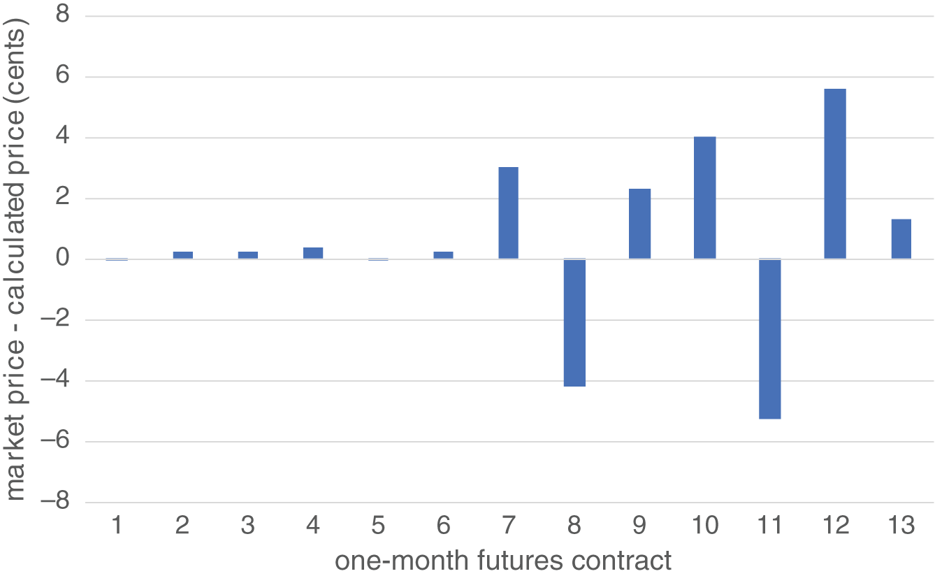
FIGURE 6.2 Fitted curve pricing errors for first 13 one-month SOFR futures contracts
Source: Authors
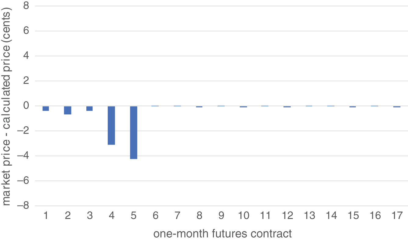
FIGURE 6.3 Fitted curve pricing errors for first 17 three-month SOFR futures contracts
Source: Authors
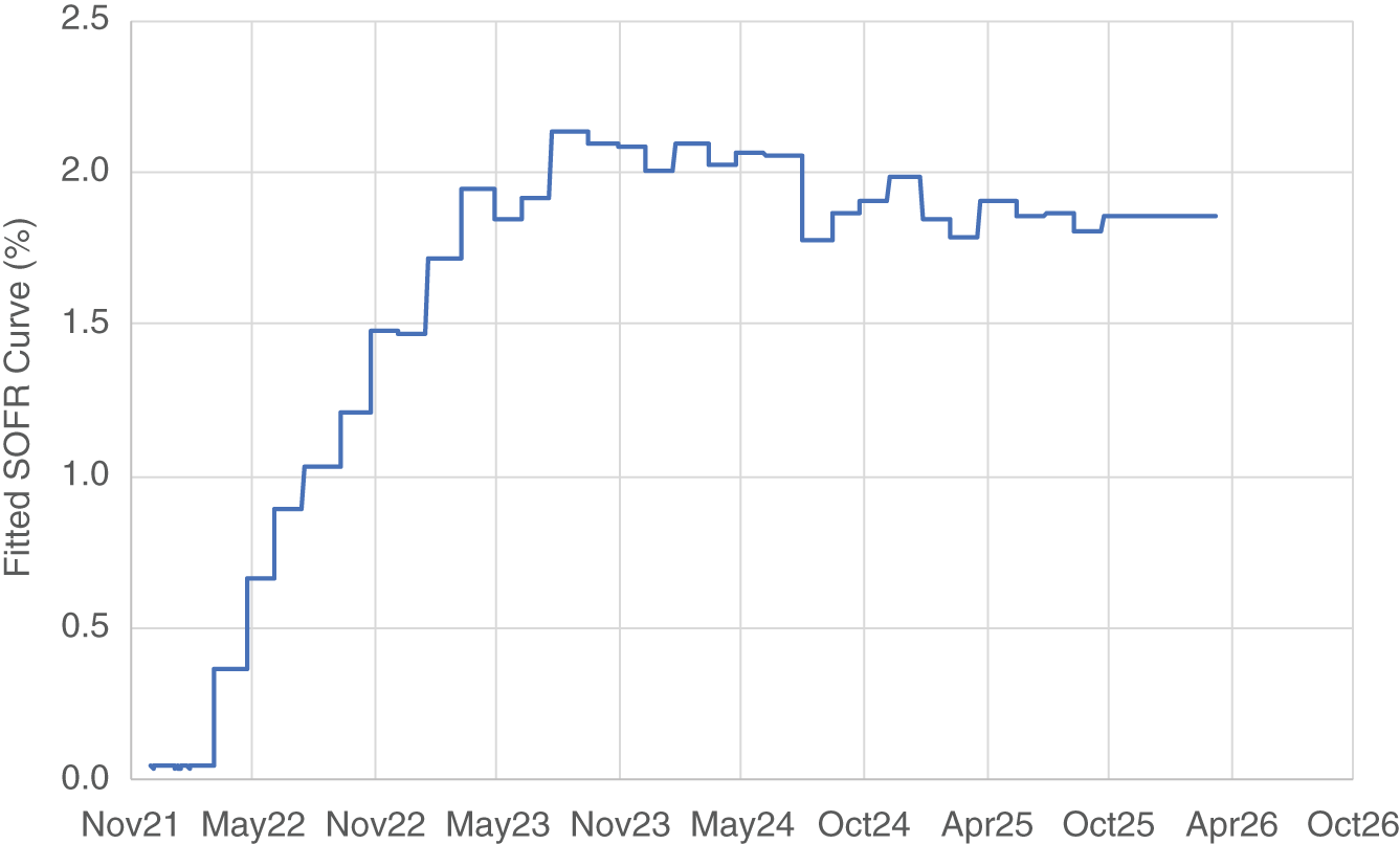
FIGURE 6.4 Fitted SOFR curve
Source: Authors
This curve strikes us as “noisy,” in the sense that the term structure of fitted overnight forward rates appears to oscillate beyond about May 2023 – or at least to experience a series of frequent reversals during this period.
If this series of rate increases followed quickly by rate increases that are soon reversed is genuinely indicative of market pricing, a curve like this might be fine. On the other hand, our a priori belief is that this pattern is more likely indicative of noisy input data than of a series of policy rate reversals.
In an attempt to reduce this noise, we can introduce a regularity condition that increases the smoothness of the step function, where for this purpose we'll define smoothness as the sum of the squared butterfly spreads along the fitted curve.1
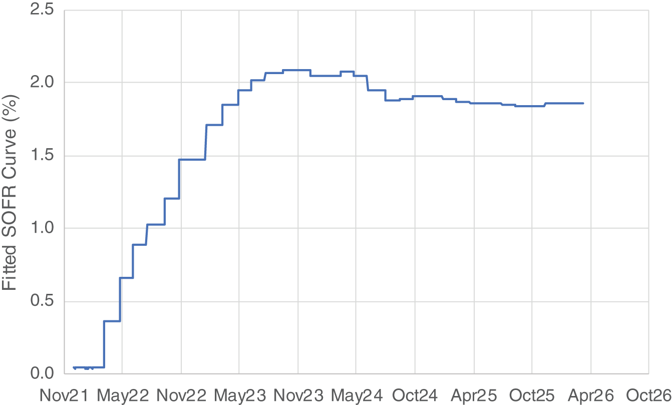
FIGURE 6.5 Fitted SOFR curve with regularity condition
Source: Authors
In particular, we'll choose the heights of the K steps, θ1, θ2, θ3,…, θK, so as to minimize the objective function:
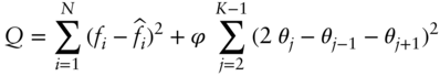
The first summation in this equation is simply the sum of squared differences between the N observed futures prices, fi, and the K fitted futures prices, ![]() . The second summation in the equation is the regularity condition that sums the (K – 2) squared values of the butterfly spreads along the fitted curve. This second summation is scaled by a number, ϕ, that controls the penalty for lack of smoothness.
. The second summation in the equation is the regularity condition that sums the (K – 2) squared values of the butterfly spreads along the fitted curve. This second summation is scaled by a number, ϕ, that controls the penalty for lack of smoothness.
In pushing the curve to be smoother, we necessarily worsen the quality of the fit between the prices of the futures contracts observed in the market and the prices computed along our fitted curve.
The penalty for lack of smoothness can be increased until we obtain a yield curve with an acceptable tradeoff between smoothness and fit. Figure 6.5 provides an example of such a curve.
The tradeoff between smoothness and quality is inevitable, and the choice is necessarily a subjective one for the analyst fitting the curve. But at least the formulation above gives the analyst a framework for assessing the alternatives in this regard.
NOTE
- 1 The butterfly spread between three successive steps is given by (2 × r2) – r1 – r3, where r1, r2, and r3 are the heights of the three steps. The butterfly spread is an approximation to the second derivative of the curve in the segment of the curve containing r1, r2, and r3. The absolute value of a butterfly spread (and hence its square) is relatively large in the presence of a reversal.