
CHAPTER 5
SOFR Future Options
The move from LIBOR to SOFR as reference rate implies a fundamentally new concept: Rather than using a term rate, we apply a daily rate. But SOFR futures combine the daily rates during their reference period into a (forward) term rate. Hence, when dealing with SOFR futures, the situation is similar to LIBOR; in a manner of speaking, one might say that SOFR futures transform the daily rates during their reference period into a term rate like LIBOR. And this is the reason behind the relatively easy transfer of concepts to the new reference rate. Via SOFR futures one does not need to deal directly with daily SOFR, but with the daily SOFR aggregated by the future.
However, once the SOFR futures contract enters its reference period, this aggregation ends and together with it the similarity to LIBOR and the direct transfer of concepts from the Eurodollar (ED) futures market. (Compare Figure 2.1.) As soon as the reference period starts, one needs to deal with daily SOFR values. When only the rate itself is concerned, this can be achieved by some straightforward adjustments for the front-month contract, discussed in Chapter 2 (e.g., for calculating the strip rate and executing the roll). But when volatility is also involved, the end of aggregation at the beginning of the reference period results in a completely new type of option. Before the reference period, options on SOFR futures have a forward term rate as underlying, as do options on ED contracts. But during the reference period, they depend on the path of daily SOFR values during the reference period. Thus, from one day to the next, at the start of the reference period, the same option on the same SOFR future, which used to behave like a standard American option on an ED futures contract, suddenly becomes an Asian option. In the manner of speaking used above, one might say that as SOFR futures enter their reference period, their aggregative function ends – and the options on them therefore transmogrify from standard options on a forward term rate to Asian options.
The fundamentally different concept of the new reference rate, whose practical consequences could be easily managed for futures, therefore manifests itself in a fundamentally different type of options on futures as soon as the reference period starts. From that point onward, one faces the mathematical challenge of pricing Asian options, which is further complicated by allowing jumps in the process. And both the markets using Asian options and the literature dealing with them have so far focused on Asian options of the European type only. Hence, the transfer from LIBOR to SOFR has resulted in a situation in which the options of the key money market (i.e., futures on the reference rate) are options without any pricing model available. From the perspective of options, the migration from LIBOR to SOFR can be considered as an uncontrolled1 experiment: By bureaucratic fiat, the huge market for options on the reference rate is transferred from standard to highly exotic, from being accompanied by well-known pricing models to the absence of any pricing model. And one unintended consequence of the difficulties to price and hedge options on SOFR futures is their lesser suitability for hedging caps and floors – which may explain why market participants seem hesitant to migrate from ED to SOFR futures options.
However, all these challenges are absent before the reference period starts. The aggregation of daily SOFR via the future still works and hence options on SOFR futures are still standard American options with the forward term rate given by the futures as underlying. Since the trading in options on 3M SOFR futures ends before their reference quarter starts, they do not experience the final metamorphosis into exotic options. Hence, they can be priced and analyzed just as options on ED contracts. This allows the transfer of the realized and implied volatility analysis from the unsecured to the secured yield curve – just as Chapter 2 has transferred parts of the yield curve analysis itself. Moreover, the similarity of specifications between options on SOFR and on ED futures enables executing spread positions easily, thereby extending the basis trading from Chapter 4 to options.
Although the decision to let options on SOFR futures expire before they encounter the problem of becoming Asian during the reference period is one possible solution, it comes at the high cost of no options on futures being available until futures settlement. This means that it becomes impossible to hedge a cap or floor with a series of options on SOFR futures in the same manner as one can do with options on ED futures. In other words, the problem of a missing pricing formula for the hedging instrument has been “solved” by the hedging instrument itself being missing. It is similar to healing a wound by amputation.
In contrast to the options on 3M SOFR futures, which end trading before the reference quarter begins, options on 1M SOFR futures end trading together with the underlying contract at the end of the reference month. Hence, these options are subject to the sudden switch to Asian option with American-style exercise. And to make matters worse, they apply the arithmetic average rather than the geometric average, which is even harder to tackle mathematically. On the other hand, while there currently exists no way to price this hedging instrument during the reference month, at least the hedging instrument exists.
In summary, the conceptual difference between a term rate (LIBOR) and an overnight rate (SOFR) is visible within the universe of SOFR futures in the break between the period before and during the reference period and within the universe of SOFR future options in the break between standard and exotic options. It also implies the break between options on 3M and 1M SOFR futures, with only the latter experiencing a sudden transformation during their lifetime. And finally, it implies the structure of this chapter:
- In the first half, we will focus on options on 3M SOFR futures only, exploiting the exclusion of the problem by their specifications. This allows providing an overview over option analysis and trading strategies in general and how they could be applied to SOFR future options – without needing to worry about exotic option pricing. Once more, the concepts can simply be transferred from the unsecured to the secured yield curve and allow new insights into the relationships between the realized and implied volatility along both, which can be exploited easily and cheaply by trading SOFR versus ED futures options spreads.
- In the second half, we will introduce options on 1M SOFR futures and together with them the Pandora's box of pricing American-style Asian options using an arithmetic average. After a brief review of the academic literature on this subject, we will describe the necessary steps toward dealing with these problems, but we will find ourselves without an exact pricing formula. Nevertheless, only by solving this formidable challenge can the full functionality of the key money market can be ensured – by providing options with a similar usability for hedging as the options on ED futures contracts offer. This would also support the liquidity in options on SOFR futures and hence the completion of the transition from the ED complex.
OPTIONS ON 3M SOFR FUTURES: PRODUCT SUITE AND SPECIFICATIONS
Since January 2020, a comprehensive suite of options on the 3M SOFR futures (SR3) has been available. The product suite is summarized in Figure 5.1 and graphically represented in Figure 5.3, while the main technical specifications are listed in Figure 5.2 (Kronstein December 2019).2
SOFR future options are linked to the contract month of the future, i.e., to the beginning of the reference quarter (as defined in Figure 2.2). Correspondingly, trading in options on 3M SOFR futures ends before the reference quarter begins. For instance, the last trading day for the options on the Sep 2022 SR3 future, whose reference quarter begins on Wednesday, 21 Sep, 2022 (included), and ends on Wednesday, 21 Dec, 2022 (excluded), is Friday 16 Sep, 2022. This avoids dealing with the metamorphosis into an exotic option during the reference period. Like for options on ED futures, also options on SOFR futures always refer to a full 3M period of unknown rates, aggregated via the future into one single (forward) term rate.
| Expiries | |
| Standard Options | Quarterly Standard Options for each of the nearest 16 March Quarterly Months (Mar, Jun, Sep, Dec) |
| Serial Standard Options for each of the nearest 4 months not covered by Quarterly Standard Options | |
| 1Y, 2Y, 3Y, 4Y and 5Y Mid-Curve Options | Quarterly Mid-Curve Options for each of the nearest 5 March Quarterly Months (Mar, Jun, Sep, Dec) |
| Serial Mid-Curve Options for each of the nearest 4 months not covered by Quarterly Mid-Curve Options | |
| 3M, 6M, 9M Mid-Curve Options | Quarterly Mid-Curve Options for the nearest March Quarterly Months (Mar, Jun, Sep, Dec) |
| Serial Mid-Curve Options for each of the nearest 2 months not covered by Quarterly Mid-Curve Options | |
| 1Y, 2Y, 3Y Mid-Curve Options | Weekly Mid-Curve Options for each of the nearest 2 Fridays not covered by the options above |
| Strikes | |
| First 4 quarterly and | Intervals of 6.25 bp for a range of 150 bp around ATM |
| first 4 serial options | Intervals of 25 bp for a range of 550 bp around ATM |
| Other options | Intervals of 12.5 bp for a range of 150 bp around ATM |
| Intervals of 25 bp for a range of 550 bp around ATM | |
| (ATM being determined as the strike price closest to the future settlement price of the previous business day) |
FIGURE 5.1 3M SOFR future options: product suite
Source: Authors, based on CME
| Contract size | USD 25 per basis point (USD 2,500 per point per option contract) |
| Style | American |
| Exercise | By notification by 5.30 pm CT of the day of exercise |
| Automatic exercise of ITM options after expiration | |
| Trading venues and hours | CME Globex: 5pm to 4pm, Sun-Fri with a 60-minute break each day beginning at 4pm |
| CME ClearPort: 5pm to 5:45 pm Sun-Fri with no reporting Monday- Thursday from 5:45 p.m.–6:00 p.m. | |
| Open Outcry: 7:20 am to 2pm Mon-Fri | |
| Last trading day | Friday preceding the 3rd Wednesday of the contract month of the underlying future |
| (i.e., the Friday before the beginning of the reference quarter) | |
| Minimum tick size | Quarterly Nearest 0.25 bp if premium not more than 5 bp; 0.5 bp else |
| Second 0.5 bp | |
| Other 0.25 bp if premium not more than 5 bp; 0.5 bp else | |
| Serial 0.5 bp | |
| Block trade minimum size | 625 contracts Asian Trading Hours (4pm–12am, Mon-Fri on regular business days and at all weekend times) |
| 1250 contracts European Trading Hours (12am–7am, Mon-Fri on regular business days) | |
| 2500 contracts Regular Trading Hours (7am–4pm, Mon-Fri on regular business days) | |
| Online resource | https://www.cmegroup.com/markets/interest-rates/stirs/three-month-sofr.contractSpecs.options.html |
FIGURE 5.2 3M SOFR future options: technical specifications
Source: Authors, based on CME
Moreover, as the 3M SOFR future closely mirrors the specifications of the ED future (as discussed in Chapter 2), so the options on the 3M SOFR futures contract have been designed to closely resemble those on ED futures. Together with the margin offset, this facilitates spread trading between both, for example, for exploiting the differences between the volatility of secured and unsecured rates described below. And as part of the transition summarized in Figure Intro.1, options on ED futures “convert” into options on 3M SOFR futures by adding the ISDA spread adjustment to the strike of SOFR options (CME Group 2020).
However, the seemingly similar specifications contain one important difference. When options on ED contracts end trading together with their underlying, they cover the final 3M term rate, while options on SOFR futures end trading before their reference quarters begin. To be more precise, options on SOFR futures end trading on the Friday preceding the third Wednesday of the contract month, while options on ED futures end trading on the Monday preceding the third Wednesday of the contract month – the day on which the SOFR value for Friday is published. As a result, options on SOFR futures end trading not only well before the underlying future ends trading (one business day before the end of the reference quarter), but also before its reference quarter begins, unlike options on ED futures, which end trading at the same time as their underlying contract and thereby cover the full period of the future strip.
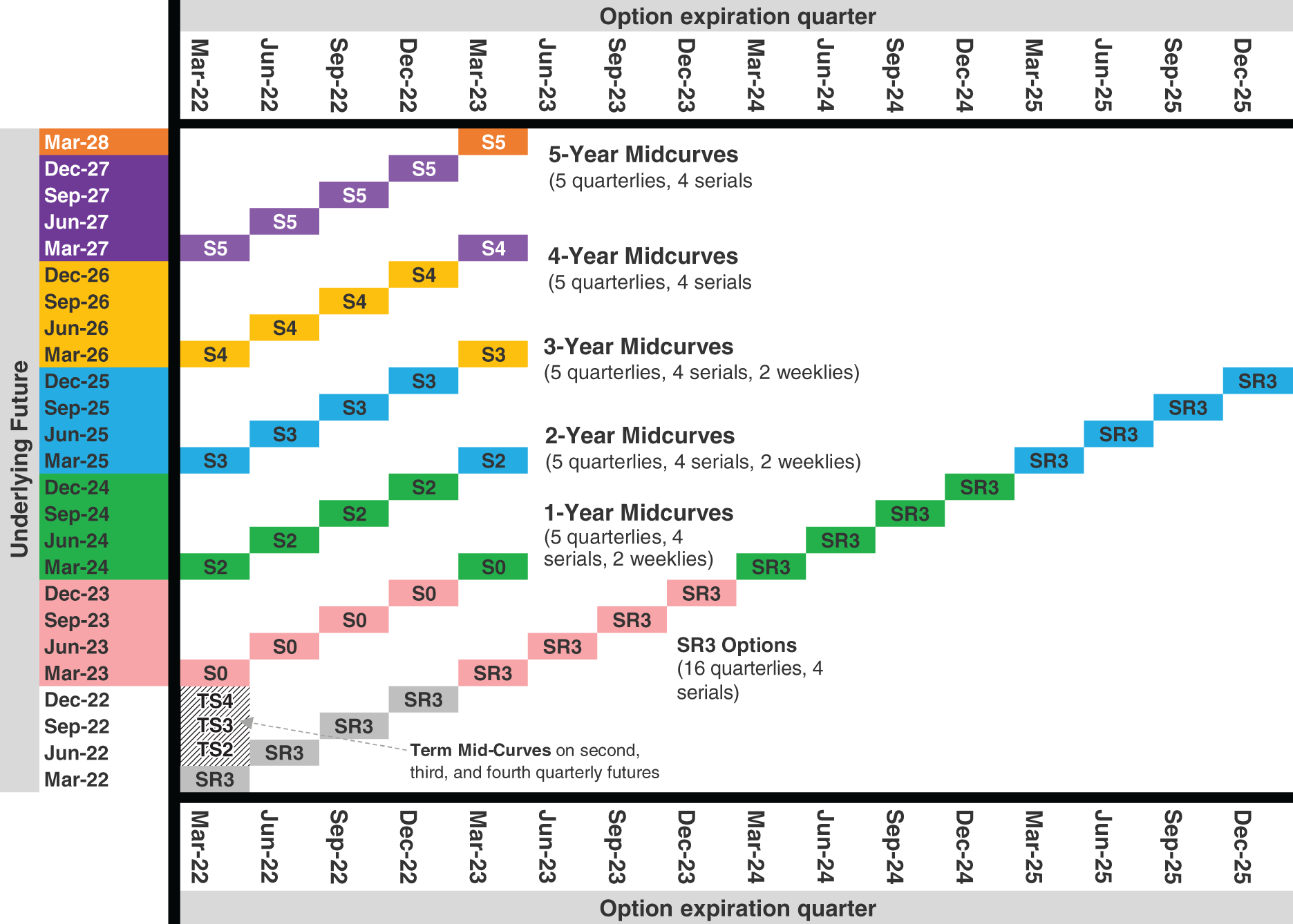
FIGURE 5.3 Options on SR3 futures
Source: CME (Kronstein, Trading SOFR Options, December 2019, Exhibit 1)
This difference has major implications for the usability of future options for hedging caps and floors:
- When options on ED contracts end trading, they refer to the same 3M LIBOR term rate that is used in caps and floors. Hence, a LIBOR-based cap or floor can be easily and (more or less) perfectly hedged with a strip of ED future options, depending on how far the real situation is away from the ideal assumptions.3 Unlike options on SOFR futures, which end trading at about the same time as options on ED contracts, they cover the 3M term rate underlying LIBOR-based caps and floors.
- When options on 3M SOFR contracts end trading, the reference quarter begins, which determines the value of the SOFR-based cap or floor. If volatility were to increase during the reference quarter, it would affect the value of the cap or floor – but there simply exists no option on 3M SOFR futures to hedge against this move anymore. Thus, even an ideal IMM SOFR-based cap or floor cannot be fully hedged with a strip of 3M SOFR future options. In fact, during the reference quarter determining the value of the cap or floor, a hedger could in theory only apply delta-hedging via the front-month contract but would remain exposed to changes in volatility, among other things. And if he uses other options, either other SOFR futures options or OTC derivatives, he incurs spread and model risk and/or high costs.
In general, when the analytic and hedging concepts can be easily transferred from LIBOR to SOFR (futures), SOFR-based products enjoy the easy and cheap hedgeability of LIBOR-products, with the low hedging costs for dealers translating into low transaction costs for end users. When this is not the case, however, the transition from LIBOR to SOFR results in greater hedging costs and thus greater transactions costs. As we have described in Chapter 3 the higher hedging costs of the SOFR term-rate relative to LIBOR, SOFR-based caps and floors are likely to suffer from higher hedging costs than their LIBOR-based counterparts. While in the example of the ideal LIBOR-based cap mentioned above a dealer can make use of the cheap and liquid strip of ED future options for hedging and therefore offer tight bid–ask spreads for the cap, a dealer pricing a SOFR-based cap faces the problem of the 3M SOFR futures option market not offering a hedging instrument during the reference quarter. The dealer therefore either needs to accept unhedged exposure or engage in complex and costly hedging, for example, via OTC derivatives or via using options on 1M SOFR futures as well.4 In both cases, higher hedging costs are likely to result in wider bid–ask spreads.
Moreover, the different ease of hedging SOFR-based swaps with SOFR futures versus the difficulty of hedging SOFR-based caps and floors with SOFR future options may explain why the liquidity in the former has been off to a much better start than in the latter. At the time of writing (Dec 2021), liquidity in options on SOFR futures was still very poor. Hence, while the comprehensive suite of options on ED contracts has been replicated for SOFR contracts (with the important exception of the last 3M), this was still a largely theoretical market, which could hardly be analyzed and traded in practice. During the editing process of this book in the first half of 2022, liquidity has started to pick up. The monthly Rates Recap published by the CME is a good source to obtain information about the current liquidity situation (CME February 2022).5
OVERVIEW OF GENERAL VOLATILITY ANALYSIS
Conceptually, one can classify option analysis and trading in two categories:6
- Implied versus realized volatility. The relationship between the two is achieved via delta hedging and used in the Black-Scholes formula. A consequence is that the current implied volatility quoted in the option market reflects (or, should reflect) the market consensus about the realized volatility of the underlying rate over the life of the option. A view that the realized volatility will be higher than implied can be expressed by buying the option (at the premium determined by the current implied volatility) and delta hedging it. This requires sufficient sensitivity (gamma) of the delta to changes in the yield level and is therefore only practical with options with a short time to expiry (e.g., 3M).
- Implied versus implied volatility. In contrast, options with a long time to expiry (e.g., 5Y) have a low gamma and are thus largely independent from moves in the underlying (hence unsuitable for delta hedging). In other words, options with a long time to expiry can be analyzed and traded almost in isolation from their underlying and its realized volatility. Taken together with their high vega, this makes them suitable for expressing views on the future implied volatility. For example, the expectation that implied volatility will increase over the next few months can be expressed by buying a straddle with 5Y expiry and unwinding it after a few months. The lower sensitivity of long expiry options to their underlying instruments also makes them suitable for analyzing and trading the relationships between implied volatility, for example, via a principal components analysis (PCA) on the volatility surface or cube (Huggins and Schaller 2013, p. 336).
In summary, options with short expiries are suitable for expressing views about the future realized volatility (relative to their price, i.e., their current implied volatility) via delta hedging; options with long expiries are suitable for expressing views about the future implied volatility (relative to their price, i.e., their current implied volatility). Correspondingly, spreads between options with short expiry are suitable for expressing views about the future realized volatility curve (i.e., for RV trades of the future realized volatility curve versus the current implied volatility curve); spreads between options with long expiry are suitable for expressing views about the future implied volatility curve (i.e., for RV trades of the future implied volatility curve versus the current implied volatility curve) (Huggins and Schaller 2013, p. 346).
When applying these general concepts to options on SOFR futures, we face the problem of low liquidity. Specifically, the first step for analyzing implied volatility is the creation of constant time-to-expiry and constant delta time series, for example, by calibrating an (SABR-)model to the volatility cube. One can then analyze the historical behavior and relationships between the implied volatility of different parts of the volatility cube and consider mismatches, e.g., PCA residuals, as candidates for trading opportunities. While options on futures are in principle a good area for this analysis due to their usually low transaction costs, the preconditions for this analysis are still lacking, since in the absence of a liquid market it could only observe its own assumptions rather than actual prices.
Given this situation, we focus first on analyzing the realized volatility of SOFR futures, which is independent of both the missing pricing model and the missing liquidity of options, and we describe the distribution of realized volatility over the secured yield curve and its evolution over time. We will then mention the connection of this analysis of realized volatility with implied volatility and describe possible trades. Since there exist some attractive trading strategies with options on SOFR futures, in particular spread positions versus options on ED contracts, this could support the migration to a liquid SOFR future options market.
DISTRIBUTION OF REALIZED VOLATILITY OVER THE SECURED YIELD CURVE
For analysts, the introduction of SOFR futures is a milestone in general, as they provide market prices for secured rates for consecutive 3M forward periods. This allows repeating the analytic methods developed for the unsecured curve (e.g., the ED future strip) for the secured curve and to add an analysis of the spread, i.e., the unsecured–secured basis. Applying this general idea to options, we will first repeat the analysis of realized volatility for the secured yield curve as given by 3M SOFR contracts and then extend it considering the spreads between realized volatility on the secured and unsecured yield curves.
The time series of SOFR futures has allowed us in Chapter 2 to extract a history of consecutive 3M forward rates for the secured yield curve and allows us now to calculate a history of the realized volatility curve for secured rates. While this has been possible for unsecured rates via ED futures for many years, the concentration of liquidity in the repo market on overnight market has until now prevented the transfer of this analysis to the market for secured lending.
Using the SOFR future data shown in Figure 2.5, we have calculated the evolution of the realized volatility curve (normal volatility, annualized) for secured rates over time and exhibit the results in Table 5.1. In more detail, we have divided the dates into approximate reference quarters, spanning from the 20th of March to the 20th of June, etc. The beginning of these 3M periods is indicated by “Jun-18” etc. in Table 5.1. We have then calculated the realized volatility for each of the SOFR futures during these 3M periods and thereby obtained the realized volatility curve for consecutive 3M forward periods. “3M,” “6M,” etc. in Table 5.1 refer to the approximate forward dates. For example, the first entry of 12 bp for “Jun-18/3M” refers to the realized volatility of the Sep 2018 SOFR future during the time period from 20 June 2018 to 19 Sep 2018, i.e., roughly during the period of the reference quarter of the previous contract.
TABLE 5.1 Realized volatility in different parts of the secured rate curve over time (normal in bp, annualized)
Source: Authors, based on data from CME
| 3M | 6M | 9M | 12M | 15M | 18M | 21M | 24M | |
|---|---|---|---|---|---|---|---|---|
| Jun-18 | 12 | 19 | 24 | 29 | 32 | 32 | 33 | #N/A |
| Sep-18 | 13 | 22 | 28 | 35 | 39 | 42 | 44 | 45 |
| Dec-18 | 23 | 36 | 45 | 54 | 60 | 64 | 67 | 67 |
| Mar-19 | 24 | 53 | 68 | 77 | 83 | 85 | 85 | 83 |
| Jun-19 | 68 | 85 | 91 | 99 | 102 | 104 | 104 | 104 |
| Sep-19 | 38 | 55 | 64 | 73 | 78 | 81 | 84 | 85 |
| Dec-19 | 92 | 84 | 79 | 76 | 76 | 78 | 81 | 83 |
| Mar-20 | 13 | 17 | 19 | 22 | 26 | 29 | 35 | 39 |
| Jun-20 | 6 | 8 | 8 | 10 | 11 | 13 | 16 | 16 |
| Sep-20 | 5 | 6 | 7 | 9 | 10 | 11 | 13 | 15 |
| Dec-20 | 7 | 8 | 8 | 7 | 9 | 12 | 19 | 28 |
| Mar-21 | 7 | 6 | 6 | 8 | 15 | 21 | 29 | 39 |
| Jun-21 | 6 | 6 | 9 | 16 | 23 | 33 | 44 | 53 |
Figures 5.4 and 5.5 slice through the two dimensions of Table 5.1. This corresponds to the slicing of Figures 2.6 and 2.7 for the level of consecutive 3M forward rates. Figure 5.4 depicts the evolution of the realized volatility in different consecutive 3M forward periods over time. Overall, realized volatility has increased as the Fed started to cut rates, but it reached its peak well before the Fed was done cutting. Unsurprisingly, realized volatility has been low across the curve as long as interest rates were expected to be anchored close to zero for an extended period of time. More recently, uncertainty about the future path of Fed policy has affected volatility in the longer part of the curve more than at the short end. The specific behavior of the shortest part of the curve, which has reached the peak well after the other parts, is remarkable.
Figure 5.5 shows the realized volatility curve at different points in time. With the exception of the period covering 20 Dec 2019 to 19 Mar 2020 (corresponding to the peak of realized volatility for the shortest part just mentioned), realized volatility curves have been upward sloping, reflecting uncertainty about Fed policy increasing with the forwards.
Chapters 2 and 5 have illustrated how SOFR futures allow transferring established analytic concepts from the unsecured to the secured yield curve and its volatility. Combining both,7 one can replicate the analysis from Burghardt (2011) and Ilmanen (1995) and calculate the historical average Sharpe ratios for investing in different consecutive 3M forward periods of the secured yield curve. Figure 5.6 shows the results of this exercise, i.e., the Sharpe ratio of holding a SOFR future corresponding to a specific consecutive 3M forward part (“3M,” “6M,” etc. in Table 5.1), taking the average over the 3M holding periods (“Jun-18,” “Sep-18” etc. in Table 5.1). It appears that the Sharpe ratio is highest around the 9M forward point on the secured yield curve, which remarkably is quite in line with the results from Burghardt and Ilmanen from years earlier.
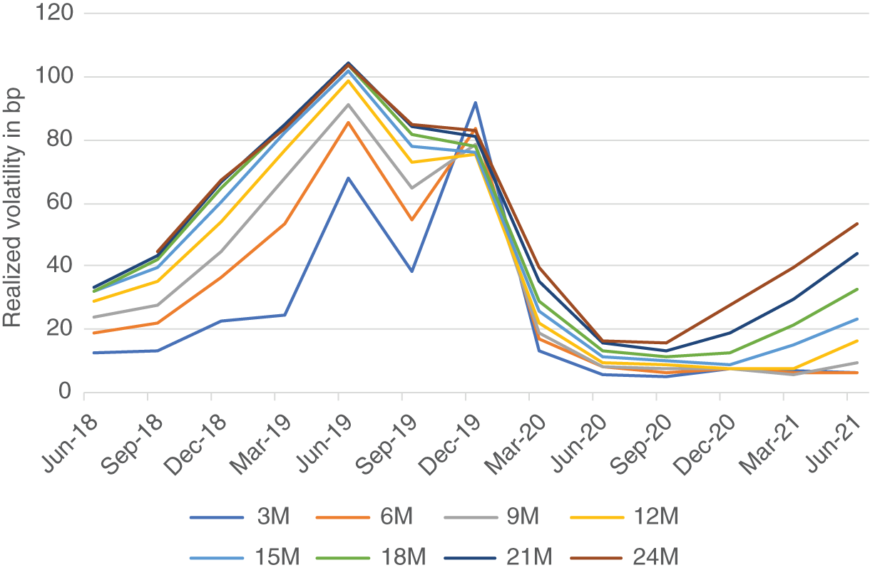
FIGURE 5.4 Realized volatility (normal in bp, annualized) of the secured rate curve
Source: Authors, from CME data
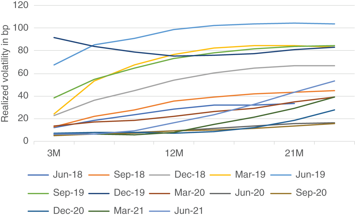
FIGURE 5.5 Realized volatility (normal in bp, annualized) of the secured rate curve
Source: Authors, from CME data
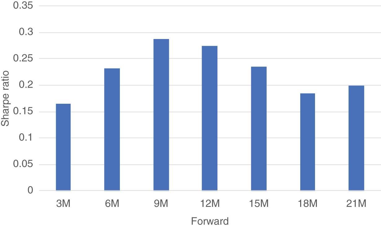
FIGURE 5.6 Average Sharpe ratios for the SOFR future curve
Source: Authors, from CME data
Given the short time period of available data, the results of these analyses should be considered to be preliminary, and they need to be repeated when a longer history – post SRF introduction – will have become available.
CURRENT IMPLIED VERSUS HISTORICAL REALIZED VOLATILITY
While an illiquid market prevents historical implied volatility analysis (e.g., via a PCA on the volatility cube), it is still possible to compare current implied volatility quotes, whenever they are observable, with the historical realized volatility. Graphically, this can be done by adding the current implied volatility curves in the chart (Figure 5.5) depicting the historical evolution of realized volatility curves. Figure 5.7 shows an example with the implied levels for ATM forward quarterly standard options observed on Dec 10 and 17, 2021.
This comparison allows assessing which historical realized volatility scenario is implied by the current market, both with regards to the overall level of volatility and to the shape of the volatility curve (Huggins and Schaller 2013, p. 327). If it turns out that the current implied volatility curve is extreme or abnormal relative to the range of historical realized volatility curves, it may be a candidate for an implied versus realized volatility (curve) trade via delta hedging, as described above. Also, analysts can use Figure 5.7 to assess which Fed policy scenario is currently implied in the SOFR future options market and, in case their view differs from the implied scenario, use these instruments to express their view via an option (curve) trade.
Again, the limited length of SOFR history still limits the strength of this analysis. In general, it is subject to the structural break due to the introduction of the SRF described in Chapter 1. In particular, the data of Figure 5.7 contain no realized volatility curve calculated during a period of sustained Fed rate hikes. In order to illustrate how this analysis could be performed once enough (post-SFR) data will have become available, let us counterfactually assume that the range of historical realized volatility curve scenarios shown in Figure 5.7 was complete. One could then conclude that the implied volatility curve as of December 10, 2021, was both on a high level and steep relative to the range of historically observed realized volatility curves. If an analyst does not see a good reason for this (and speculation about Fed hikes could be such a good reason not reflected in the data yet), there are two possible trades:
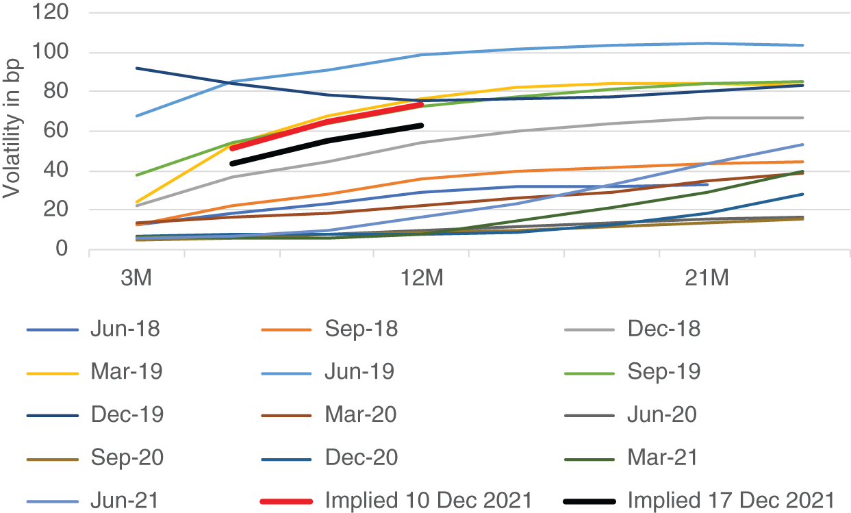
FIGURE 5.7 “Current” implied versus historical realized volatility along the secured rate curve
Source: Authors, from CME data
- A position on the level of implied versus realized volatility. This involves selling options on SOFR futures and delta hedging them, thereby obtaining the difference between the (high) current implied volatility and (expected lower) realized volatility as profit. In this case, the shape of the current implied volatility curve can be used for selecting the best (i.e., most overvalued) option for this trade. While the shape of the volatility curve is not directly traded, it influences the asset selection.
- A position on the slope of the implied versus realized volatility curve. This involves selling 12M and buying 6M options on SOFR futures and delta hedging both of them, thereby obtaining the difference between the (high) steepness of the current implied volatility curve and the (expected flatter) realized volatility curve as P&L. This possibility directly trades the shape of the volatility curve.
Usually, the second alternative involves higher transaction costs, some of which can be mitigated by margin offsets, but also lower risk due to a (perhaps imperfect8) hedge of the exposure to the overall level of volatility. Which one of the two possibilities is best in a given situation can be assessed by calculating their Sharpe ratios (after transaction and delta hedging costs) in several different scenarios. When selecting the second alternative, the different expiries of the options also need to be considered, as delta hedging until (close to) the expiry of the shorter option is typically not practicable.
Figure 5.7 also contains the implied volatility curve for Dec 17, 2021, after a Fed meeting which clarified the future policy to a certain extent. As one would expect, the lower uncertainty has resulted in a lower overall level of implied volatility, while the implied volatility curve has remained steep. Under the counterfactual assumptions and caveats from above, on Dec 10, 2021, the first alternative might have been better (and performed well during the first week), while on Dec 17, 2021, the second alternative might have offered the more attractive risk/return balance.
OPTIONS ON SOFR FUTURES VERSUS OPTIONS ON ED FUTURES
In the general discussion of the analytic implications of the introduction of a secured yield curve via SOFR futures to the universe of possible trades, we have claimed that, in addition to replicating the analysis for the unsecured yield curve (Chapter 2) and realized volatility curve (Chapter 5) for the secured yield curve, new analytic concepts between both have also become possible. Chapter 4 has provided the first steps for this new analysis of the secured–unsecured basis for the yield curve. This chapter extends it to the realized volatility curve.
The equation from Chapter 4 linking unsecured (LIBOR) and secured (repo) rates allowed the conclusion that the LIBOR–repo spread tends to increase when rates increase. This translates directly to an argument for higher (realized) volatility of LIBOR than of repo rates: When rates increase, LIBOR tends to increase more than repo; when rates decrease, LIBOR tends to decrease more than repo. Hence, LIBOR tends to move more than repo.
This argument has been used to explain the observation of (LIBOR-based) swaption volatility usually exceeding bond option volatility (Huggins and Schaller 2013, p. 325). Likewise, it can be used to explain the observation of ED future volatility usually exceeding SOFR future volatility visible in Figure 5.8.9 However, as explained in Chapter 4, while the rate level remains an important factor driving the secured–unsecured basis (Table 4.2), it is not the only driving factor. Hence, whereas the argument is still valid, at times it may be overpowered by other influences. For example, the spikes in SOFR during 2019 may explain the “abnormal” period of realized SOFR future volatility exceeding realized ED future volatility.
Chapter 4 assessed the likely effects of the additional driving forces mentioned in Chapter 1 on the unsecured–secured basis. Translating the results in terms of realized volatility, an increase in the costs of executing the arbitrage between secured and unsecured lending rates gives more room for SOFR to move. According to this analysis, when these costs increase, SOFR has more room to increase before hitting the arbitrage boundary. Hence, in times of high costs, for example, when the marginal bank faces balance sheet constraints, it is possible that the volatility in SOFR increases relative to the volatility of EFFR.10 This may explain the atypical period of realized SOFR futures volatility exceeding realized ED futures volatility.
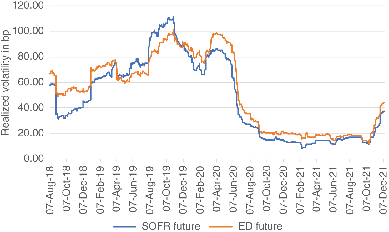
FIGURE 5.8 Realized volatility (normal in bp, annualized) of the Jun 2022 ED and SR3 futures
Source: Authors, from CME data
By contrast, the reaction of the Fed to these SOFR spikes of introducing the SRF has imposed an upper bound on SOFR but not on EFFR. In terms of realized volatility, the effect of this measure is therefore a reduction in realized SOFR volatility, both on an absolute level and relative to unsecured rates, which are not (directly) affected by the upper bound. In a certain sense, greater regulatory costs have relaxed the boundary for SOFR and the SRF has established a new boundary for SOFR. This may explain why, after the introduction of SRF, no atypical periods of realized SOFR future volatility exceeding realized ED future volatility have been observed.
Taken together, one might conclude that, while the argument for higher realized volatility of unsecured than secured rates based on the formula from Chapter 4 needs to be expanded with additional considerations, it is still largely valid.
Given the realized volatility relationship, a situation in which the implied volatility of options on SOFR futures exceeds the implied volatility of options on ED futures11 can be considered as a potential trading opportunity, in particular if the Fed reaction to the SOFR spikes during 2019 is deemed sufficient to prevent repetitions.
In fact, analysts may want to monitor the STIR market for these additional opportunities provided by volatility spreads between secured and unsecured rates. Due to the significant margin offset between options on ED and SR3 contracts, future markets provide a much cheaper way to trade the general argument of the realized volatility of unsecured rates usually exceeding the realized volatility of secured rates than by trading swaptions versus bond options. And the suitability of options on SOFR futures for these RV trades versus options on ED futures may support the migration of liquidity toward the former.
OPTIONS ON 1M SOFR FUTURES: PRODUCT SUITE AND SPECIFICATIONS
Since May 2020, options on the 1M SOFR futures (SR1) contract also have been listed (CME April 2020). The product suite is summarized in Figure 5.9, while the main technical specifications are listed in Figure 5.10.
The key difference to the specifications of options on 3M SOFR futures is that both the 1M SOFR futures contract and the options on it end trading on the same day, i.e., on the last business day of the contract month. This difference in specifications has two major consequences:
- Unlike options on 3M SOFR futures, options on 1M SOFR futures undergo the transmogrification into an exotic Asian option during their lives.
- Unlike options on 3M SOFR futures, options on 1M SOFR futures provide a complete series of hedging instruments for caps and floors.
| Expiries | Monthly Standard Options for each of the nearest 4 months |
| Strikes | Intervals of 6.25 bp for a range of 62.5 bp around ATM |
| Intervals of 12.5 bp for a range of 125 bp around ATM | |
| (ATM being determined as the strike price closest to the future settlement price of the previuous business day) |
FIGURE 5.9 1M SOFR future options: product suite
Source: Authors, based on CME
| Contract size | USD 41.67 per basis point (USD 4,147 per point per option contract) | |
| Style | American | |
| Exercise | By notification by 5.30 pm CT of the day of exerise | |
| Automatic exercise of ITM options after expiration | ||
| Trading venues and hours | CME Globex: 5pm to 4pm, Sun-Fri | |
| CME ClearPort: 5pm to 4 pm Sun-Fri | ||
| Last trading day | Last business day of the contract month | |
| (i.e., on the same day as the underlying 1M SOFR future) | ||
| Minimum tick size | 0.25 bp (USD 10.4175) | |
| Block trade minimum size | 250 contracts | Asian Trading Hours (4pm–12am, Mon–Fri on |
| regular business days and at all weekend times) | ||
| 500 contracts | European Trading Hours (12am–7am, Mon–Fri | |
| on regular business days) | ||
| 1000 contracts | Regular Trading Hours (7am–4pm, Mon–Fri | |
| on regular business days) | ||
FIGURE 5.10 1M SOFR future options: technical specifications
Source: Authors, based on CME
Thus, by virtue of the specifications of options on 1M contracts, at least there is a complete strip available for hedging purposes. But the tradeoff is that there is no pricing model. Extending the strip until the end of the life of the future closes the gap versus caps and floors – by extending the life of the options into the period when they become exotic.
When considering options on 1M SOFR contracts, the problem of dealing with Asian options cannot be avoided any longer, as it could be avoided by exploiting its exclusion by the specifications of options on 3M SOFR futures. And the choice of arithmetic averaging and American-exercise type in the specifications for options on 1M SOFR futures results in one of the most difficult pricing problems, which will be described below.
The other way around, the characteristics of Asian options can explain some of the behavior observed during the reference period of SOFR futures, specifically the decreasing volatility of the underlying future contract during its reference period due to the increasing number of SOFR values becoming fixed. (See Figure 2.5 and Chapter 9.) In fact, while options ending at the beginning of the reference period face the issue of unstable Greeks immediately before expiry, this problem is mitigated by the decreasing sensitivity of the underlying futures contract during its reference period. Intuitively speaking, while the gamma of an at-the-money (ATM) option goes toward infinity as the option approaches expiry, independent of whether the expiry is set at the beginning or at the end of the reference quarter, at the end of the reference quarter the volatility of the underlying SOFR future goes to zero, which might solve the problem. In the absence of a pricing model there is currently no way to quantitively express and to prove the intuition behind this argument (unless one relies on boundary conditions).
In Chapter 10, we will cover the second of these two major consequences in more detail and discuss hedging caps and floors with a combination of options on 3M and 1M SOFR futures. For the moment, we note that while it is possible in principle to hedge a cap or floor with calendar monthly resetting dates with a strip of options on 1M SOFR futures, the limited product suite limits the reach of this hedging method in two dimensions:
- As options on 1M SOFR futures are limited to the next four months (compare Figures 5.1 and 5.10), only very short caps or floors can be hedged with them alone. For longer caps and floors, a combination of options on 3M and 1M contracts must be used. But since the dates do not match, there will be either an overlap or a gap between the strip of options on 3M and the strip of options on 1M futures. And in the absence of a pricing model, it will be hard to assess and hedge the overlap or gap – leading to higher bid–ask spreads again.
- The strike prices of options on 1M SOFR futures do not cover a very large range. Thus, for hedging far out-of-the-money caps and floors, only the strikes of options on 3M SOFR futures can match the strikes – but not the period of the cap or floor to be replicated or hedged.
While the need to deal with Asian options is necessary if we want a complete series of hedging instruments, leading to an unavoidable mathematical complication of the transition from LIBOR to SOFR, some of the specifications seem to make the migration unnecessarily difficult:
- The product suite of options on 1M SOFR futures could be expanded to cover a wider range of periods and strikes.
- Applying daily compounding (rather than using an arithmetic average) also for 1M SOFR futures, which we recommended in Chapters 2 and 3 for different reasons, would also result in much easier pricing of the options, as discussed below. The ensuing difference to the specifications of FF futures could be solved by applying daily compounding to all STIR futures contracts.
- If options on 3M SOFR futures ended trading together with their underlying contract (as do options on 1M SOFR futures), there would at least exist a complete strip of hedging instruments for caps and floors. And since these involve daily compounding, the pricing problem seems to be somewhat easier to solve.
- This could also be an opportunity to consider European-style exercise rather than American-style exercise for options on both the 1M and 3M SOFR futures. For Asian options of the European type using geometric averaging, a pricing formula already exists. An additional advantage is the alignment of the hedging instrument with caps and floors, which usually are of the European type. And again, the ensuing difference to the specifications of FF and ED futures could be solved by switching all STIR contracts to the European-exercise type.
At the time of writing, liquidity in options on SOFR futures is still held back by both the absence of a pricing model and the absence of a complete product range for hedging caps and floors. In turn, the low liquidity of options on SOFR contracts seems to hold back the full migration from ED futures, since capped or floored loans can still be more effectively hedged with options on ED contracts. In order to complete the transition and to enjoy a functioning option market for the key money market rate after the switch to SOFR, a concerted effort of academics, market participants, and the CME seems necessary, with the specifications taking into account the current status and further evolution of pricing models.
OVERVIEW OF AVAILABLE PRICING MODELS FOR ASIAN OPTIONS
All pricing models for Asian options in the literature known to us treat the European exercise type only (Horvath and Medvegyev 2016 contains a relatively easy introduction). Applying them to the American type of CME's options on SOFR futures is therefore a general and presumably difficult problem.
Assuming continuous geometric Brownian motion and a geometric average as determinant of the payoff of the option, the Black-Scholes approach can be replicated to price Asian options fulfilling these conditions. From this starting point, Asian options that do not satisfy these conditions have been tackled in various ways:
- When an arithmetic average is used as determinant of the payoff of the option (which is more common in the market than a geometric average), there does not seem to exist a pricing formula. Instead, Monte Carlo simulations (applying the geometric average as control variate) (Kemna and Vorst 1990), Laplace transformations (Geman and Yor 1993), and approximations/boundaries (Vyncke, Goovaerts, and Dhaene 2003) have been studied.
- The second relaxation of the assumptions required for application in actual markets is the replacement of continuous with discrete processes. Vyncke, Goovaerts, and Dhaene (2003) present an analytic approximation for an arithmetic average over a discrete process. As the first and second moments match, the approximation allows calculating the Greeks. We have implemented and tested this model in the iron ore complex.
- Finally, and of key importance for money markets dealing with jumps, a wider variety of processes is allowed. Fusai and Meucci (2008) tackle Asian options on discretely monitored Lévy processes, which include mixed jump-diffusion models, and obtain (via Fourier transformations) a pricing formula for geometric averages and (via recursive integration) a formula for the moments for arithmetic averages.
Checking the available models for their suitability to price options on SOFR futures, we find:
- The general problem of American versus European type: Since all literature known to us assumes European type, either the literature needs to be transferred to the American type (which does not seem trivial), or CME needs to change the specifications to European (which seems to be the easier of the two possibilities).
- Options on 1M SOFR futures, which use an arithmetic average, are subject to the generally harder accessibility compared to the geometric average. The usual approach of the papers mentioned above is to transfer the results from the geometric to the arithmetic case, thereby needing to replace pricing formulas with approximations or simulations.
- Options on 3M SOFR futures use compounding according to the ISDA formula from Chapter 2. Unfortunately, the method of multiplying the SOFR value with the number of the days for which it is used (e.g., with three, in case of a weekend) results in the settlement rate of 3M SOFR futures being theoretically different from a strict geometric average. Particularly at the current low interest rate level, however, it seems likely that this difference is negligible from a practical point of view. There is thus reason for optimism that options on 3M SOFR futures can be treated as settling to a geometric average, which is relatively easy to access, and for which pricing formulas exist in case of European-exercise Asian options.
- Taking into account the importance of jumps (due to Fed policy changes) in the money market, models only allowing for (geometric) Brownian motion seem rather unsuitable for our task. In Chapter 2, we surveyed a few possible processes for pricing futures, with a mixed jump-diffusion process (with drift) being the most general form. Fortunately, these processes are all covered by the Lévy process treated in Fusai and Meucci (2008).
A POSSIBLE ROAD MAP TOWARD PRICING OPTIONS ON SOFR FUTURES DURING THE REFERENCE PERIOD
Given the situation the practical dealer in options on money market futures has been put in by the migration from LIBOR to SOFR and the imperfect theoretical remedies available, the following describes steps for one possible way forward:
- The choice of model is fundamental. As discussed at the end of Chapter 2, a mixed jump-diffusion process (potentially with drift) seems to be both conceptually reasonable (covering jumps from Fed policy changes and also unrelated volatility) and practicable. This process could be used to price both SOFR futures and their options, thereby avoiding mismatches from using different models for both. By contrast, this process is different from the simple jump-only step function used for CME's term rate. As discussed in Chapter 3, this is likely to result in mismatches between futures and options on one hand (priced via a jump-diffusion model) and the term rate (priced via a step function). However, as a pure step function is unsuitable to price options, this mismatch is unavoidable – as long as the CME sticks to its term rate calculation. If a trader is only concerned with pricing SOFR futures, he can consider using the same approach that CME applies for the term rate; once he also deals in options, he will encounter mismatches due to different models and can only choose where the discrepancy occurs – between futures and the term rate on one hand (both using jump-only) and options on the other hand, or between futures and options on one side (both using mixed jump-diffusion) and the term rate on the other side.
Moreover, it needs to be determined whether the model should incorporate the spread between secured and unsecured rates by being calibrated to all STIR contracts at once. (See Chapters 2 and 4.) While this is advisable when focusing on the effect of the secured–unsecured basis on the relative pricing in the STIR universe, as we did in the last chapter, when applied to options, it would incorporate the spread between standard options on unsecured rates (ED and FF contracts) and exotic options on secured rates (SOFR contracts), i.e., add another layer of complexity to an already difficult task. Hence, for dealing with options, separate models for unsecured and secured rates seem to be more practicable. Here, the model tradeoff therefore is between the applicability for analyzing the secured–unsecured basis and the practicability for option pricing.
Finally, as mentioned in Chapter 2, a key consideration is the link between the jumps and the mean reversion (drift) in the model. For example, one needs to decide whether a rate hike should be treated as part of the mean reversion or not (and hence the mean being shifted to the same extent).
- Based on the model selection, the appropriate option pricing model needs to be developed by building on the available literature. For our preferred process choice of a mixed jump-diffusion model, Fusai and Meucci (2008) seems to be a useful starting point, offering a pricing formula for geometric averages. Assuming 3M SOFR futures to be close enough to this assumption,12 the only remaining major problem to be solved appears to be the adjustment from European- to American-style exercise. In the absence of a closed-form solution, numerical methods can be used to obtain an approximation.
- Finally, the pricing needs to work in practice. This step requires data aggregation and encoding. In case of numerical methods such as Monte Carlo simulations being involved, the challenges and running time should not be underestimated (Horvath and Medvegyev 2016). Before being applied to actual trading, extensive testing is advisable. While at the time of writing, the illiquidity of the SOFR future options market prevents any testing, it is possible that by the time of publication, candidates for pricing models can be assessed against an actual market – and vice versa enhance its liquidity by improving the usability of options on SOFR futures as hedging product.
Of these three steps, we will focus on the first one and assess in the next section the effect of model selection on the option prices – using our heuristic sheet from Chapter 2 in the absence of a pricing model.
IMPACT OF PROCESS SELECTION ON THE PRICING OF OPTIONS ON SOFR FUTURES
The first step of selecting a process is independent of the second step of selecting a pricing framework – and also independent of transition from standard to exotic options. In fact, the issue of choosing an appropriate process for modeling money market options is well known from pricing options on ED futures.13 Under the realistic assumption of the Fed policy having a major effect on short-term rates, it makes sense to include jumps at the FOMC meeting dates (and maybe also around the quarter end) in the process. As described in Chapter 2, one may decide to use a combined jump-diffusion process or a spline with the FOMC meetings as external variables. The disadvantage of including jumps is that option-pricing models based on assuming continuous Brownian motion become unapplicable. Thus, one needs to build an option-pricing model accounting for the jumps. If one assumes that the rate is constant between the FOMC meetings (which is also unrealistic since it ignores all other sources of rate volatility), one can try and construct a tree. One problem with this approach is the unknown jump sizes, which could be addressed by allowing only 25 bp jumps, for example, resulting in a further move away from reality. And since high volatility often coincides with unscheduled FOMC meetings, this approach does not capture some of the biggest events for short rate volatility.
Similar to the way we used a similar spreadsheet in Chapter 2 to assess the influence of model and parameter selection on the pricing of SOFR futures, we can now expand this sheet to demonstrate the effects of different processes on the prices of options on SOFR futures. Again, we have simulated the evolution of SOFR via a Vasicek process with and without jumps. Of course, this approach can be subjected to the criticism we have just summarized in addition to the criticism from Chapter 2, specifically the absence of a consideration of the link between the drift term of the Vasicek process and the jumps. Therefore, it should be considered as an initial heuristic attempt only.
The simulation is encoded in the Excel worksheet “Call simulation” accompanying this chapter, which is a slight modification and expansion of the sheet “SOFR future price simulation” from Chapter 2. We assume that on Jan 1, 2022, one wants to price a call on the Mar 2022 SR3 contract. During its reference quarter (from Mar 16 to Jun 15), there is one scheduled FOMC meeting, on May 4, 2022. Unlike in Chapter 2, we assume that there is zero probability for a change in Fed policy outside of this meeting, including on the two FOMC meetings before the start of the reference quarter.
Like in Chapter 2, column E defines the parameters for the Vasicek process and the probability distribution for the jump at the FOMC meeting(s). Based on this input, starting in row 15, the SOFR evolution is simulated, assuming the standard deviation to be the same for each calendar day. Again, we use only 200 simulations (in the columns), which is significantly too little. When used in a trading context, many more simulations, such as 1,000,000, are required. For each of the simulated paths, the payoff of a call (with the strike level being set in cell H1) is calculated – under the assumptions of a European-type option exercisable at the end of the reference quarter, i.e., the two changes to the specifications we have recommended above. The average payoff over all simulations is displayed in cell H4. Of course, this is not the option price as obtained via an option pricing model. The goal of the exercise is not to present a pricing model, but a heuristic framework to give a sense for the issues involved in process and parameter selection. In terms of the steps mentioned above, we try to get some sense for the process (step 1) to be used for building a pricing model (step 2).
Table 5.2 exhibits the results for a few different combinations of parameters for the jump-diffusion (and drift) process. For this table, we have only changed two parameters, the standard deviation of the diffusion process and the probability of the +25 bp jump at the May 4 FOMC meeting,14 which allows displaying the results in the form of a matrix. The other parameters were kept stably at a SOFR start value on Jan 1, 2022, of 0.05%, a mean of 1.5%, a speed of mean reversion of 0.002, and a strike of 100.
TABLE 5.2 Simulated average payoff of a call on the Mar 2022 SR3 future with a strike at 100 (annualized, bp)
Source: Authors
| Standard deviation (ann) | |||||
|---|---|---|---|---|---|
| 0% | 1% | 2% | 5% | ||
| Probability of a 25 bp hike | 0% | 0.0 | 1.9 | 6.3 | 20.2 |
| 20% | 0.0 | 1.8 | 6.1 | 19.2 | |
| 40% | 0.0 | 1.5 | 6.0 | 18.3 | |
| 60% | 0.0 | 1.3 | 4.8 | 17.6 | |
| 80% | 0.0 | 1.1 | 4.5 | 17.0 | |
| 100% | 0.0 | 1.0 | 4.3 | 16.6 | |
In line with the goal of this demonstration, we observe a high dependency of the results on the process and parameter selection:
- A pure jump process – under the assumption of no probability for a rate cut (and ignoring other considerations like margins) – results in an average payoff of 0.
- A pure diffusion and a combined jump-diffusion (with drift) process both assign a considerable value to a call with strike 100, with the value depending highly on the volatility parameter used for the Vasicek process.
- The difference between a pure diffusion process and a combined jump-diffusion (with drift) process can be assessed by comparing the first row of the table with the others. As anticipated, the pure diffusion process returns a higher average payoff for the call than the combined jump-diffusion process, since the latter also allows for a jump away from the strike. However, the impact of including a jump in the diffusion process, which is quite significant for low levels of the standard deviation (1%), fades away for higher numbers for the standard deviation (5%).
Hence, one can reach the same conclusion from Chapter 2 for SOFR futures for the options on these contracts as well. With the pricing being highly dependent on the choice of the process and its parameters, extensive research into step 1 is advisable before moving on to step 2 and building a pricing model. And even once the decision has been taken, it is useful to assess positions under different processes and parameters as well, for example, as a stress test. Imagine a trader using a pure jump process and coming up with a value of zero for the call priced above: Before selling these calls at negligible prices, he may want to look at their value in case of other sources for SOFR volatility apart from Fed policy via a glance at Table 5.2.
Moreover, while Table 2.2 may suggest that the diffusion term is not too relevant for pricing SOFR futures, and someone might argue that the drift from mean reversion can be captured to a certain extent in the jumps, Table 5.2 underlines the importance of the diffusion term for pricing options on SOFR futures. Hence, if the goal is to build a single model providing consistent pricing for both SOFR futures and options, using a mixed jump-diffusion process appears to be necessary. As mentioned above, this also means that the pricing model will be different from the one used for replicating and hedging CME's term rate.
After the process has been selected, the next step is to build a pricing model. To price the option during the reference period of its underlying future, the literature available for Asian options using that specific process needs to be surveyed. For our favorite process, a mixed jump-diffusion process (potentially with drift), Fusai and Meucci (2008) offer a good starting point. As they share the idealizing assumptions (European type expiring at the end of the reference period) of our simulation from above, the results from Table 5.2 can be compared with the numbers from Table 4 of Fusai and Meucci (2008). Given the unavailability of a pricing formula for American options, unless the reader is able to produce one, only numerical implementation is currently possible.15
By mandating the shift to SOFR as reference rate, regulators have – presumably inadvertently – posed a difficult theoretical problem for academics and a major practical problem for option market participants. We have tried to outline the three steps toward solving this problem and thereby enabling a liquid and functioning market in options on the key money market rate. We have also presented some evidence that a mixed jump-diffusion process could be the best choice in step 1.
There is some reason for optimism regarding step 2 given the amount of effort academics and market participants are currently putting in – with the size of money markets being a big motivation. During the editing process of this book, we became aware of several preprints with new contributions to the first two steps. While none of them appears to offer a complete solution, it is possible that by the time this book is published there will have been decisive progress and some clouds will have disappeared.
NOTES
- 1 From the public documents known to us, it does not seem that officials have given much thought to the implications of SOFR as underlying for the option market.
- 2 See also https://www.cmegroup.com/markets/interest-rates/stirs/three-month-sofr.contractSpecs.options.html.
- 3 In order to achieve a perfect match, in addition to matching dates as in an IMM cap or floor one would need to assume that the cap is an American option, which is usually not the case.
- 4 Resulting in a gap or overlap, as discussed below.
- 5 The CME Group described the situation in February 2022, when the first meaningful trading in options on SOFR futures took place.
- 6 Huggins and Schaller (2013) Chapter 17 contains a brief summary of option theory, and to which we will refer frequently. We assume familiarity with the basic concepts of options.
- 7 The goal of this combination is the reason why we have used the same approximate reference quarters in Chapter 2.
- 8 Since the level of volatility can also affect the slope of the volatility curve. The hedge can therefore be perfected by accounting for this effect, e.g., by using PCA-weightings, as explained in Huggins and Schaller (2013, p. 339).
- 9 In keeping with the method of Table 5.1, we have used a 3M rolling window for calculating the realized volatility, leading to the jumps in the time series. The (economically unjustified) jump at the end of the rolling window, i.e., 3M after the extreme move occurred, can be avoided by using an exponentially decaying weighting, as explained in Huggins and Schaller (2013, p. 329).
- 10 But this is not necessary. One can also read the relationship the other way round and state that when the costs of executing the arbitrage increase, EFFR has more room to fall before hitting the arbitrage boundary. Hence, an increase in capital costs can explain a general increase in realized volatility (“more room”), but not which of the two rates becomes more volatile. However, empirically the volatility of SOFR tends to increase relative to the volatility of EFFR in these instances.
- 11 After adjusting for the fundamental difference between standard and exotic options, for which task the missing pricing model for options on SOFR futures is required.
- 12 Recall that the compounding applied for 3M contracts can be considered to be close enough to geometric averaging for practical purposes.
- 13 In addition, the problem of options on ED futures being American while caps and floors are usually European options is also well known already from the LIBOR universe.
- 14 Assuming no probability for a cut; thus, if the probability for a +25 bp jump is shown as 80%, a probability of 20% was given to an unchanged Fed policy.
- 15 Horvath and Medvegyev (2016) address some of the challenges involved.