
6
Diagrams for Building and Testing
Several years ago, McGraw-Hill published my book Electricity Experiments You Can Do at Home. This chapter contains a few experiments from that book along with drawings and diagrams. These experiments can help you gain proficiency in reading and interpreting schematics, pictorials, and real-world circuits. Let’s start with some setup details including a parts list and the construction of a circuit board called a breadboard. Then you can try these experiments if you like. If you enjoy them, you can get a copy of Electricity Experiments You Can Do at Home and do more!
Your Breadboard
Every experimenter needs a good workbench. Mine comprises a piece of plywood, weighted down over the keyboard of an old upright piano, and hung from the cellar ceiling by brass-plated chains. Yours doesn’t have to be that exotic. You can put it anywhere as long as it won’t shake or collapse. You should make the surface out of a solid non-conducting material such as wood, protected by a plastic mat or a small piece of close-cropped carpet (a doormat works great). A desk lamp, preferably the “high-intensity” type with an adjustable arm, completes the ensemble.
Before you begin any of the tasks described in this chapter, buy a pair of safety glasses at your local hardware store. Wear the glasses whenever you build and test these circuits. Get into the habit of wearing safety glasses whether you think you need them or not. You never know when a little piece of wire will fly at one of your eyes as you snip it off with diagonal cutter!
TABLE 6-1 Components list for electricity experiments. You can find these items at retail stores or order them from vendors such as those in Appendix C at the back of this book.
Abbreviations: AWG = American Wire Gauge, A = amperes, V = volts, W = watts, and PIV = peak inverse volts. In some cases this table includes more items than you’ll likely need.
(You never know when you’ll want an “extra” or two!)
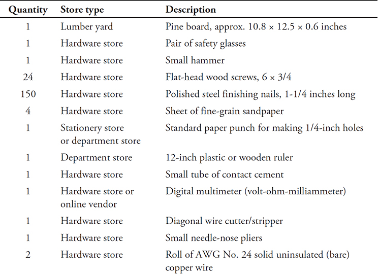

Your breadboard doesn’t have to look fancy or cost much money. I patronized a local lumber yard to get the wood for mine. I found a length of “12-inch by 3/4-inch” pine in their scrap heap. The actual width of a “12-inch” board is about 10.8 inches (27.4 centimeters), and the actual thickness is about 0.6 inch (15 millimeters). The people at the lumber yard didn’t charge me anything for the wood itself, but they demanded a couple of dollars to make a clean cut to produce a rectangular piece of pine measuring 12.5 inches (31.8 centimeters) long.
Using a ruler, divide the breadboard lengthwise at 1-inch (25.4-millimeter) intervals, centered to get 11 evenly spaced marks. Do the same thing going sideways to obtain nine marks at 1-inch (25.4-millimeter) intervals. Using a ball-point or roller-point pen, draw lines parallel to the edges of the board to make a grid pattern. Label the grid lines from A to K and 0 to 9 as shown in Fig. 6-1. That’ll give you 99 intersection points, each of which you can designate with a letter/number pair such as D-3 or G-8.

FIG. 6-1 Breadboard layout for electricity experiments. Solid dots show nail locations. Grid squares measure 1 by 1 inch (25.4 by 25.4 millimeters).
Once you’ve marked the grid lines, gather together a bunch of 1.25-inch (31.8-millimeter) polished steel finishing nails. Place the board on a solid surface that can’t suffer any damage from scratching or scraping. Pound a nail into each intersection point shown by the black dots in Fig. 6-1. Make certain that the nails have “tiny heads” and do not have any coating of paint, plastic, lacquer, or other electrically insulating material. Each nail should go into the board just far enough so that you can’t wiggle it around. I pounded every nail down to a depth of approximately 0.3 inch (8 millimeters), a distance amounting to halfway through the board.
Use some 6 × 32 flat-head wood screws to secure the two miniature lamp holders to the board at the locations shown in Fig. 6-1. Connect the terminals of one lamp holder to breadboard nails A-2 and D-1 with short lengths of thin, solid, bare copper wire. Connect the terminals of the other lamp holder to nails D-2 and G-1. Wrap the wire tightly three or four times around each nail. Snip off any excess wire that remains. Glue the four-cell AA battery holder to the breadboard with contact cement. Allow the cement to harden. That process will need a few hours, so you can take a break for awhile!
When the contact cement has solidified, strip approximately 1 inch (25.4 millimeters) of the insulation from the ends of the cell-holder leads and connect the leads to the nails as shown in Fig. 6-1. Remember that the red lead goes to the positive battery terminal, and the black lead goes to the negative terminal. Use the same wire-wrapping technique that you did for the lamp-holder wires. Place four brand new AA alkaline cells in the holders with the negative terminals against the springs. I recommend that you buy a single package of four cells so that they’re all equally “fresh.” Now you have a 6-V battery, and the breadboard awaits your exploits.
Wire Wrapping
The following breadboard-based experiments employ a construction method called wire wrapping. Each nail forms a terminal to which you can attach component leads or wires. To make a connection, tightly wrap an uninsulated wire or lead around a nail. Make four or five complete wire turns as shown in Fig. 6-2.
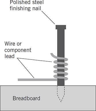
FIG. 6-2 Wire-wrapping technique. If necessary, you can use a diagonal cutter to snip off excess wire.
After you wrap the end of a length of wire, cut off the excess. For small components such as resistors and diodes, wrap the leads around the nails as many times as it takes to use up the entire lead length. That way, you won’t have to cut down the component leads, and you can later unwrap and reuse the components for other experiments. Needle-nose pliers can help you to wrap wires or leads that you can’t wrap with your fingers alone.
When you want to make multiple connections to a single nail, you can wrap one wire or lead over the other, but you shouldn’t have to do that unless you’ve run out of nail space. Each nail should protrude far enough above the board surface so that you won’t get cramped for wrapping space very often.
As you build the circuits that follow, you can tailor the arrangement of parts on the breadboard to suit your needs. I’ve provided schematic and pictorial diagrams to show you how the components interconnect. I recommend that you follow my layout suggestions. That way, you can focus on how the actual appearance of the circuit compares with the schematic, even if you haven’t bothered to build the breadboard and work with the hardware directly.
Small components such as resistors should go between adjacent nails (either straight or diagonally) so you can wrap each lead securely around each nail. If the nails lie too distant from each other, the component leads might not reach far enough to allow decent wrappings. You should secure jumper wires, also known as clip leads, to the nails so that their “jaws” can’t easily work their way loose. I suggest that you clamp the jumpers to the nails sideways so the wires come off horizontally. If you try to put one of these so-called alligator clips down on a nail vertically, it might pop off in the middle of a mission-critical operation!
Kirchhoff’s Current Law
In this experiment, you’ll construct a network that demonstrates one of the most important principles in DC electricity. You’ll need five resistors: two rated at 330 ohms, one rated at 1000 ohms (1 k), and two rated at 1500 ohms (1.5 k). You’ll also need four AA cells. In my opinion, Duracell and Eveready sell the best electrochemical cells and batteries in the United States.
Mount the resistors on the breadboard by connecting them between pairs of terminals as shown in Fig. 6-3. Test each resistor with your multimeter (set to function as an ohmmeter) to verify its ohmic value before you install it. Use a 5-inch (13-centimeter) length of bare copper wire to interconnect the three terminals I-1, J-1, and K-1. Do the same thing with I-3, J-3, and K-3, and also with I-5, J-5, and K-5.

FIG. 6-3 Arrangement of resistors on breadboard for demonstration of Kirchhoff’s current law. All resistance values are in ohms. Solid dots indicate breadboard terminals. Solid lines show interconnections with bare copper wire. Dashed lines indicate jumpers.
Gustav Robert Kirchhoff (1824–1887) did research and formulated theories in a time when people didn’t know much about electrical current. He used common sense to deduce the fundamental properties of DC circuits. Kirchhoff reasoned that the current entering any branch point in a circuit must always equal the current leaving that point. Kirchhoff’s current law holds true no matter how many branches enter a given point, and no matter how many branches leave it.
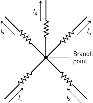
FIG. 6-4 According to Kirchhoff’s current law, the sum of the currents flowing into any branch point always equals the sum of the currents flowing out of that branch point. In this example, I1 + I2 = I3 + I4 + I5.
Connect your four-cell battery to the resistive network and measure the currents in each branch. Meter each test point individually while all the other test points remain shorted with jumpers. The schematic of Figure 6-5 shows the actual values of the resistors in my network (yours will doubtless differ slightly from mine), along with the value I got when I measured I1, the current through the smaller of the two input resistors.
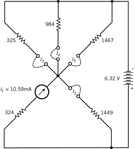
FIG. 6-5 Network for verifying Kirchhoff’s current law. All resistance values are in ohms. The battery voltage, the current I1, and the resistances indicate my measurements. Dashed lines show interconnections with jumpers.
As you measure each current value, make sure that the meter polarity agrees with the battery polarity. The black probe should go to the more negative point, and the red probe should go to the more positive point. That way, you’ll avoid negative current readings that might throw off your calculations. When I tested my four-cell battery to determine its voltage, I got 6.32 V. When I measured I1 through I5, I got the following results, accurate to the nearest hundredth of a milliampere (mA):
I1 = 10.59 mA
I2 = 2.40 mA
I3 = 8.35 mA
I4 = 2.79 mA
I5 = 1.88 mA
Again, make certain that every pair of test points not undergoing current measurement gets shorted together with jumpers. Otherwise, you’ll have an incomplete network, and your current measurements will turn out wrong. After you’ve finished making the measurements, remove all the jumpers to conserve battery energy.
Now you can input your numbers to the Kirchhoff formulas and see how close the sum of the input currents comes to the sum of the output currents. Here are my results for the sum of the currents entering the branch point:
![]()
When I added the currents leaving the branch point, I got
![]()
Kirchhoff’s Voltage Law
In this experiment, you’ll construct a network that demonstrates another important DC circuit rule. You’ll need four resistors: one rated at 220 ohms, one rated at 330 ohms, one rated at 470 ohms, and one rated at 680 ohms. You’ll need four AA cells again, too.
According to Kirchhoff’s voltage law, the sum of the potentials (voltages) across the individual components in a series DC circuit, taking polarity into account, always equals zero. You can also call this rule Kirchhoff’s second law or the principle of voltage conservation.
Ponder the Potentials
Figure 6-6 shows a generic example of Kirchhoff’s voltage law. The battery potential, E, equals the sum of the potentials across the resistors. The polarity across each resistor opposes the polarity of the battery, so that:
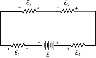
FIG. 6-6 According to Kirchhoff’s voltage law, the sum of the voltages across the resistances in a series DC circuit always equals the battery voltage, but with the opposite polarity. If you disregard polarity, then in this example you’ll get E = E1 + E2 + E3 + E4.
E + E1 + E2 + E3 + E4 = 0
If you measure the potentials across the individual resistors and the battery, one at a time, with a DC voltmeter and disregard the polarity, you’ll find that:
E = E1 + E2 + E3 + E4
Check each of the four resistors with your ohmmeter to verify their values before you install them in the circuit. Mount the resistors in the upper right-hand corner of your breadboard by wrapping the leads around the nails to get the arrangement of Fig. 6-7. Connect the battery to the network with jumpers as indicated, and then measure the voltage across each resistor. Figure 6-8 illustrates the actual values of the resistors in my network (no doubt yours will differ a bit), along with the resistance across which E2 appeared. I measured E = 6.30 V across the battery when I connected it to the resistors.

FIG. 6-7 Suggested arrangement of resistors on breadboard for demonstration of Kirchhoff’s voltage law. All resistance values are in ohms. Solid dots indicate terminals. Dashed lines indicate jumpers.

FIG. 6-8 Network for verifying Kirchhoff’s voltage law. All resistances are in ohms. The battery voltage E, the voltage across the second resistor, and the resistances are the values I measured.
As you measure each voltage E1 through E4, the black meter probe should go to the more negative voltage point and the red probe should go to the more positive point to avoid negative readings that could mess up your calculations. When I measured the voltages across the individual resistors, I got

When you finish making your measurements, remove one of the jumpers to take the stress off the battery.
After you’ve double-checked and written down your voltage measurements, input the numbers to the modified Kirchhoff formula:
E = E1 + E2 + E3 + E4
and see how closely it works out. I got the following results:
E = 6.30 V
and:
![]()
That’s an error of only 0.01 V out of a total potential of 6.30 V, amounting to less than two-tenths of one percent.
A Resistive Voltage Divider
You can use the components from the previous experiment to get several different voltages from a single battery. Keep the resistors on the breadboard in the same arrangement as you had them in the experiment for Kirchhoff’s voltage law.
When you connect two or more resistors in series with a DC power source, those resistors produce various voltage ratios. You can tailor these ratios using specific resistances that “fix” the intermediate voltages. The circuit works best when your network resistors have values much smaller than the resistance of any external load that you place across the combination.
Figure 6-9 illustrates the principle of a resistive voltage divider. The individual resistances are R1, R2, R3, …, and Rn. The total resistance R equals their sum:
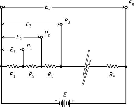
FIG. 6-9 A voltage divider takes advantage of the potential differences across individual resistors connected in series with a DC power source. Note the use of italics for voltages, test points, and resistances.
R = R1 + R2 + R3 + … + Rn
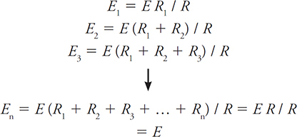
At points P1, P2, P3, …, and Pn, let’s call the voltages relative to the negative battery terminal E1, E2, E3, …, and En, respectively. The last (and highest) voltage, En, equals the battery voltage, E. The voltages at the various points increase according to the sum total of the resistances up to each point, in proportion to the total resistance, multiplied by the battery voltage. In theory, the following equations hold true:
During this experiment, I measured E = 6.30 V across the battery when it operated under a load of all the series-connected resistors in Figs. 6-10A and B. Then I connected the voltmeter across the series combination of the first two resistors only. (Figure 6-10A shows the rated values of the resistors while Fig. 6-10B shows the values I read from my ohmmeter.) I measured the resistances as follows:
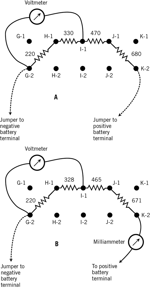
FIG. 6-10 At A, arrangement for measuring voltages in a resistive divider. Here, the voltmeter is connected to measure the potential difference E2 across the series combination of the first and second resistors. All resistances are in ohms. Solid dots indicate terminals. Dashed lines indicate jumpers. At B, arrangement for measuring current through the network. At A, the resistances are the rated values. At B, the resistances are my measured values.
R1 = 220 ohms
R2 = 328 ohms
R3 = 465 ohms
R4 = 671 ohms
Set your meter to measure current in milliamperes (mA). Connect the battery to the resistive network through the meter as shown in Fig. 6-10B, and measure the current. According to strict theory, I expected the milliammeter to indicate a value equal to the battery voltage divided by the sum of my measured resistances:

When I measured the current, I got 3.73 mA, a value only a hundredth of a milliampere (0.01 mA) different from the theoretical value!
Now measure the intermediate voltages E1 through E4 with your meter set for a moderate DC voltage range. The black meter probe should go directly to the negative battery terminal and stay there. The red meter probe should go to each positive voltage point in turn. First measure the voltage E1 that appears across R1 only. Then measure, in order, the voltages as illustrated in the schematic of Fig. 6-9 (assuming n = 4):
• The potential E2 across R1 + R2
• The potential E3 across R1 + R2 + R3
• The potential E4 across R1 + R2 + R3 + R4

FIG. 6-11 Circuit for testing the operation of a resistive voltage divider. The battery voltage E, the potential difference E2 across the series combination of the first and second resistors, and the resistances represent my measurements.
Now connect the meter across the combination R1 + R2. Run jumper wires to the ends of a load resistor located elsewhere on the breadboard, as shown in the layout diagram of Fig. 6-12. This arrangement will cause the voltage source E2 to drive some current through the load resistor (which we’ll call RL), in addition to some current that will keep flowing through R1 and R2. Try every resistor in your repertoire in the place of RL. If you obtained all the resistors in the parts list, you’ll have seven tests to do, using resistors rated at values ranging from 220 to 3300 ohms.
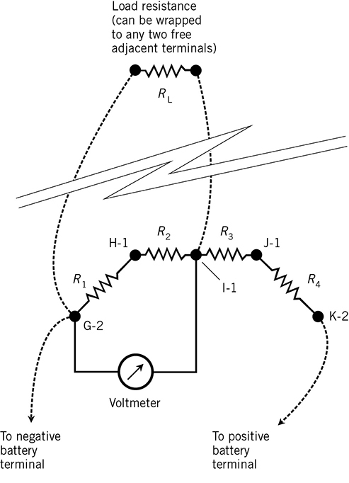
FIG. 6-12 Circuit for testing a resistive voltage divider under load. Dashed lines indicate jumpers. This diagram shows the arrangement for measuring variations in E2 as the load resistance RL is alternately connected and disconnected from the series combination of R1 and R2.
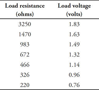
Alternately, connect and disconnect one of the jumper wires between the voltage divider and RL, so you can observe the effect of the extra load on E2. As you’ll see, the additional load affects the behavior of the voltage divider. As RL decreases, so does E2. The effect grows more dramatic as RL decreases, representing a “heavier and heavier load.” Table 6-2 shows the results I got.
TABLE 6-2 Here are the voltages that I measured across various loads in a resistive voltage divider constructed according to Fig. 6-12. My measured network resistances, indicated in the text, were R1 = 220 ohms, R2 = 328 ohms, R3 = 465 ohms, and R4 = 671 ohms. My measured load resistances (left column), which differed a bit from the network resistances (because they involved different physical components!), were the actual values for resistors rated at 3300, 1500, 1000, 680, 470, 330, and 220 ohms, respectively as you read down.
Plot your results as points on a coordinate grid with RL on the horizontal axis and E2 on the vertical axis. Connect the dots to approximate a characteristic curve that shows E2 as a function of RL. Figure 6-13 is the graph I made. I used a reverse logarithmic scale to portray RL so the values would appear spread out. This graph provides a clear picture of what happens as the conductance of the load increases.

FIG. 6-13 My measurements of output voltage vs. load resistance RL in the voltage divider. The dashed line shows the open-circuit (no-load) voltage across the combination of R1 and R2 in series. Open circles show the measured voltages across various loads. The solid curve lets you see how the circuit behaves as RL goes down.
A Diode-Based Voltage Reducer
Rectifier diodes can reduce the output voltage of a DC power source, providing a more predictable way to get specific voltages than a resistive divider can do. Let’s build one! For this experiment, you’ll need two rectifier diodes. Those that I obtained were rated at 1 A and 600 peak inverse volts (PIV), although higher ratings will work too. You’ll also need at least one of each resistor listed in Table 6-1, along with some jumpers.
Figure 6-14 shows the schematic symbol for a rectifier diode. Manufacturers can produce one of these things by joining a piece of P-type semiconductor material to a piece of N-type material, creating a so-called P-N junction. The N-type semiconductor, represented by the short, straight line, forms the cathode. The P-type semiconductor, represented by the arrow, forms the anode. Under most conditions, electrons can move easily from the cathode to the anode (against the arrow), but not from the anode to the cathode (with the arrow). Conventional or theoretical current, which always goes from positive to negative, flows in the direction that the arrow points.

FIG. 6-14 Schematic symbol for a semiconductor diode. The line represents the cathode. The arrow represents the anode.
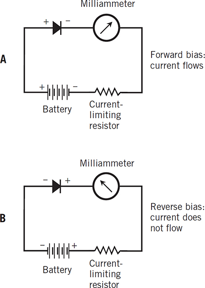
FIG. 6-15 Series connection of a battery, resistor, current meter, and diode. At A, forward bias allows current to flow if the voltage equals or exceeds the forward breakover threshold. At B, reverse bias drives no current through the diode (unless the voltage gets very high).
It takes a certain minimum voltage to drive current through a forward-biased diode. Engineers call this threshold the forward breaker voltage. In most diodes it’s a fraction of a volt, but it varies somewhat depending on how much current you force the diode to carry. If the forward-bias voltage across the P-N junction does not equal or exceed the forward breaker voltage, then the diode won’t conduct. When you forward-bias a diode and connect it in series with a resistor and a battery, the P-N junction voltage goes down to an extent approximately equal to the forward breakover voltage. Unlike the voltage reduction that takes place with resistors, a diode’s voltage-dropping capability stays nearly constant as you vary the external load resistance.
Although current won’t normally flow through a reverse-biased diode, exceptions occur. If the reverse voltage gets high enough (usually much more than the forward breakover value), a diode will conduct because of so-called avalanche effect. Zener diodes, often used to regulate DC power-supply voltage, work according to this principle.
You can set up a voltage reducer with two diodes in series and their polarities in agreement as shown in Fig. 6-16, so that current flows through the load resistor RL if the forward bias voltage is high enough. Figure 6-17 shows an arrangement for mounting the components on your breadboard. Set your meter to indicate DC voltage in a moderate range such as 0 to 20 V. Connect the meter across the load resistance RL, paying attention to the polarity so that you’ll get positive meter readings. Try each one of your resistors in the place of RL. Measure the voltage across RL in every case. You’ll have seven tests to do, with rated resistances ranging from 220 to 3300 ohms.

FIG. 6-16 Schematic showing voltage measurement across the load resistance in a two-diode voltage reducer.

FIG. 6-17 Suggested breadboard layout for measuring voltage across the load resistance RL in a two-diode voltage reducer. Solid dots show breadboard terminals. Dashed lines indicate jumpers. Pay attention to the diode polarities! The cathodes should face toward the negative battery terminal.
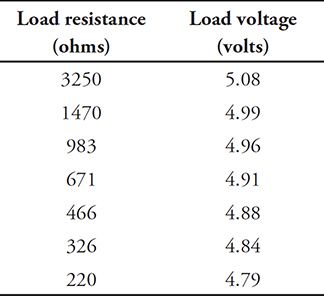
The load resistance RL affects the behavior of a diode-based voltage reducer, but in a different way than it affects the behavior of a resistive voltage divider. As you perform these tests, you’ll see that as the load resistance RL decreases, the potential difference across it goes down, but only a little. The voltage across the load tends to drop more and more slowly as RL decreases. Contrast this behavior with that of the resistive voltage divider, in which the voltage drops off more and more rapidly as RL decreases. Table 6-3 shows the results I got when I measured the voltages across various values of RL with this two-diode arrangement.
TABLE 6-3 Here are the output voltages that I obtained with various loads connected to a diode-based voltage reducer. These are the resistances that I measured. (Yours will of course differ a bit.) The circuit comprised two diodes rated at 1 A and 600 PIV, forward-biased and connected in series with a 6.30-V battery.
Plot your results as points on a coordinate grid with the load resistance RL on the horizontal axis and the voltage across RL on the vertical axis, and then approximate the curve as you did in the previous experiment. I got the graph of Fig. 6-18. As before, I used a reverse logarithmic scale to portray the load resistance. Compare this graph with Fig. 6-13 from the previous experiment.
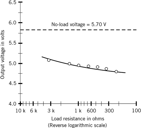
FIG. 6-18 My measurements of output voltage vs. load resistance RL for the two-diode voltage reducer. The dashed line shows the open-circuit (no-load) voltage. Open circles show measured voltages across various loads. The solid curve reveals how the circuit behaves as RL goes down.
Mismatched Lamps in Series
When two dissimilar incandescent lamps operate in series, they receive different voltages and consume different amounts of volt-ampere (VA) power, as this experiment demonstrates. (Remember from your basic electricity courses that in a DC circuit, power in watts equals voltage in volts times current in amperes, hence the term volt-ampere for simple DC power.) You’ll need a 6.3-V lamp, a 7.5-V lamp, a battery of four AA cells, and your multimeter set to measure voltage, as shown in the schematic of Fig. 6-19. You’ll also need some jumpers.

FIG. 6-19 Measurement of voltage E1 across the more negative of two dissimilar lamps in series.
Your breadboard should have two screw-base lamp holders. Position the board so that both holders lie near the top, side by side (Fig. 6-20). Install a 6.3-V lamp in the left-hand socket, and a 7.5-V lamp in the right-hand socket. Connect a short length of bare wire securely between terminals D1 and D2, so the top terminal of the left-hand lamp holder goes to the bottom terminal of the right-hand lamp holder. Then connect jumpers between the free lamp socket terminals and the battery terminals so the lamps operate in series. When you connect the battery to send current through the lamps, they both should glow at partial brilliance.
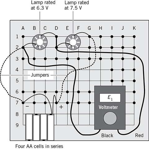
FIG. 6-20 Breadboard layout for the schematic of Fig. 6-19.
Call the lamp closer to the negative battery terminal “lamp N.” That should be the one on the left. Call the lamp closer to the positive battery terminal “lamp P.” That should be the one on the right. Unscrew lamp N. When contact fails, both lamps will go dark. Screw lamp N back in, and then unscrew lamp P. Once again, both lamps will go dark. This demonstrates how a series circuit behaves: A break at any point prevents current from flowing anywhere in the circuit.
Now short out lamp N (the one rated at 6.3 V) with a jumper. It will go dark because it no longer has any voltage across it, while lamp P (rated at 7.5 V) will attain nearly full brilliance. Then disconnect the jumper from lamp N and move the jumper to short out lamp P instead. Lamp P will go dark while lamp N glows at 100 percent of full brilliance. Again, this behavior typifies series circuits. If any component shorts out, all the others consume more power than before.
Set your meter to read DC volts. Connect the jumpers so the lamps are in series and both glow at partial brilliance. Measure the voltage E1 across lamp N as shown in Figs. 6-19 and 6-20. Then measure the voltage E2 across lamp P as shown in the schematic of Fig. 6-21 and the equivalent layout pictorial of Fig. 6-22. When I performed these tests, I got the meter readings:
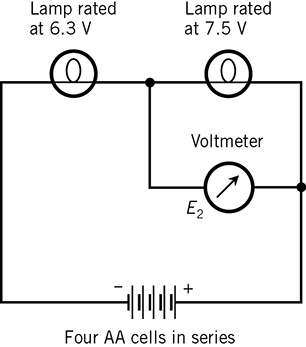
FIG. 6-21 Measurement of voltage across the more positive of two dissimilar lamps in series.
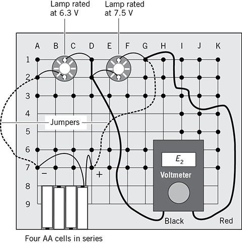
FIG. 6-22 Breadboard layout for the schematic of Fig. 6-21.
E1 = 2.20 V
and:
E2 = 3.64 V
Now determine the voltage E across the series combination of lamps as shown in the schematic of Fig. 6-23 and the layout pictorial of Fig. 6-24. In theory, your meter should display the sum of the lamp voltages, or E = E1 + E2, which equals the battery voltage. When I input the results from my individual lamp tests into this formula, I predicted that I would see

FIG. 6-23 Measurement of voltage E across the combination of two dissimilar lamps in series.
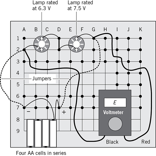
FIG. 6-24 Breadboard layout for the schematic of Fig. 6-23.
E = 2.20 + 3.64
= 5.84 V
My meter showed E = 5.85 V, close to the sum of the voltages across the lamps, but significantly lower than the 6.30 V battery voltage that I got under no-load conditions. Evidently, these bulbs load down the four-cell battery quite a lot. I also entertained the notion that some or all of the AA cells might have grown a little weak during the course of my experiments.

FIG. 6-25 Measurement of current I drawn by the combination of two dissimilar lamps in series.
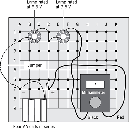
FIG. 6-26 Breadboard layout for the schematic of Fig. 6-25.
Now that you know the voltage across each lamp and the current going through the whole circuit, you can determine VA power numbers for the lamps individually and together. Let PVA1 represent the VA power consumed by lamp N, and use the formula:
PVA1 = E1 I
My results came out as:
![]()
Letting PVA2 represent the VA power consumed by lamp P, the formula is:
PVA2 = E2 I
In this case, I got:
![]()
Now suppose that PVA represents the VA power consumed by both lamps operating together. In that case, theory predicts that:
PVA = E I
When I input my experimental results, I got
![]()
In theory, the VA power consumed by the lamp combination should also work out as the sum of the two VA power quantities taken individually:
PVA = PVA1 + PVA2
Adding my results of PVA1 = 0.306 and PVA2 = 0.506 gave me:
![]()
The error between my two results was a small fraction of one percent, a state of affairs that made me happy indeed!
A Compass-Based Galvanometer
In this experiment, you’ll see how a current-carrying coil affects the behavior of a magnetic compass. The production of a magnetic field by an electric current is called galvanism. You’ll need a camper’s or hiker’s compass calibrated in degrees, 3 feet (1 meter) of enamel-coated magnet wire, a sheet of fine-grain sandpaper, several resistors from your collection, six fresh AA cells, and some jumpers. You’ll need your breadboard equipped with one holder for four AA cells and two holders for single AA cells. You’ll also need a “paper punch” that can put 1/4-inch (6.4-millimeter) holes in thin cardboard.
When you place a compass near a wire that carries DC, the compass doesn’t point exactly toward geomagnetic north. Instead, its needle rotates to the east or west. The rotation extent depends on how close you bring the compass to the wire, and on how much current the wire carries. The rotation direction depends on which way the current flows through the wire and on which side of the compass you place the wire. (The wire should always lie in the same plane as the compass surface.)
When you place a compass on a horizontal surface so the needle points toward N on the scale (geomagnetic azimuth 0°) with zero current flowing in the coil, the needle will point toward geomagnetic north provided no nearby magnetic objects interfere with the geomagnetic field near the compass. When you connect a battery to the coil, the compass needle will move. As you connect higher-voltage batteries to increase the current, the compass needle deflection angle will increase, but it will never rotate more than 90° either way. Reversing the polarity of the applied voltage will reverse the direction of the needle deflection.
Wind 8-1/2 turns of enameled (not bare) copper wire around a magnetic compass so the coil turns lie along the N-S axis of the compass as shown in Fig. 6-27. Use small-gauge, enamel-coated wire of the sort available at most hardware stores. To ensure that you get a mechanically stable coil, glue the compass onto a rectangular sheet of thin cardboard, use the “paper punch” to put holes in the cardboard just above the N and just below the S, and then wind the wire through the holes, passing the wire alternately over and under the compass. Leave roughly 4 inches (10 centimeters) of wire to spare at each end of the coil.

FIG. 6-27 The galvanometer and associated circuitry. The compass must lie flat on a horizontal surface. Place it so the needle points toward N (geomagnetic azimuth 0°) when you disconnect the battery.
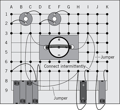
FIG. 6-28 Suggested placement of the galvanometer on the breadboard. The jumper for the positive cell terminal should normally be disconnected. Never connect this jumper to the cell for more than a couple of seconds at a time. In this drawing, geomagnetic north lies off toward the right. Note the two additional single-cell holders in the lower right-hand part of the board.
Use a sheet of fine sandpaper to remove 1 inch (2.54 centimeters) of enamel from each end of the wire. Place the compass onto your breadboard, and wind each sanded-off end of the wire around one of the terminal nails. If the wires are too long, trim them so they’ll fit neatly between the coil and the breadboard terminals after you’ve sanded off the ends. Figure 6-28 shows my layout. This drawing is oriented so the right-hand side of the breadboard points toward geomagnetic north. Align the board so the compass needle points toward N on the scale. Make sure that the coil carries no current.
Use a jumper to connect one end of the coil to the negative terminal of a single AA cell. Connect another jumper to the other end of the coil. Then, for a couple of seconds, touch the “non-coil” end of that jumper to the positive cell terminal. The compass needle should rotate clockwise or counterclockwise by almost 90° so it points either slightly north of geomagnetic east or slightly north of geomagnetic west. Don’t leave the galvanometer connected directly to the cell for more than a couple of seconds at a time, because the coil creates an almost perfect short circuit across the cell.
Take a resistor rated at 680 ohms, another rated at 470 ohms, another rated at 330 ohms, and five more rated at 220 ohms. Use the series combination of four AA cells from the past few experiments. With a jumper, connect the negative battery terminal to one end of the galvanometer coil. Choose two adjacent nails on the board as the location for the resistance to go in series with the galvanometer. Wrap the leads of a 680-ohm resistor around these nails. Using another jumper, connect one end of the resistor to the positive battery terminal. Switch your digital meter to a moderate DC current range. My meter has a setting for 0 to 200 mA. This worked well for me.
Disconnect your digital meter and replace the 680-ohm resistor with one rated at 470 ohms. Repeat the current-vs.-deflection experiment. Do the same with the 330-ohm resistor, and then with the 220-ohm resistor. Keep track of all your digital meter and galvanometer readings in tabular form.

FIG. 6-29 Arrangement for testing the galvanometer. Make sure the compass needle points exactly toward N on the scale under no-current conditions, and deflects toward the east of N when current flows through the coil.
Wrap a second 220-ohm resistor in parallel with the existing one so you get 110 ohms. Repeat the measurements. Add a third 220-ohm resistor to the parallel combination to get approximately 73 ohms, and test the system again. Then add a fourth 220-ohm resistor in parallel, getting about 55 ohms; test again. Then add a fifth 220-ohm resistor to get about 44 ohms, and test yet another time.
Increase the battery voltage by taking advantage of the single-cell holders. Place a fresh AA cell into each holder. Wire one of the new cells in series with the four existing cells to get a five-cell battery, and repeat the experiment with 44 ohms of resistance. Then wire another new cell in series to get a six-cell battery, and once again, do the experiment with 44 ohms of resistance.
After you’ve made all the measurements and written down all the readings from your digital current meter and galvanometer, compile a table showing the number of AA cells in the first (leftmost) column, the rated resistor values in the second column, the current levels in the third column, and the compass needle deflection angles in the fourth (rightmost) column. Table 6-4 shows my results. Yours will doubtless differ somewhat from mine.
TABLE 6-4 Current levels and deflection angles that I obtained with AA cells and resistors in series with a compass-based galvanometer.
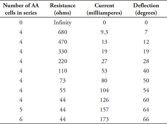
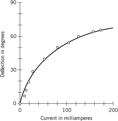
FIG. 6-30 Compass needle deflection vs. coil current for the DC galvanometer. This graph reflects my experimental results, which appear in Table 6-4.
Summary and Conclusion
When you want to design, build, debug, and troubleshoot electronic equipment, you’ll do best if you have a good schematic (or set of schematics) to work with. Pictorial diagrams, including layouts, can help. But when you get in your lab and do the physical work, you’ll never find any substitute for real-world hardware.
If you did all the experiments in this chapter, you almost certainly came up with results a little different from mine. If you had to make major parts substitutions, for example, with the lamps in the last experiment, then some of your results came out a lot different than mine. Whether you performed the experiments or merely followed along in your imagination, you got a chance to see how schematics, pictorials, graphs, and tables can work together. All these tools belong in an engineer’s knowledge base.
Again, please let me make a “shameless plug” for my book Electricity Experiments You Can Do at Home. You’ll get some hands-on lab experience and a bit of theory from that book. You’ll also see some rather strange phenomena! If you want a more exhaustive presentation of electricity and electronics along with plenty of schematics and enough mathematics to keep a true nerd from getting bored, I recommend the latest edition of my book Teach Yourself Electricity and Electronics. Both books are published by McGraw-Hill, and you can find them at major online retailers. You might even come across them at an old-style “bricks and mortar” book store or your local public or school library!