
CHAPTER 5
IDA Pro
In this chapter, we cover the following topics:
• Introduction to IDA Pro for reverse engineering
• Navigating IDA Pro
• IDA Pro features and functionality
• Debugging with IDA Pro
The disassembler and debugger known as Interactive Disassembler (IDA) Pro is a feature-rich, extensible, reverse engineering application owned and maintained by the company Hex-Rays in Belgium. It is a commercial product with alternative versions available such as IDA Home and IDA Free. The IDA family of disassemblers are actively maintained with a large number of freely available plug-ins and scripts provided by Hex-Rays and the user community. Hex-Rays also offers the Hex-Rays Decompiler, arguably the best decompiler available. Compared to other disassemblers, it is the most mature, supporting the largest number of processor architectures and features.
Introduction to IDA Pro for Reverse Engineering
With the large number of free and alternative disassemblers available, why choose IDA Pro? Free alternative disassemblers include Ghidra (covered in Chapter 4), radare2, and some others. Commercial alternatives include Binary Ninja and Hopper. Each of these alternatives is a great disassembler; however, IDA is highly respected, supporting the most processor architectures, and with the greatest number of plug-ins, scripts, and other extensions. It is widely used by the security research community and offers countless features to aid in the analysis of binaries. Also, free versions of IDA Pro are available, with the most recent being IDA 7.0; however, they tend to be limited in their functionality. We will be using IDA Pro and associated plug-ins in Chapter 18 to perform Microsoft patch analysis to locate code changes that could be indicative of a patched vulnerability. The timely weaponization of a patched vulnerability is a powerful technique used during offensive security engagements.
What Is Disassembly?
First, let’s look at the act of disassembling machine code. This is covered in different ways elsewhere in the book, but it is important to ensure you understand the fundamental purpose of a disassembler in relation to this chapter. For this example, we are using the compiled version of the myAtoi program provided to you in your ~/GHHv6/ch05 folder, having previously cloned the Gray Hat Hacking 6th Edition Git repository. Use the objdump tool installed onto Kali Linux with the following options to disassemble the first eight lines of the main function of the myAtoi program. The -j flag allows you to specify the section; in this case, we are choosing the .text or “code” segment. The -d flag is the option for disassemble. We are grepping for the string “<main>:” and printing eight lines after with the -A8 flag.
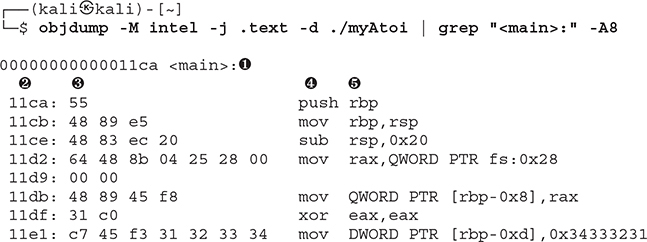
In the first line of output at ![]() , we can see that the main function starts at the relative virtual address (RVA) offset of 0x00000000000011ca from within the overall binary image. The first line of disassembled output in main starts with the offset of 11ca as seen at
, we can see that the main function starts at the relative virtual address (RVA) offset of 0x00000000000011ca from within the overall binary image. The first line of disassembled output in main starts with the offset of 11ca as seen at ![]() , followed by the machine language opcode 55, seen at
, followed by the machine language opcode 55, seen at ![]() . To the right of the opcode at
. To the right of the opcode at ![]() is the corresponding disassembled instruction or mnemonic push, followed by the operand rbp at
is the corresponding disassembled instruction or mnemonic push, followed by the operand rbp at ![]() . This instruction would result in the address or value stored in the rbp register being pushed onto the stack. The successive lines of output each provide the same information, taking the opcodes and displaying the corresponding disassembly. This is an x86-64 bit Executable and Linking Format (ELF) binary. Had this program been compiled for a different processor, such as ARM, the opcodes and disassembled instructions would be different, as each processor architecture has its own instruction set.
. This instruction would result in the address or value stored in the rbp register being pushed onto the stack. The successive lines of output each provide the same information, taking the opcodes and displaying the corresponding disassembly. This is an x86-64 bit Executable and Linking Format (ELF) binary. Had this program been compiled for a different processor, such as ARM, the opcodes and disassembled instructions would be different, as each processor architecture has its own instruction set.
The two primary methods of disassembly are linear sweep and recursive descent (also known as recursive traversal). The objdump tool is an example of a linear sweep disassembler, which starts at the beginning of the code segment, or specified start address, disassembling each opcode in succession. Some architectures have a variable-length instruction set, such as x86-64, and other architectures have set size requirements, such as MIPS, where each instruction is 4-bytes wide. IDA is an example of a recursive descent disassembler, where machine code is disassembled linearly until an instruction is reached that is capable of modifying the control flow, such as a conditional jump or branch. An example of a conditional jump is the instruction jz, which stands for jump if zero. This instruction checks the zero flag (zf) in the FLAGS register to see if it is set. If the flag is set, then the jump is taken. If the flag is not set, then the program counter moves on to the next sequential address, where execution continues.
To add context, the following image shows an arbitrary example inside IDA Pro of a conditional jump after control is returned from a memory allocation function:
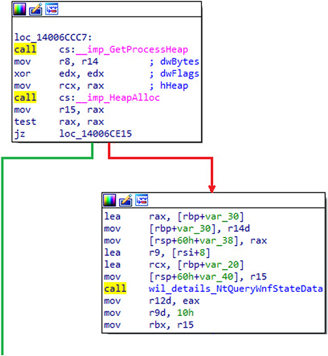
This graphical view inside of IDA Pro is in recursive descent display format.
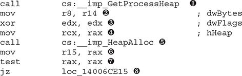
First, the function GetProcessHeap is called ![]() . As the name suggests, this function call returns the base address or handle of the default process heap. The address of the heap is returned to the caller via the RAX register. The arguments for a call to HeapAlloc are now being set up with the first argument being the size, copied from r14 to r8, at
. As the name suggests, this function call returns the base address or handle of the default process heap. The address of the heap is returned to the caller via the RAX register. The arguments for a call to HeapAlloc are now being set up with the first argument being the size, copied from r14 to r8, at ![]() , using the mov instruction. The dwFlags argument is set to a 0 via the xor edx, edx instruction, at
, using the mov instruction. The dwFlags argument is set to a 0 via the xor edx, edx instruction, at ![]() , indicating no new options for the allocation request. The address of the heap is copied from rax into rcx at
, indicating no new options for the allocation request. The address of the heap is copied from rax into rcx at ![]() . Now that the arguments are set up for the HeapAlloc function, the call instruction is executed at
. Now that the arguments are set up for the HeapAlloc function, the call instruction is executed at ![]() . The expected return from the call to HeapAlloc is a pointer to the allocated chunk of memory. The value stored in rax is then copied to r15 at
. The expected return from the call to HeapAlloc is a pointer to the allocated chunk of memory. The value stored in rax is then copied to r15 at ![]() . Next, the test rax, rax instruction is executed at
. Next, the test rax, rax instruction is executed at ![]() . The test instruction performs a bitwise and operation. In this case, we are testing the rax register against itself. The purpose of the test instruction in this example is to check to see if the return value from the call to HeapAlloc is a 0, which would indicate a failure. If rax holds a 0 and we and the register against itself, the zero flag (zf) is set. If the HEAP_GENERATE_EXCEPTIONS option is set via dwFlags during the call to HeapAlloc, exception codes are returned instead of a 0.1 The final instruction in this block is the jump if zero (jz) instruction, at
. The test instruction performs a bitwise and operation. In this case, we are testing the rax register against itself. The purpose of the test instruction in this example is to check to see if the return value from the call to HeapAlloc is a 0, which would indicate a failure. If rax holds a 0 and we and the register against itself, the zero flag (zf) is set. If the HEAP_GENERATE_EXCEPTIONS option is set via dwFlags during the call to HeapAlloc, exception codes are returned instead of a 0.1 The final instruction in this block is the jump if zero (jz) instruction, at ![]() . If the zf is set, meaning that the HeapAlloc call failed, we take the jump; otherwise, we advance linearly to the next sequential address and continue code execution.
. If the zf is set, meaning that the HeapAlloc call failed, we take the jump; otherwise, we advance linearly to the next sequential address and continue code execution.
Navigating IDA Pro
It is important to understand how to properly work with and navigate IDA Pro, as there are many default tabs and windows. Let’s start with an example of loading a basic binary into IDA Pro as an input file. When first loading the myAtoi program into IDA Pro, we are prompted with the following window:
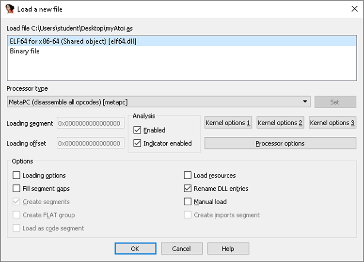
IDA Pro has parsed through the metadata of the object file and determined that it is a 64-bit ELF binary. IDA performs a large amount of initial analysis, such as the tracing of execution flow, the passing of Fast Library Identification and Recognition Technology (FLIRT) signatures, stack pointer tracing, symbol table analysis and function naming, inserting type data when available, and the assignment of location names. After you click OK, IDA Pro performs its auto-analysis. For large input files, the analysis can take some time to complete. Closing all the windows and hiding the Navigator toolbar speeds up the analysis. Once it is completed, clicking Windows from the menu options and choosing Reset Desktop restores the layout to the default setting. Once IDA Pro has finished its auto-analysis of the myAtoi program, we get the result shown in Figure 5-1.
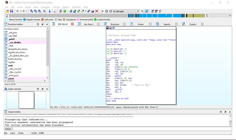
Figure 5-1 IDA Pro default layout

NOTE A lot of features and items are referenced in Figure 5-1. Be sure to refer back to this image as we work our way through the different sections, features, and options.
The Navigator toolbar in Figure 5-2 provides an overview of the entire input file, broken up by the various sections. Each color-coded area within the toolbar is clickable for easy access to that location. In our example with the myAtoi program, a large portion of the overall image is identified as regular functions. This indicates internal functions and executable code compiled into the binary, as opposed to external symbols, which are dynamic dependencies, and library functions, which would indicate statically compiled library code. The Functions window, shown in Figure 5-3, is a list of names for all internal functions and dynamic dependencies.
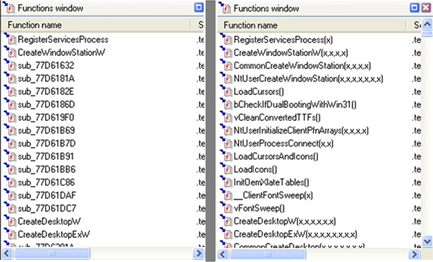
Double-clicking an entry causes that function to display in the main graph view window. The G hotkey also allows you to jump directly to an address. If a symbol table is available to IDA Pro, all functions are named accordingly. If symbol information is not available for a given function, they are given the sub prefix, followed by the Relative Virtual Address (RVA) offset, such as sub_1020. The following is an example of when a symbol table is not available versus when it is available:
![]()
Figure 5-2 IDA Pro Navigation toolbar
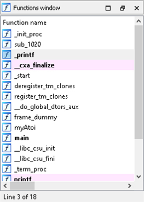
Figure 5-3 IDA Pro Functions window
Below the Functions window is the Graph Overview window. Refer to Figure 5-1 to see this window. It is simply an interactive window representing the entire function currently being analyzed.
The Output window at the bottom of the default IDA Pro layout is shown in Figure 5-4, along with the interactive Python or IDC bar. The Output window is where messages are displayed, as well as the results of entered commands via IDA Python or IDC. IDA Python and IDC are discussed in Chapter 13. In our example, the last message displayed is, “The initial autoanalysis has been finished.”

Figure 5-4 IDA Pro Output window
The main window in the center of IDA Pro’s default layout is titled IDA View-A in our example and is shown in Figure 5-5. This is the graph view, which displays functions and the blocks within those functions in a recursive descent style. Pressing the spacebar within this window switches the display from graph view to text view, as shown in Figure 5-6. Text view is more of a linear sweep way of looking at the disassembly. Pressing the spacebar again toggles between the two view options. In Figure 5-5, the main function is displayed and there is only a single block of code. The type information is displayed at the top of the function, followed by local variables and the disassembly.
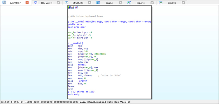
Figure 5-5 IDA Pro graph view
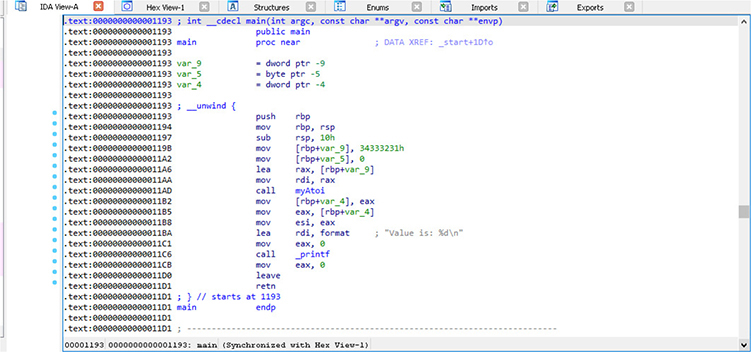
Figure 5-6 IDA Pro text view
Figure 5-7 shows the Imports tab. This window displays all the dynamic dependencies the input file has on library code. The top entry listed is the printf function. The shared object containing this function is required for the program to run and must be mmap’d into the process at runtime. Not shown is the Exports tab. This window displays a list of ordinally accessible exported functions and their associated addresses. Shared objects and Dynamic Link Libraries (DLLs) make use of this section.
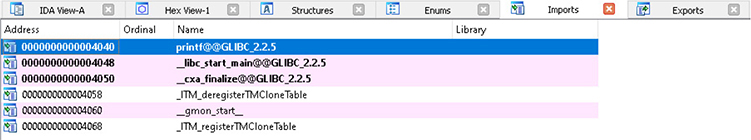
Figure 5-7 IDA Pro Imports tab
IDA Pro Features and Functionality
IDA Pro has a large number of built-in features, tools, and functionality; however, as with many complex applications, there is a learning curve when first getting started. Many of these options are not available in the IDA Free version. We will start with the most basic preference setting, the color scheme, and then go over some of the more useful features. IDA Pro offers different predefined options with the color scheme. To set these options, click the Options menu, followed by Colors. Shown in Figure 5-8 is the IDA Colors drop-down menu and options. You can select between default, darcula, and dark. The dark option applies to IDA Pro in its entirety. The darcula option applies only to the disassembly window. Figure 5-9 shows an example of dark mode.
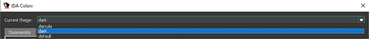
Figure 5-8 IDA Pro color schemes
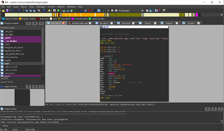
Figure 5-9 IDA Pro dark mode
Cross-References (Xrefs)
It is quite common to want to know from where in a binary there are calls to a function of interest. These are called cross-references, also known as xrefs. Perhaps you want to know from where and when a call to the HeapAlloc function is made. One method is to click the Imports tab, sort the Name column alphabetically, and locate the desired function. When this is located, double-click the name to be taken to the Import Data (.idata) section for the desired function, such as that shown in Figure 5-10. With the function selected within the .idata section, press CTRL-X to bring up the xrefs window. Figure 5-11 has the results in our HeapAlloc example. We can select any of the calls listed to go to that location within the input file.

Figure 5-10 Import data section
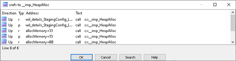
Figure 5-11 Cross-references to HeapAlloc
NOTE There is also an operand cross-reference hotkey called JumpOpXref, which is executed by pressing X. An example use case could be a variable stored in the data segment of a program that is referenced multiple places within the code segment. Pressing X on the variable when highlighted brings up the cross-references to that variable.
Function Calls
Figure 5-12 is an example of a function with quite a few blocks. Functions are often much larger than this example. It is common to want to look at not only all cross-references to a function but also calls from a function. To get this information in one place, select View | Open Subviews | Function Calls. The truncated example in Figure 5-13 shows three calls to the currently analyzed function, as well as quite a few calls from this function.
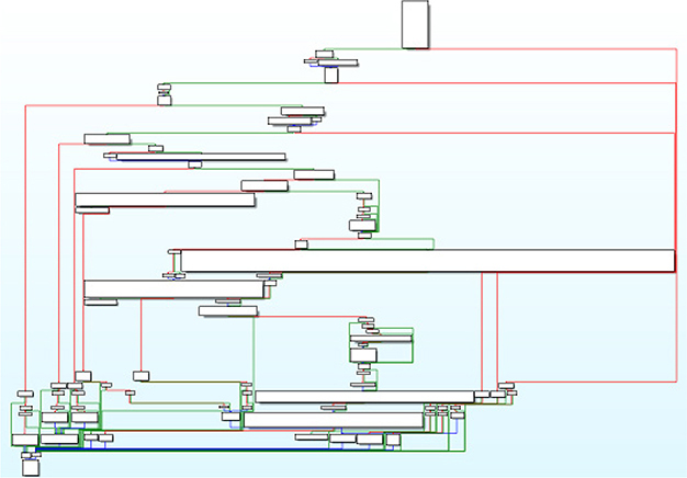
Figure 5-12 Example of a function
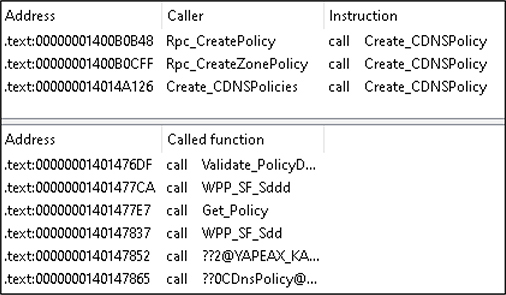
Figure 5-13 Function calls
Proximity Browser
The proximity browser, also known as proximity viewer (PV), feature is useful for tracing paths within a program. Per the Hex-Rays website, “We can use the PV, for example, to visualize the complete callgraph of a program, to see the path between 2 functions or what global variables are referenced from some function.”2 In Figure 5-14 we are using proximity browser to trace the path between the main function and a call to memcpy. The memcpy function has a count argument that specifies the number of bytes to copy. This function is often involved in buffer overruns due to the improper calculation of the count argument, hence why it is used as an example.
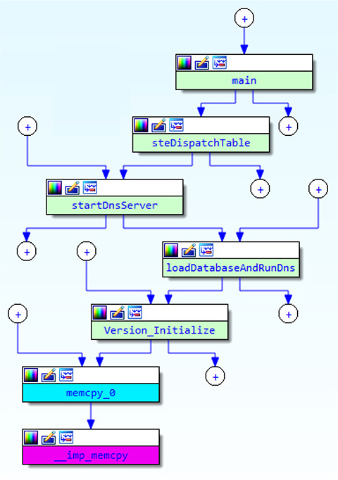
Figure 5-14 Proximity browser
To open the proximity browser, click View | Open Subviews | Proximity Browser. Once there, if anything is displayed by default, you can collapse any child or parent nodes by right-clicking the center node and selecting the appropriate option. If you right-click anywhere in the window that is not a node, you are presented with menu options. The easiest method is to select Add Node by Name and choose the desired function name from the list as either the starting or ending point. You then perform this same operation to select the other point. Finally, you can right-click one of the nodes and select the Find Path option.
Opcodes and Addressing
You may have noticed in the main graph view of IDA that opcodes and addressing are not displayed by default. This information is considered distracting by some analysts and may take up unnecessary screen space, especially in 64-bit programs. Adding this information into the display is very simple and is performed by clicking Options | General. Figure 5-15 shows a screenshot of this menu on the Disassembly tab, where we checked the Line Prefixes (Graph) option while in graph view and set the Number of Opcode Bytes (Graph) field to 10. In Figure 5-16, you can see this information included in the display. You can press CTRL-Z to undo these changes.
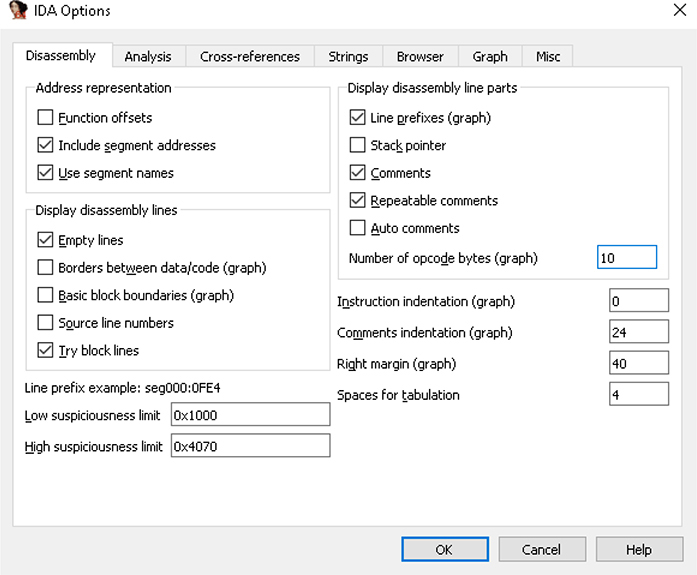
Figure 5-15 General Options menu
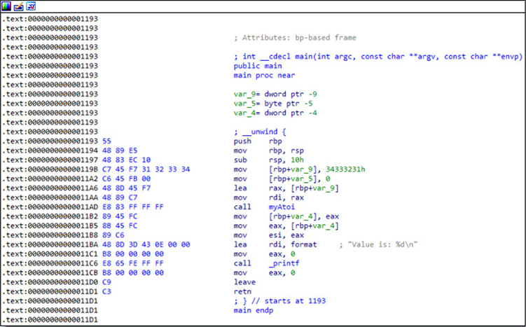
Figure 5-16 Opcodes and address prefixes
Shortcuts
There are a lot of default shortcuts and hotkeys that are not intuitive, such as pressing W to zoom out and the number 1 to zoom in to a predefined size. The numbers 2 and 3 allow you to zoom in and zoom out in a more controlled manner. How do we know these different options? Click Options | Shortcuts to bring up the window that controls these settings. This is shown in Figure 5-17. Here you will find the default hotkeys, as well as those that have been changed. The defaults may vary between the different versions, such as IDA Pro, IDA Home, and IDA Free.
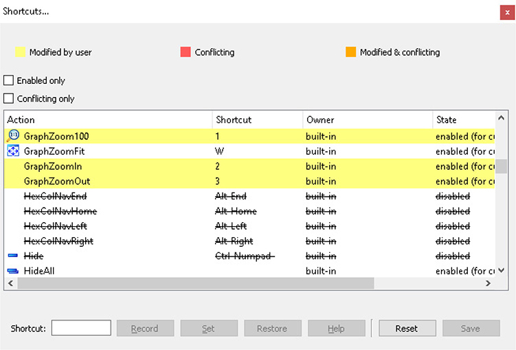
Figure 5-17 Shortcuts menu
Comments
It is common practice to include comments in your code when writing an application. This allows others who look at your code to understand your thought process and get into the same context. As the author, it also makes it easier for you to get back up to speed when opening back up the codebase. This same practice applies to reverse engineering. Looking at disassembly or decompiled pseudocode is a time-consuming practice. IDA adds in some comments based on available type information. There are various types of comments, but two of the most common are regular comments and repeatable comments. To add a regular comment, click the desired line of disassembly and press the colon (:) key. Type in your comment and click OK. An example of a comment is seen in Figure 5-18. Per Hex-Rays, a repeatable comment is “basically equivalent to regular comments with one small distinction: they are repeated in any location which refers to the original comment location. For example, if you add a repeatable comment to a global variable, it will be printed at any place the variable is referenced.”3
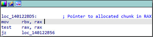
Figure 5-18 Regular comment
Debugging with IDA Pro
IDA Pro includes robust debugging support, both local and remote. Local debugging is supported by the platforms on which IDA Pro is installed, including macOS, Linux, and Windows. Remote debugging is supported on various platforms, including iOS, XNU, BOCHS, Intel PIN, Android, and others. We will focus on a remote debugging example for this section using GDB Server running on a target Kali Linux virtual machine and IDA Pro running on a Windows 10 virtual machine. IDA Pro comes with multiple remote debugging stubs that can be copied to the desired target system where an application is to be debugged.
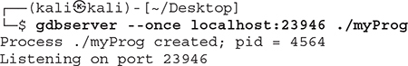
Let’s get right to an example of remote debugging with IDA Pro. For this example, we are using the compiled version of the myProg program provided to you in your ~/GHHv6/ch05 folder, having previously cloned the Gray Hat Hacking 6th Edition Git repository. This is not a lab; however, if you wish to follow along, this program is needed on the system where IDA is installed as well as on the target Kali Linux system. Network connectivity is required between the system running IDA Pro (debugger) and the system running the target program (debuggee), as GDB Server listens on a designated TCP port number and awaits a connection request. The following command starts up GDB Server for the myProg program and tells it to listen on TCP port 23946 to await an incoming connection. The --once option terminates GDB Server after the TCP session closes, as opposed to automatically starting again.
With GDB Server running on the target debuggee system, it is time to load the myProg program into IDA Pro on the debugger system. We allow IDA Pro to perform its auto-analysis and select the Remote GDB Debugger option, as shown in Figure 5-19. We now click Debugger | Process Options from the IDA Pro menu. This brings up the dialog box shown in Figure 5-20. The Application and Input File options are both set to the local folder where the myProg program is located. As an example, if we were debugging a DLL loaded by a target application, the Application and Input File options would be different. For the Hostname option, we have entered the IP address of the target debuggee system. The port number defaults to 23946, so we used this same option on the target system with GDB Server. Once we accept these options, we click the Play button, shown in Figure 5-19. We are then presented with the pop-up that says, “There is already a process being debugged by remote. Do you want to attach to it?” We click Yes, allowing IDA Pro to attach to the remote GDB Server. The debugging attempt is successful, and it pauses execution once attached, as shown in Figure 5-21.
![]()
Figure 5-19 Remote GDB Debugger in IDA
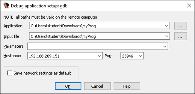
Figure 5-20 IDA debugging options window
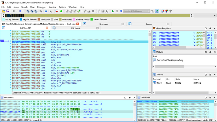
Figure 5-21 IDA Pro remote debugging session
There are several sections within the debugging window. If you are familiar with other debuggers, then the sections should look familiar. The main and larger section, called IDA View-RIP, is the disassembly view. Currently, we can see that the instruction pointer (RIP) is pointing to a memory address holding the instruction mov rdi, rsp. Most of the sections inside the debugging window are scrollable. The section below the disassembly window, called Hex View-1, dumps any desired memory segment in hexadecimal form. To the right of Hex View-1 is the Stack view. This defaults to starting at the stack pointer (RSP) address, dumping the contents of memory for the current thread’s stack. Above the Stack view section are the Threads and Modules sections. Finally, in the top right is the General Registers section. This section shows the general-purpose processor registers as well as additional registers, including the FLAGS register and Segment registers.
Debugger controls are activated through assigned hotkeys, ribbon bar menu icons, or by going through the debugging menu. If we click Play to allow the program to continue execution, it simply terminates, as we have not provided any command-line arguments. When looking at the Imports table within this program, we see there is a call to the deprecated strcpy function, as shown in Figure 5-22. We then use Proximity Browser to trace the path from the main function to strcpy, as shown in Figure 5-23. When looking at the func1 function, we can see the call to strcpy, as well as the buffer size for the destination at 0x40, or 64 bytes. We next set a breakpoint on the call to strcpy, as shown in Figure 5-24, by clicking the address and pressing the F2 breakpoint hotkey.
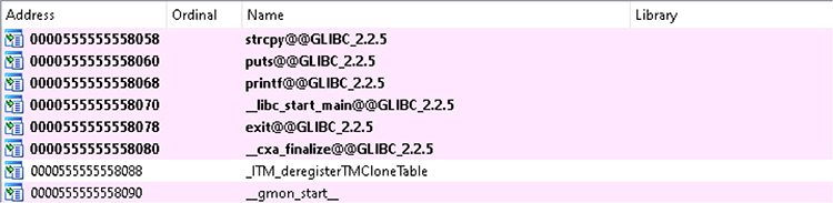
Figure 5-22 Deprecated call to the strcpy function
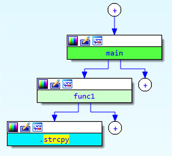
Figure 5-23 Proximity Browser path to strcpy
With the breakpoint set on the strcpy function, and understanding the destination buffer size, let’s pass in 100 bytes as our argument to see if we can get the process to crash. We modify our gdbserver command to include some Python syntax on the end as such:

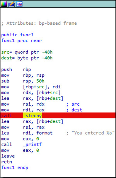
Figure 5-24 Breakpoint set on strcpy
We then click the Play button inside of IDA to initiate the connection to the debuggee. Once attached, we must click the Play button again to continue to our breakpoint on the strcpy function. The result is shown in Figure 5-25. The source argument addressed has been dumped to the Hex View section so that we can see what is going to be copied to the destination buffer on the stack. Pressing the F9 continue execution hotkey in IDA results in an expected crash, as shown in Figure 5-26. Snippets are taken from the debugger that show the warning about a segmentation fault, the resulting General Registers section, and Stack view section.
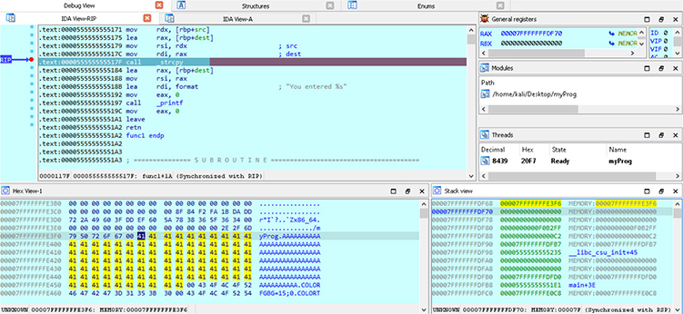
Figure 5-25 Breakpoint on strcpy
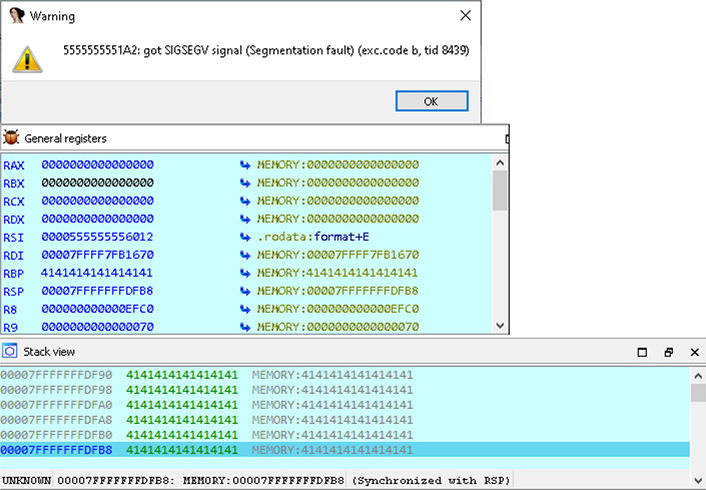
Figure 5-26 Crash caught in IDA Pro Debugger
Having the ability to locally and remotely debug programs using IDA Pro’s graphical front end, along with various debugging stubs, can greatly speed up your analysis.
Summary
This chapter provides you with the basics of getting started in using IDA Pro as a reverse engineering tool. There are far too many features and extensibility options to fit into a single chapter. We looked at getting to know the IDA Pro interface, some of the most commonly used features of IDA, as well as getting up and running with remote debugging. We will be using IDA Pro in later chapters covering Microsoft patch diffing and Windows exploitation. The best way to learn to use IDA Pro is to take a basic C program, like the ones used in this chapter, and start reversing. You can expect to spend a lot of time googling the answers to questions around different assembly instructions and how to do specific things with IDA Pro. You will see your skills quickly improving the more you use the tool and become familiar with reversing with IDA Pro.
For Further Reading
Hex-Rays Blog www.hex-rays.com/blog/
IDA Debugger www.hex-rays.com/products/ida/debugger/
IDA Freeware www.hex-rays.com/products/ida/support/download_freeware/
OpenRCE www.openrce.org/articles/
Reverse Engineering Reddit www.reddit.com/r/ReverseEngineering/
Reverse Engineering Stack Overflow reverseengineering.stackexchange.com
References
1. Microsoft, “Heapalloc function (heapapi.h) – win32 apps” (December 5, 2018), https://docs.microsoft.com/en-us/windows/win32/api/heapapi/nf-heapapi-heapalloc (retrieved March 19, 2021).
2. Koret, J., “New feature in IDA 6.2: The proximity browser” (August 8, 2011), https://www.hex-rays.com/blog/new-feature-in-ida-6-2-the-proximity-browser/ (retrieved March 20, 2021).
3. Skochinsky, I., “Igor’s tip of the week #14: Comments in IDA” (November 6, 2020), https://www.hex-rays.com/blog/igor-tip-of-the-week-14-comments-in-ida/ (retrieved March 20, 2021).